

Abstract

It is important to incorporate the effects of fluid–structure thermal coupling and the boundary conditions when calculating the thermal dynamics and response of progressive cavity pumps. This study develops a fluid–structure thermal coupling model of the progressive cavity pump to improve the accuracy of its measured field of deformation and the temperature field of the stator. A function for the macroscopic motion of a rigid body is written in a typical fluid domain, and the user-defined function (UDF) in FLUENT is used to load the boundary of the rotor to realize its planetary motion. Local remeshing is used to update the moving grid, and the viscoelastic hysteretic heat of the stator is treated as the internal source of heat. One-way decoupling is used based on tire slip theory, and heat flux on the surface of the stator is calculated by the ANSYS Parametric Design Language (APDL). The sequential fluid–structure thermal coupling of the progressive cavity pump is calculated by using the ANSYS workbench. A scheme for optimizing the fit clearance of the stator and rotor is given to improve the volumetric efficiency of the progressive cavity pump and prevent the stator from being stuck owing to a large deformation, and the calculations are verified by experiments on volumetric efficiency. The average deviation in the calculated volumetric efficiency was less than 5% compared with the experimental values. The proposed scheme provides a theoretical basis for the optimal design of the progressive cavity pump for the thermal production of petroleum.
1. Introduction
The progressive cavity pump is a rotary displacement pump installed underground through an interference fit between a rigid rotor and an elastic rubber stator. It is difficult for a progressive cavity pump to function at high speeds and a high temperature of crude oil in a complex environment. Because the stator is made of viscoelastic rubber, it is subjected to elastic deformation under the action of the periodic extrusion of the rotor, hydraulic pressure, and the pressure difference between adjacent chambers. Because the strain in elastic rubber is hysteretic, a large viscous loss occurs due to heat generation during operation, in addition to convective heat transfer between the fluid and the stator, that leads to large deformations in the stator. This reduces the efficiency of the pump and leads to problems such as a burning or stuck pump and the faster aging and degumming of the stator that reduce its service life.1
During the operation of the screw pump, the temperature and stress fields lead to the deformation of the stator, which in turn changes the distribution of the fluid and temperature fields. The temperature field and stress–strain process of the stator involve multiphysical fluid–structure thermal coupling. Three representative methods are typically used to study them:
The physical field is analyzed without considering the effects of coupling.2−6 The elastic deformation of the stator is calculated when it and the rotor are in interference-induced contact, or its stress and strain are calculated when a fixed pressure is applied to the inner cavity of the stator and a pressure difference is set in the adjacent chamber.
The temperature distribution and deformation of the stator are simplified as a process of thermal structure coupling,7−12 ignoring the influence of the pressure and convective heat transfer of the fluid. The temperature field of the stator rubber is regarded as a heat conduction problem with an internal heat source by using the one-way decoupling of its thermodynamics. The thermal–mechanical coupling is decomposed using deformation analysis, loss analysis, and heat conduction analysis to determine the temperature distribution and changes in the profile of the stator.
The deformation of the stator is simplified as a fluid–structure coupling process.13−15 The influence of thermodynamic factors is neglected, the stator is regarded as a deformable body, and multifield coupling software is used to realize unidirectional fluid–structure coupling between the liquid and the stator.
The boundary conditions of the single-field and two-field coupling schemes deviate from the empirical situation. The above methods generally use a two-dimensional (2D) plane model while ignoring the axial heat conduction and deformation of the rotor. This reduces the difficulty of the simulation but also the accuracy of the calculation. By establishing a 3D model and considering the influence of the coupling between various factors, more accurate measurements of the temperature field and characteristics of deformation of the stator can be obtained, which can help optimize the structural design and predict the performance of the progressive cavity pump.
Because the model of the progressive cavity pump is complex and large, indirect coupling, which involves a few calculations and yields a high accuracy, is used here for multiple physical fields. The method involves solving the equations of fluid control, thermodynamics, and solid control according to the sequence of coupling. The data are then transferred at the coupling interface. That is, the fluid domain is solved first and its results (pressure and temperature) are then applied to the structure of the stator as external loads. The rubber stator also requires considering viscoelastic hysteretic heat. We designed a program to calculate the rate of heat generation and loaded this into the stator module as thermal load. Finally, the comprehensive deformation of the stator was calculated. The implementation of the fluid–structure thermal coupling is shown in Figure 1. To verify the reliability of the multifield coupling scheme, two-way coupling was used in this calculation to obtain the volumetric efficiency of the progressive cavity pump. This was compared with the experimental value to verify the reliability of the scheme.
Figure 1.

Calculation of fluid–structure thermal coupling of the progressive cavity pump.
2. Theory of Calculation of Fluid–Structure Thermal Coupling
2.1. Mathematical Expression of Fluid–Structure Coupling
The elastic deformation of the stator under fluid pressure satisfies the dynamic equation of classical mechanics. The contact among the fluid, rotor, and stator can be regarded as elastic contact in a continuous medium and can be solved by using the Lagrangian method. Owing to the nonlinearity of contact, such as that between the stator and the rotor, the geometric nonlinearity of the movement of the rotor, and the material nonlinearity of the stator, the explicit dynamic method is more efficient than the implicit method, especially for different types of nonlinear problems. For non-ideal fluid motion, the governing equations of the Euler method include equations for the conservation of mass, momentum, and energy as well as the state and constitutive equations.
The main governing equations of the fluid domain are as follows:
The equation for the conservation of mass is
| 1 |
where ρ is the density of the fluid, xi represents the three directions of the coordinate system, and ui is the components of velocity along the three directions.
The equation for the conservation of momentum is
| 2 |
where ρ is the density of the fluid, p is the fluid pressure, and ν is the kinematic viscosity.
The equation of energy conservation with temperature T as a variable is
| 3 |
where T is the temperature, k is the heat transfer coefficient, cp is the specific heat capacity, and ST is the viscous dissipation.
For a fluid–solid contact boundary, the mesh of the moving boundary must be generated in each time step owing to the large deformation and displacement of the stator over a short time. To solve this problem, the boundary of the outer contour is blurred, and an additional force term is added to the Navier–Stokes momentum equation to reflect the effect of the boundary.16,17 The equation of constraints on the solid and fluid in the region of coupling is
 |
4 |
The first equation is the Navier–Stokes equation of the fluid, and ΔF is an additional force term that reflects the interaction between the fluid and the structure on the coupling surface. The second equation is the distribution function of the additional force. The third equation is the equation of motion of elastic rubber, A is the energy coefficient, T is the temperature matrix of the stator, and Q(τ) is the heat matrix.
2.2. Mathematical Expression of Coupled Surface Thermal Analysis and Deformation Theory
The rotor performs periodic planetary motion inside the stator, the viscoelastic rubber of which is squeezed and deformed periodically by it to lead to hysteretic heat generation, which can be regarded as an internal heat source. In addition, the fluid in the pump features convective heat transfer with the surface of the stator. Therefore, the temperature field and thermal deformation of the stator are problems of heat conduction under the action of multiple heat sources. For a multidimensional heat conduction problem, it is necessary to combine Fourier’s law with the first law of thermodynamics to deduce the temperature T(x, y, z, t) of the stator. In the rectangular coordinate system, the temperature field of the stator satisfies the following functional expression:
 |
9 |
where ρ is the density of the material, c is its specific heat capacity, kx, ky, and kz are the thermal conductivities of the material in three directions, Q = Q(x,y,z,t) is the density of the heat source within the object, q = q(Γ, t) is the heat flux density on the boundary Γ2, and h is the coefficient of convective heat transfer, Ta = Ta(Γ, t). For the boundary Γ3, φa is the ambient temperature and t is the time.
To obtain the solution for the above heat conduction problem, it is necessary to give reasonable boundary conditions. Viscoelastic hysteretic heat is regarded as the internal heat source, because of which a second boundary condition is used for the boundary of heat generation, that is, the heat flux density of the nodes on the boundary of the stator is given. The heat flux is solved by one-way decoupling analysis. Stress–strain analysis is first carried out and energy loss is then calculated to determine the heat flux.
The stress and strain in a cycle are
| 10 |
| 11 |
where εmax is the maximum strain of the nodes (mm), τmax is their maximum stress (MPa), ω is the deformation frequency (in rad/s), t is the time, and δ is the lag angle (in rad).
The stress and strain are expanded into the superposition of harmonics by the Fourier transform, and the period of calculation is integrated. The loss of energy in one period is obtained as follows:
 |
12 |
where  and
and  are coefficients in the m-order cosine and sine of the ij component of the
strain tensor in the Fourier expansion, respectively, and
are coefficients in the m-order cosine and sine of the ij component of the
strain tensor in the Fourier expansion, respectively, and  and
and  are the coefficients in the m-order cosine and sine in the sinusoidal Fourier expansion of the ij component of equilibrium stress, respectively. The coefficients
in the Fourier expansion can be obtained by using the orthogonality
of the trigonometric function. M is the number of
terms in the Fourier expansion.
are the coefficients in the m-order cosine and sine in the sinusoidal Fourier expansion of the ij component of equilibrium stress, respectively. The coefficients
in the Fourier expansion can be obtained by using the orthogonality
of the trigonometric function. M is the number of
terms in the Fourier expansion.
The heat flux of the unit is
| 13 |
A third kind of boundary condition is adopted for convective heat transfer between the fluid and the stator, that is, given the coefficient of convective heat transfer and the temperature of the fluid on the boundary of the stator, the heat transfer satisfies Newton’s cooling equation:
| 14 |
where h is the convective heat transfer coefficient (W/(M2·K)), obtained by the coupled calculation of flow and heat, Tr is the surface temperature of the cavity of the stator (K), and Tf is the temperature of the liquid in the cavity of the screw pump.
2.3. Thermoelastic Deformation Theory
Because there is a temperature difference in the stator, additional stress and strain are generated in it. Therefore, thermal expansion should be added to the elasticity equation. The physical equation of thermoelasticity can be written as
 |
15 |
| 18 |
where εxx, εyy, and εzz refer to the normal strain, σxx, σyy, and σzz refer to the normal stress, E is the elastic modulus, αT is the coefficient of thermal expansion of the elastomer, μ is the Lame coefficient of elasticity, τxy, τyz, and τzx refer to the shear stress, γxy, γyz, and γzx refer to the shear strain, and G is the shear modulus of elasticity.
Because the profile of the stator remains unchanged along the axial direction, temperature deformation in its cross section is taken as the research object to facilitate the expression of the above problems. The above formula can then be simplified as
 |
19 |
The geometric equations of normal strain and shear strain can be expressed as
 |
22 |
where u and v are the components of displacement in the x and y directions, respectively.
The coupled differential equation of temperature displacement in the stator plane can be derived as
 |
25 |
The expansion-induced deformation of the stator can be obtained by substituting its calculated temperature field into the above formulae.
3. Fluid–Structure Thermal Coupling Model
3.1. Model of the Fluid Domain
The GLB120-27 progressive cavity pump was used as an example to examine multifield coupling. The parameters were as follows: the outer diameter of the stator was 89 mm, that of the stator rubber was 77 mm, the diameter of the rotor was 38 mm, eccentricity was 5 mm, the stator lead was 160 mm, rotor lead was 80 mm, and the speed of the rotor was 150 r/min. There are 27 cavities in the GLB120-27 screw pump, because of which a large amount of calculation was needed for modeling. Because the screw pump had a circulation structure, overall modeling was unnecessary. Only one lead of the screw pump was built as the unit of calculation, and pressures and temperatures of different magnitudes were applied at the boundaries of the inlet and outlet of the model to simulate the working conditions of the upper, middle, and lower segments of the screw pump. To ensure the continuity of the calculation in the fluid domain, the clearance between the stator and the rotor was set to 0.3 mm. The model of the lead channel of the progressive cavity pump is shown in Figure 2.
Figure 2.

Model of the stator, rotor, and flow channel.
To simulate the complex planetary motion of the rotor in the stator, a dynamic mesh model was used to simulate the change in the shape of the fluid domain over time.18 The shape of the channel was complex, and the mixed mesh dominated by hexahedral mesh was selected as the initial mesh (see Figure 3). The grid independence check is shown in Figure 4. When the number of grids is greater than 85 W, the flow rate basically does not change with the number of grids. Therefore, the number of grids used in the calculation is 906,499. The outer surface of the channel was set as the coupling surface and the wall was assumed to be stationary. We wrote the function of the motion of a rigid body (see the procedure below) and applied a user-defined function (UDF) to load on the boundary of the rotor to realize the planetary motion of its moving boundary. The dynamic mesh was activated in the FLUENT interface. The local remeshing method of update was used, which can redivide the mesh according to its rate of distortion and size. The other boundary conditions and settings of the solver are shown in Table 1.
Figure 3.

Flow channel grid of the progressive cavity pump.
Figure 4.
Grid quantity independence check.
Table 1. Boundary Conditions and Solver Settings.
| set condition | definition of boundary condition/initial condition |
|---|---|
| inlet | pressure inlet (p = 3.0 MPa) |
| outlet | pressure outlet (p = 4.0 MPa) |
| coupled (wall) | outer surface of channel |
| flux algorithm | second order upwind |
| solution strategy | SIMPLE |
| turbulence model | realizable K-ε |
| turbulence intensity | 0.01 |
| turbulent viscosity ratio | 10 |
| initial velocity scale of turbulence | 1 m/s |
We called the DEFINE_CG_MOTION (name, dt, vel, omega, time, dtime) macro in FLUENT. It assigns vel and omega to the linear velocity and angular velocity of the center of mass of the rotor, respectively. FLUENT automatically calculated the next position of the rotor. In this program, ω represents the speed, E is the eccentricity, N is the number of threads, eccentric is the UDF file name, and (0, 1, 2) represents the positive direction of (x, y, z) axis.
The program for the UDF in C is as follows:
3.2. Model of the Solid Domain
The stator of the progressive cavity pump was the main research object, the model data are shown in Section 3.1, and the interference was 0.3 mm. The purpose of the coupling calculation was to determine the temperature field and comprehensive field of deformation of the stator. The structures of the stator and rotor are shown in Figure 2.
To ensure the efficiency of calculation, the SOLID185 and SOLID45 elements were used to simulate the stator and rotor, respectively. The number of stator grid elements is 585,025, as shown in Figure 5. To simulate the interference-induced contact between them, CONTA174 and TARG170 were used to simulate the surfaces of the stator and rotor, respectively. Owing to their complex structures, a mixed mesh dominated by hexahedral mesh was used for this calculation. To ensure accuracy, the grid sizes of the stator and rotor were set to 2 mm.
Figure 5.

Stator grid of the progressive cavity pump.
Before the finite element calculation, the parameters of the material and boundary conditions of the stator were set as below.
3.2.1. Conventional Materials and Boundary Conditions of the Stator
-
(1)
The stator was made of butadiene acrylonitrile rubber (NBR). The Mooney–Rivlin material model was used to simulate the stator. The material coefficients were as follows: C10 = 2.00/MPa and C01 = 0.43/MPa. The temperature of the downhole reservoir was 50 °C, the speed of the rotor was 150 r/min, the friction coefficient was 0.1, and the loss factor was 0.2. The other material parameters are shown in Table 2.
-
(2)
In the finite element analysis of stator dynamics, forced displacement and a self-rotation angle were applied to the center of the rotor helix to simulate the planetary motion of the rotor. The forced displacement is
| 28 |
| 29 |
where ω is the angular rotational velocity of the rotor.
Table 2. Performance-Related Parameters of the Rubber Materials.
| kl (W·m–1·K–1) | αl (10–5) | cl (J·kg–1·K–1) | ρl (kg·m–3) | El (MPa) | Poisson’s ratio |
|---|---|---|---|---|---|
| 0.1465 | 1 | 840 | 1200 | 11.48 | 0.499 |
The rotational angle of the rotor is
| 30 |
3.2.2. Boundary Conditions of the Coupling Region
-
(1)
The fluid–solid contact surface, i.e., the inner surface of the stator, was defined as the coupling surface. The temperature of the fluid and the pressure of the coupling surface obtained in the calculations were loaded on the corresponding nodes of the surface of the stator as boundary conditions when calculating the thermal–mechanical coupling of the fluid.
-
(2)
The rate of hysteretic heat generation of viscoelastic rubber, calculated by the above one-way decoupling analysis, was applied to the model to calculate the temperature field of the stator as thermal load. The calculations of the stress–strain and the rate of heat generation of viscoelastic rubber were carried out by using the APDL.
4. Results and Discussion
4.1. Elastic Deformation and Analysis of Fluid–Structure Coupling
According to the laws of distributions of fluid pressure and temperature in the progressive cavity pump,2,10,19,20 pressures of 3.0 and 4.0 MPa, 9.5 and 10.5 MPa, and 15.5 and 16.5 MPa were applied to the inlet and outlet of the fluid domain, respectively, and their temperatures in these segments were set to 50 and 50.4 °C, 51.2 and 52 °C, and 53.6 and 54 °C to simulate the pressure and temperature distributions of the upper, middle, and lower segments of the progressive cavity pump. The temperature-induced expansion caused by convective heat transfer of the fluid is discussed in the next section. This section discusses elastic deformation due to pressure from the fluid.
The fluid–structure coupling analysis and steps of calculation of the screw pump are as follows:21 (1) The fluid domain was calculated by using FLUENT, and the pressure field obtained was input to the structure calculation module as pressure load. (2) A static analysis of the structure was carried out, and the field of elastic deformation generated by the hydraulic pressure was calculated.
Figure 6 shows the results of calculation of fluid pressure at the lower segment of the progressive cavity pump. To clearly see the changes in the pressure of the fluid in the chamber, we chose nine cross sections evenly at an interval of 45° in a lead.
Figure 6.

Pressure distribution of each cross section of the progressive cavity pump at the lower segment.
Figure 6 shows that the chamber pressure gradually increased linearly from the inlet to the outlet. The pressure was not equal in the same cross section, and a pronounced pressure difference was noted on both sides of the meshing line of the stator and rotor. One side of the direction of motion was significantly greater than the other side. Therefore, the application of uniform pressure in the calculation of the pressure-induced deformation of the stator in past work4,6,8,14 is inconsistent with empirical observations.
The pressure calculated in the fluid domain was applied to the surface of the stator as a load to calculate its elastic deformation, as shown in Figure 7. The elastic deformation caused by hydraulic pressure from the inlet to the outlet gradually increased, and the maximum deformation appeared at the outlet. The diagram of cross-sectional deformation shows that deformation at the point of contact with the rotor was the largest, but under the same hydraulic pressure, the maximum elastic deformation in the stator occurred on the inner surface of its thickest wall and gradually decreased on both sides. Due to the differences in pressure on both sides of the meshing surface of the stator and rotor, the deformation in a cross section was also different. Figure 7 also shows the law of contour deformation of the stator at cross sections of ϕ = 90° and 270° along one lead. By taking point A at the thickest part of the stator as the starting point, we rotated it counterclockwise by a full circle to obtain the law of deformation of the contour of its inner cavity. Figure 4 shows that deformation was the largest in the thickest part of the stator and the smallest in its thinnest part. The deformation in the high-pressure chamber was significantly greater than that in the low-pressure chamber.
Figure 7.

Elastic deformation of the lower segment of the stator under hydraulic pressure (90° on the left and 270° on the right).
The laws of deformation of the middle and upper segments were obtained by changing the inlet and outlet pressures of the flow channel. The laws of deformation of the upper, middle, and lower segments were the same, but their deformation values were different. Figure 8 shows a diagram of their deformations at ϕ = 90° and ϕ = 270°. The maximum normal deformation in the stator increased with the hydraulic pressure from the lower to upper segment, and the difference between the maximum and minimum deformations of the inner cavity increased with the hydraulic pressure. The maximum deformation and difference in deformation in the upper segment of the progressive cavity pump, namely, the outlet, were the largest. The increase in this difference is unfavorable for preventing the leakage of the stator. Leakage may occur prematurely in places with large normal deformations, while those with small normal deformations were well sealed.
Figure 8.
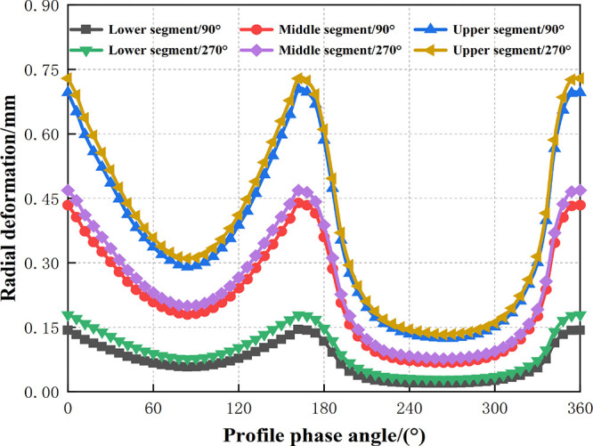
Laws of deformation of the upper, middle, and lower segments of the stator at ϕ = 90° and ϕ = 270°.
4.2. Deformation Field of Thermal Structure Coupling under the Action of Multiple Heat Sources
The steps of implementation of the calculations for thermal structure coupling are as follows: (1) Calculate the field of liquid temperature in FLUENT. (2) Input the calculated temperature field to the thermal analysis module. Calculate the rate of hysteretic heat generation of the viscoelastic rubber from Section 2.2, and apply it to the model of the temperature field of the stator as thermal load. (3) Calculate the temperature field of the stator. (4) Input the results of the structural temperature field to the module for static analysis to calculate the comprehensive field of deformation of the stator.
4.2.1. Thermal Deformation Caused by Fluid Convective Heat Transfer
We set the initial temperature of the stator to 20 °C and loaded the fluid temperature calculated from the previous flow field onto its surface to calculate the thermal deformation caused by convective heat transfer in the stator. The setting of the boundary conditions for thermal deformation owing to convective heat transfer is shown in Figure 9.
Figure 9.

Boundary conditions for convective heat transfer.
The thermal deformation caused by convective heat transfer in the lower segment is shown in Figure 10. The maximum temperature and deformation of the middle and upper segments are shown in Table 3. Figure 10 shows that the maximum thermal deformation caused by fluid convection-induced heat transfer occurred in the thickest part of the cavity of the stator and gradually decreased along both sides. The law was the same as that for deformations due to liquid pressure. The difference was that convective heat transfer caused expansion-induced deformation in the direction opposite to that of pressure-induced deformation. The maximum deformation in the lower segment of the stator from 20 to 50 °C was 0.016 mm, and that caused by a unit rise in temperature was 0.5 × 10⁻³ mm. A comparison with previously obtained pressure deformation values shows that the deformation in the stator caused by convective heat transfer of the fluid alone was far smaller than the compression due to fluid pressure. As the rise in the temperature of the fluid from the inlet to the outlet was not large in case a pure liquid was used, Table 3 shows that the differences among the maximum deformations in the lower, middle, and upper segments were small.
Figure 10.

Thermal deformation caused by convective heat transfer in the lower segment.
Table 3. Maximum Temperature and Deformation due to Convective Heat.
| position | maximum temperature/°C | maximum displacement/(10–2 mm) |
|---|---|---|
| lower segment | 50.383 | 1.649 |
| middle segment | 51.982 | 1.715 |
| upper segment | 53.980 | 1.799 |
4.2.2. Thermal Deformation Caused by Hysteretic Heat of Viscoelastic Rubber
The rotor moved in a periodic planetary manner in the stator, and the viscoelastic rubber was periodically extruded and deformed by it. Owing to different loads, and because rubber is a poor conductor of heat, this periodic extrusion produced an uneven rise in temperature in the stator that led to hysteretic heat. The viscoelastic hysteretic heat of the rubber stator can be regarded as an internal heat source, and the boundary of heat generation was used as the second boundary condition, that is, the density of heat flux of nodes on the given stator boundary. The density of heat flux was solved using one-way decoupling analysis. ANSYS was first used for stress–strain analysis. Because the contour line remained unchanged along the axial direction, we selected the main nodes on the contour line of the cross section of the inlet to discuss the change in stress with time in a cycle, as shown in Figure 11. The node stress changed with the position of the rotor, was the highest at the point through which the rotor passed, and then decreased rapidly. The maximum node stress increased from a straight-line segment to an arc segment. To calculate the loss of energy at each node, it was necessary to extract and calculate the stress–strain value of each node. Owing to the large number of grid nodes, we extracted the stress–strain value of each node by writing a program in C to calculate energy loss. We wrote a corresponding ANSYS user subroutine interface program using the APDL and imported the calculated heat flux into ANSYS for heat conduction analysis.
Figure 11.

Curve of variation of node stress at the profile of the cross section of the inlet over time in one cycle.
Figure 12 shows the rise in the temperature of the stator and its deformation owing to hysteretic heat generation in the viscoelastic rubber. Figure 12a shows that the maximum rise in the temperature of the stator was about 5 °C, appeared in the geometric center of its thickest part, and decreased with its thickness. This is mainly because this area was the most severely squeezed by the rotor, which is consistent with the position of the diagram of the object in the heartburn of the stator field shown in Figure 13. As shown in Figure 12b, the maximum deformation of the stator owing to hysteretic heat generation also appeared on the cavity of the inner wall of the thickest part, with a maximum deformation of 0.03 mm. Owing to thermal lag, the maximum deformation caused by a unit rise in temperature was 6.0 × 10⁻³ mm, far higher than the thermal deformation value of 0.5 × 10⁻³ mm caused by convective heat transfer of the fluid. This is mainly owing to the uneven temperature difference and large temperature gradient caused by viscoelastic hysteretic heat generation. We know from previous calculations that the maximum compression-induced deformation of the lower segment of the stator owing to fluid pressure was 0.23 mm, much higher than the thermal deformation caused by thermal hysteresis and convective heat transfer. Therefore, fluid pressure had a significant impact on stator deformation. The interference between the stator and the rotor weakened due to the action of fluidic pressure, and the hysteretic heat generation and thermal deformation caused by the periodic extrusion of the stator and rotor decreased. That is, in the middle and upper segments of the progressive cavity pump, the rise in temperature and thermal deformation caused by the hysteretic heat generation of viscoelastic rubber decreased. The results of calculation of the middle and upper segments are shown in Figure 14 in Section 4.3.
Figure 12.

Temperature (°C) distribution at the stator in the lower segment (a) and its thermal deformation (mm) (b) under thermal hysteresis.
Figure 13.

Physical drawing of heartburn in the stator field.
Figure 14.

Comparison of deformations (mm) of the fluid structure, thermal structure, and fluid–structure thermal coupling in the lower segment (a), middle segment (b), and upper segment (c).
4.3. Comprehensive Deformation Field of the Progressive Cavity Pump Stator
Fluid–structure thermal coupling was calculated as follows: input the calculated fields of fluid pressure and stator temperature into the structural static analysis module to calculate the comprehensive deformation field of the stator.
Figures 14 and 15 show the deformations in cases of fluid–solid coupling, heat–solid coupling, and fluidic–thermal–mechanical coupling in the lower, middle, and upper segments as well as the comprehensive deformation values due to the coupling of the three fields at ϕ = 90° and ϕ = 270°, respectively. The deformation of the stator in the case of fluidic–thermal–mechanical coupling was in between those due to fluid–solid coupling and heat–solid coupling. Due to the increase in temperature, the inner wall of the stator moved outward to reduce the compression-induced deformation in it under pressure. In the case of fluidic–thermal–mechanical coupling, the comprehensive deformation of the stator was compression-induced deformation. The maximum deformation in the stator occurred in the thickest part of its wall at the outlet and was 0.944 mm; the minimum deformation of the stator occurred at the inlet, where the stator formed the thinnest center of the arc of the low-pressure chamber, and was 0.012 mm.
Figure 15.

Deformations in the lower, middle, and upper segments at ϕ = 90° and ϕ = 270°.
4.4. Experimental Verification
The volumetric efficiency and deformation of the stator of the progressive cavity pump under five pressure differentials of 0.1, 0.2, ..., 0.5 MPa were calculated for comparison with the experimental data. The fluid field was calculated with the deformed stator as a new structure. To reduce the amount of calculation, the progressive cavity pump was again divided into upper, middle, and lower segments, each of which represented nine levels. The volumetric efficiency was calculated and compared with the experimental values, as shown in Figure 16. With an increase in pump pressure, leakage increased and volumetric efficiency decreased. The trend of change in the experimental curve was consistent with that of the curve of the simulation. Leakage in the case of multifield coupling was significantly larger than that without coupling, and the volumetric efficiency was significantly lower. The curve of comparison shows that the calculated volumetric efficiency, considering fluid–structure thermal coupling, was closer to the experimental value, which is mainly because the stator compression deformation caused by fluid pressure is much larger than the thermal deformation caused by thermal hysteresis and convective heat transfer. The comprehensive deformation of the stator is compression deformation, which will weaken the interference of the stator and rotor, resulting in increased leakage. Therefore, the volumetric efficiency considering the coupling effect is significantly lower than that without considering the coupling effect. To ensure the continuity of the fluid domain in the calculation of the progressive cavity pump, the sealing belt is treated with clearance, and the leakage is slightly increased. Therefore, the volumetric efficiency calculated by considering the coupling effect was slightly lower than the experimental value, and the average deviation was no more than 5%. This shows that the scheme used for fluid–structure thermal coupling was closer to the empirical situation. The experimental data used are from ref (2).
Figure 16.

Curve of comparison of volume efficiency.
4.5. Total Interference Values of the Stator and Rotor
The interference values of the stator and rotor consist of the following parts: initial interference value δ1, interference value of the stator rubber owing to thermal expansion δ2, interference value of the stator rubber due to the swelling of oil δ3, and shrinkage of the bushing of the stator rubber under high pressure δ4. Therefore, when the pump was working underground, the total interference value was
| 31 |
The initial interference value was
| 32 |
δ is the final interference, determined by the lifting and pumping efficiency of the pump. The interference value of the stator rubber owing to thermal expansion was δ2, and the shrinkage of its bushing under high pressure δ4 was determined by the simulation of multifield coupling. The interference value of the bushing of the stator rubber due to swelling δ3 was determined by experimental values reported in the reference study.
According to previous calculations of multifield coupling, the comprehensive deformation of the stator was compression-induced, and that from the inlet to the outlet was uneven along the axial and normal directions. Owing to the gradual increase in fluid pressure from the inlet to the outlet, the deformation of the stator increased along the axial direction. On the cross section perpendicular to the shaft, the deformation in the inner contour of the stator was different due to the action of the high- and low-pressure chambers. As shown in Figure 17, the rise in temperature at the thickest part of the short shafts 1 and 2 of the stator was the highest on the inner contour line, and the comprehensive deformation was the largest. The comprehensive deformation in the thinnest part of long shaft 3 of the stator and the low-pressure side was the smallest.
Figure 17.

Section diagram of the progressive cavity pump.
Due to the non-uniformity of the axial and normal deformations of the cavity of the stator, merely adjusting the cross-sectional diameter of the rotor according to the deformation at one position cannot satisfy the requirements of reducing interference at another position. For axial deformation, adjusting the interference value by using the deformation of the middle section of the progressive cavity pump has been proposed for the following reasons: The influence of swelling-induced thickness was not considered in previous multifield coupling calculations. The maximum deformation of the stator occurred at the outlet, where the wall of the stator was the thickest, and its compression-induced deformation was 0.944 mm. When considering the influence of the swelling-induced thickness, the average swelling thickness of the stator was 2.1 mm according to the results of ref (22). Thus, the comprehensive deformation of the stator was expansion-induced. Such deformation was the largest at the inlet of the stator and the smallest at its outlet. To improve volumetric efficiency, reduce leakage, and prevent the expanded stator from becoming stuck, the deformation of the middle section was altered to adjust interference in the calculation.
Reference (23) shows that the swelling of the material followed the law of temperature-induced deformation of the stator, that is, swelling in the thickest part of the stator was the largest and that at the thinnest point of the arc of its profile was the smallest. According to the experimental results of ref (22), the average swelling thickness of the GLB120-27 progressive cavity pump rubber was about 2.1 mm. Considering the range of variation in the calculated swelling of the stator in ref (23), the swelling at the thickest position was set to 2.5 mm and that at the thinnest position was set to 1.7 mm. According to ref (4), the initial assembly values of the stator and rotor were optimized according to the scheme shown in Figure 18.
Figure 18.

Schematic diagram of optimized fit clearances of the stator and rotor.
Figure 18 shows that the geometric change in the short shaft can be optimized by adjusting the eccentric distance and that in the long shaft by adjusting the truncated diameter of the rotor.4 According to data on past multifield coupling calculations, the eccentricity and diameter of the truncated circle were adjusted as follows:
where x is the deformation at the maximum thickness of the middle segment. According to past calculations, x = 0.45 mm. y is the deformation in the thinnest part of the middle segment. According to previous calculations, y = 0.10 mm.
The above results show that the interference fit needed to be adjusted to the clearance fit owing to the large swelling-induced deformation.
5. Conclusions
This study proposed a scheme to calculate the coupling-induced deformation field of the stator of a progressive cavity pump by considering the elastic deformation caused by interference-induced contact between the stator and the rotor, the hydraulic pressure and pressure difference between adjacent chambers, and the thermal deformation caused by convective heat transfer between the fluid and the stator as well as hysteretic heat generation by the viscoelastic rubber. The boundary conditions provided were consistent with empirical working conditions. The efficiency and accuracy of the calculation were guaranteed by the sequential coupling method.
Owing to the hydraulic pressure and periodic extrusion of the rotor, the stator was compressed and deformed, and interference between them decreased. The thermal expansion-induced deformation of the bushing of the stator under the action of multiple heat sources weakened its elastic deformation owing to hydraulic pressure and interference-induced contact. The deformation of the stator as calculated by fluid–structure thermal coupling was compression-induced and gradually increased from the inlet to the outlet. The deformation of the contour line of the stator in the section perpendicular to the shaft was uneven, i.e., the deformation was the largest in the thickest part and the smallest in the thinnest part of the arc midpoint of the profile of the low-pressure chamber.
The calculations here were conducted at the meter level, because of which the fluid field and stator were mainly examined during this process, and force and thermal deformation of the rigid rotor were ignored. The results here provide an important computational basis for optimizing the design and predicting the performance of the stator and rotor of a progressive cavity pump. The scheme for calculating fluid–structure thermal coupling proposed in this article is also applicable to other types of progressive cavity pumps.
Acknowledgments
This work was supported by the Industry Support Program of Colleges and Universities in Gansu Province (2020c-20), the Hongliu First Level Discipline Construction Project of Lanzhou University of Technology, the National Key R & D Projects of China (grant 2018YFB0606100), the National Natural Science Foundation of China (NSFC) (grant 51965012), the National Natural Science Foundation of China (NSFC) (grant 12162010), and Guangxi Natural Science Foundation (grant 2021GXNSFAA220087).
Glossary
Nomenclature
- T
temperature, K
- p
pressure, MPa
- ui
the velocity along the three directions, m/s
- ν
liquid kinematic viscosity, m2/s
- k
thermal conductivity, W/(m2·K)
- cp
specific heat capacity
- ST
viscous dissipation
- ΔF
additional force
- A
energy coefficient
- Q(τ)
heat matrix, W/s
- ki
thermal conductivity, W/(m2·K)
- ϕa
ambient temperature, T
- ρ
density, kg·m–3
- ϕ
heat flux of convection heat transfer, W
- εl
linear expansion coefficient
- ε
normal strain
- αT
coefficient of thermal expansion of elastomer
- γ
shear strain

coefficients in the m-order cosine of ij in the Fourier expansion

coefficients in the m-order sine of ij in the Fourier expansion
- h
convective heat transfer coefficient, W/(m2·K)
The authors declare no competing financial interest.
References
- Zhang X.; Yang J.; Bei W.; Han W.; Chen C.; Yang L. Optimal structure design and performance analysis of multiphase twin-screw pump for wet gas compression. Int. J. Fluid Mach. Syst. 2021, 14, 208. 10.5293/IJFMS.2021.14.2.208. [DOI] [Google Scholar]
- Du X. H.Research on Mechanics Properties and the Wear Failure of the Screw-Bushing Pairs of Oil Extraction Progressing Cavity Pump. Ph.D. Thesis, Daqing Pet. Ins., China, 2010.
- Han C. J.; Ren X. Y.; Li L.; Zheng J. P. Mechanical performance simulation of double helix single PCP’s equidistant rubber busing. Mach. Des. Manuf. 2019, 9, 17–20. [Google Scholar]
- Hou Y.A study on the rational interference fit between rotor and stator of progressing cavity pump. M.E. Thesis, Northeast Pet. Univ.,China, 2011.
- Li M.; Jiang D.; Guo H.; Meng F.; Yu M.; Du W.; Zhang G. Study on Clearance Optimization of All-metal Screw Pumps: Experiment and Simulation. Mechanics 2017, 23, 735–742. 10.5755/j01.mech.23.5.15387. [DOI] [Google Scholar]
- Li Q.Contact Analysis and Optimization Design of Single Screw Pump with Equal Wall Thickness. M.E. Thesis, Southwest Pet. Univ.,China, 2018.
- Cao G.; Liu H.; Jin H. J.; Wu H. A.; Wang X. X. Thermal-structure coupling analysis of PCP dynamics. Chin. J. Comput. Mech. 2010, 27, 930–935. [Google Scholar]
- Xiaohua Z.; Bo C. Thermal-mechanical coupling behavior for screw drill stator and rotor. Acta Pet. Sin. 2016, 8, 1047–1052. 10.7623/syxb201608011. [DOI] [Google Scholar]
- Han C. J.; Zheng J. P.; Ye Y. L.; Chen F. Thermal-mechanical coupling analysis for double-helix single screw pump’s stator lining. J. Cent. South Univ. 2017, 48, 2906–2911. [Google Scholar]
- Xue J.; Zhang G.; Li M.; Gu G.; Jiang M. Temperature distributions of screw pump stator and internal fluid. J. Drain. Irrig. Mach. Eng. 2013, 31, 113–117. [Google Scholar]
- Kugimoto K.; Hirota Y.; Kizaki Y.; Yamaguchi H.; Niimi T. Performance prediction method for a multistage Knudsen pump. Phys. Fluids 2017, 122002. 10.1063/1.5001213. [DOI] [Google Scholar]
- Li Y.; Yu Z.; Zhang W.; Yang J.; Ye Q. Analysis of bubble distribution in a multiphase rotodynamic pump. Eng. Appl. Comput. Fluid Mech. 2019, 13, 551–559. 10.1080/19942060.2019.1620859. [DOI] [Google Scholar]
- He X. D.A Numerical Simulation Study on Lift Performance of Progressive Cavity Pump. M.E. Thesis, Univ. Sci. Technol. Chin., China, 2010.
- Liu Y.L.Multi-field Coupling Study on Rigid-flexible Helical Surface between Rigid and Flexible in Progressing Cavity Pumps. M.E. Thesis, Northeast Pet. Univ., China, 2018.
- Zhang X.; Yang J.; Ma C.; Han W.; Wei D.; Lan T. The influence of gas volume fractions on deformation and volumetric efficiency of twin-screw multiphase pumpbased on fluid–thermal–structure coupling numerical calculation. Phys. Fluids 2021, 075103. 10.1063/5.0055357. [DOI] [Google Scholar]
- Rajat M.; Gialuca I. Immersed boundary methods. Annu. Rev. Fluid Mech. 2005, 37, 239–261. 10.1146/annurev.fluid.37.061903.175743. [DOI] [Google Scholar]
- Huang G.; Xia Y.; Dai Y.; Yang C.; Wu Y. Fluid-structure interaction in piezoelectric energy harvesting of a membrane wing. Phys. Fluids 2021, 063610. 10.1063/5.0054425. [DOI] [Google Scholar]
- Jiang D.; Shi B. N.; Li Z. L.; Guo H. B. Research on operating characteristic of metal progressive cavity pump using simulation and experimental method. J. Chin. Univ. Pet. 2014, 38, 134–139. [Google Scholar]
- Maritin A. M.; Kenyery F.; Tremante A.; Universidad S.. Experimental Study of Two Phase Pumping in Progressive Cavity Pumps. SPE Latin American and Caribbean Petroleum Engineering Conference; Society of Petroleum Engineers: 1999. [Google Scholar]
- Bratu C.Progressing Cavity Pump (PCP) Behavior in Multiphase Conditions. SPE Annual Technical Conference; Society of Petroleum Engineers: 2005. [Google Scholar]
- Liu F.; Liu G.; Shu C. Fluid-structure interaction simulation based on immersed boundary-lattice Boltzmann flux solver and absolute nodal coordinate formula. Phys. Fluids 2020, 047109. 10.1063/1.5144752.047109. [DOI] [Google Scholar]
- Wei J. D.; Wu W. X.; Zeng Y. Influence of stator rubber plumping of screw pumps on volume efficiency and ccounterm easures. Chin. Pet. Mach. 2005, 33, 16–18. [Google Scholar]
- He X. D.; Wu H. A.; Liu H.; Cao G. Design of Stator of PCP Based on Expansion and Swelling Analysis. Eng. Mech. 2011, 28, 196–202. [Google Scholar]