Machine learning methods for assessing photosynthetic activity: environmental monitoring applications

Abstract

Monitoring of the photosynthetic activity of natural and artificial biocenoses is of crucial importance. Photosynthesis is the basis for the existence of life on Earth, and a decrease in primary photosynthetic production due to anthropogenic influences can have catastrophic consequences. Currently, great efforts are being made to create technologies that allow continuous monitoring of the state of the photosynthetic apparatus of terrestrial plants and microalgae. There are several sources of information suitable for assessing photosynthetic activity, including gas exchange and optical (reflectance and fluorescence) measurements. The advent of inexpensive optical sensors makes it possible to collect data locally (manually or using autonomous sea and land stations) and globally (using aircraft and satellite imaging). In this review, we consider machine learning methods proposed for determining the functional parameters of photosynthesis based on local and remote optical measurements (hyperspectral imaging, solar-induced chlorophyll fluorescence, local chlorophyll fluorescence imaging, and various techniques of fast and delayed chlorophyll fluorescence induction). These include classical and novel (such as Partial Least Squares) regression methods, unsupervised cluster analysis techniques, various classification methods (support vector machine, random forest, etc.) and artificial neural networks (multilayer perceptron, long short-term memory, etc.). Special aspects of time-series analysis are considered. Applicability of particular information sources and mathematical methods for assessment of water quality and prediction of algal blooms, for estimation of primary productivity of biocenoses, stress tolerance of agricultural plants, etc. is discussed.

Introduction

In this paper, we provide a general outlook of machine learning (ML) methods proposed for determining the functional parameters of photosynthesis based on local and remote optical measurements. Monitoring of the photosynthetic activity of natural and artificial biocenoses is of crucial importance. Gas exchange methods allow rather accurate estimation of primary photosynthetic productivity in laboratory conditions, but they can be hardly scaled for natural large-scale terrestrial and aquatic biocenoses. Micrometeorological techniques (Baldocchi et al. 1988) allow application of gas exchange measurements to large ecosystems without the need for enclosures; however, in most cases, optical (reflectance and fluorescence) measurements remain the only reliable source of information about biocenoses. The advent of inexpensive optical sensors makes it possible to collect data locally (manually or using autonomous sea and land stations) and globally (using aircraft and satellite imaging), and ML techniques should perform the ‘magic’ of transforming this optical data into something valuable for biologists. The twentieth of XXI century show extensive burst of publications devoted to application of ML methods in areas related to photosynthesis activity. In the current brief review, we analyzed the main trends in the application of the ML approach for environmental monitoring.

Proximal and remote measurements of optical properties

In most organisms, photosynthesis is driven by chlorophyll pigment; thus, optical measurements are a good choice to characterize photosynthetic activity. Photometry is the most widely used method to quantify pigment content, and it works perfectly in homogenous media. However, chlorophyll distribution is very heterogeneous even at subcellular scale, so application of photometric methods to quantify chlorophyll content in a living system, such as plant or algal cell, whole plant, or canopy, might be tricky. In most cases, objects of interest are almost opaque, so the basic idea is to illuminate the object from one side and measure the light coming back from it. Chlorophyll has two peaks of light absorption, and two peaks of fluorescence emittance in visible range; thus, both reflectance and fluorescence measurements are used to quantify chlorophyll content. Moreover, chlorophyll fluorescence yield in a living object is highly dependent on the activity of photochemical reactions if photosynthesis. Thus, it is possible to use fluorescence measurements to assess various aspects of photosynthesis activity. Such methods are excellently reviewed by Kalaji et al. (2017) and Solovchenko et al. (2022), so we encourage readers who are not familiar with pulse-amplitude-modulation (PAM) fluorometry, JIP test, etc. to refer there for details.

Optical measurements data can be considered in three different domains: spectral, spatial, and temporal, and all of them provide valuable information about photosynthetic activity. The sensing techniques may be roughly classified as proximal, i.e., providing information about objects located nearby the measuring instrument, and remote, where the instrument may be located at the aircraft or spacecraft. The measurements are considered active if the light falling on an object is controlled by the instrument, and passive if natural (usually solar) illumination is used.

In scientific research, spectroradiometers with single spatial channel are the most common type of measurement instruments. Handheld spectroradiometer is a convenient tool to obtain reflectance spectrum of higher plant leaf. Specialized devices are often equipped with leaf-clip with signal detector connected to the main body via flexible fiber light guide to ease their field application. However, measuring absorption/scattering/transmittance spectra of phytoplankton might be a challenging task. Spectroradiometers with an integrating sphere should be considered the most accurate devices in this field (Glukhovets et al. 2018). However, much more simple transmissometers are mostly common used. Although such instruments cannot determine true absorption coefficients for turbid fluids, the particulate beam attenuation coefficient, which is the combination of the particulate absorption and scattering coefficients, may be used to assess the functional properties of phytoplankton. Performing several transmission measurements with different relative positions of the light source, the sample, and the sensor allows deconvolution of light absorbance and light scattering. Based on such technologies, flow-through spectral absorption meters may be used for high-throughput measurements in submersible probes.

The most affordable devices providing information in all three considered domains are general-purpose video cameras. Spatial resolution of most contemporary cameras is high enough to cover almost all purposes. Color cameras have three spectral channels: red, green, and blue and allow obtaining rough information about object reflectance spectrum. However, they can neither resolve specific chlorophyll light absorption bands nor discriminate fluorescence from the reflected light, so they can be hardly used for direct assessment of photosynthetic activity. Taking this into account, temporal resolution of such cameras is fine enough to track slow changes in color during plant vegetation.

To increase spectral resolution, multispectral imaging cameras and hyperspectral imagers (or imaging spectrometers) are used. Multispectral cameras have only a few (typically up to 15) spectral bands, whereas typical number of bands for hyperspectral imagers goes beyond two hundreds. The spectral range of such devices often covers both visible and infrared light. Some of commercial multispectral cameras have user-configurable spectral filters, thus allowing researcher to obtain fine resolution in particular spectral range. Thus, such instruments are capable to detect chlorophyll fluorescence aside from reflectance. Measurement of fluorescence may be performed at its peak ranges (near 685 and 740 nm), or at Fraunhofer absorption wavelengths, i.e., O₂–A (755–775 nm) and O₂–B (685–695 nm) bands, where the solar radiation gets attenuated by oxygen (RayChaudhuri 2012).

Multispectral imagers are installed on several satellites, and data from many of such instruments is publically available (for example, one may use Google Earth engine to access Planet SkySat and Proba-V data). Moderate resolution imaging spectroradiometer (MODIS) used on TERRA and AQUA National Aeronautics and Space Administration (NASA) satellites has 36 spectral bands covering range from 400 to 14,385 nm with spatial resolution from 250 to 1000 m (Justice et al. 1998). The NASA and US Geological Survey (USGS) Earth observation satellite Landsat 8 carries 9-band push broom Operational Land Imager with spatial resolution of 30 m (Knight and Kvaran 2014). European Space Agency (ESA) SPOT-6 and SPOT-7 satellites from the SPOT (Satellite Pour l’Observation de la Terre) series were designed to provide continuity of high-resolution, wide-swath data up to year 2024. The spatial resolution of multispectral images with 4 spectral bands is 6 m (SPOT 6 / SPOT 7 Technical Sheet). PROBA (Project for On-Board Autonomy) is another series of ESA satellites; PROBA-Vegetation (PROBA-V) carries 4-band push broom multispectral imager with a very large swath of 2285 km to guarantee daily coverage above 35° latitude. Sentinel-2 satellites carry a single multi-spectral instrument (MSI) with 13 spectral channels in the visible/near-infrared (VNIR) and short wave–infrared spectral range (SWIR) with three different spatial resolutions: four bands at 10 m, six bands at 20 m, and three bands at 60 m (ESA 2015). Sentinel-3 satellites carry sea and land surface temperature radiometer (SLSTR) with nine spectral bands in VNIR and SWIR ranges with spatial resolution of 500 m and Ocean and Land Colour Instrument (OLCI) with 21 spectral bands with spatial resolution of 300 m (Aguirre et al. 2007). Orbiting Carbon Observatory-2 (OCO-2, Sun et al. 2018) carries a multispectral imager with three narrow bands. One spectral band is used for column measurements of oxygen (O₂–A band, 765 nm), and two are used for column measurements of carbon dioxide (weak band 1610 nm, strong band 2060 nm).

Airborne and spaceborne hyperspectral cameras have a high spatial resolution (~ 1–30 m) coupled with regular sampling (every ~ 4–15 nm) of a broad spectral range, which can cover wavelengths ranging from ultraviolet (~ 350 nm) to thermal infrared (~ 12 μm; Ceamanos and Valero 2016). As an example of airborne imaging program, we may consider the National Ecological Observatory Network Airborne Observation Platform (NEON AOP). It includes an imaging spectrometer measuring 426 bands between 380 and 2500 nm with a spectral sampling of 5 nm and 1 m spatial resolution. The AOP flies over the majority of NEON sites annually on a rotating basis, producing 1-m resolution imagery for approximately 10 km × 10 km boxes at each site. These data is coupled with field and gas studies, thus providing extensive openly available datasets from 81 field sites across 20 ecoclimatic domains of the USA (Kampe et al. 2010; Wang et al. 2020) for continental-scale ecological analysis.

HyPlant airborne imaging spectrometer (Siegmann et al. 2019) was developed by the Forschungszentrum Jülich in cooperation with SPECIM Spectral Imaging Ltd (Finland) for vegetation monitoring. It operates in a push-broom mode and combines two imagers with 3–10 nm spectral resolution in VNIR spectral range (from 370 to 2500 nm) and 10 nm spectral resolution in SWIR spectral range. The fluorescence imager is a special module that acquires data at high spectral resolution (0.25 nm) in the spectral region of the two oxygen absorption bands (670 to 780 nm) and is dedicated to measure the vegetation fluorescence signal.

In years 2000–2017, the NASA observation satellite Earth Observing-1 (EO-1) produced a huge amount of 30-m resolution hyperspectral images with 242 spectral bands (400–2500 nm, spectral precision 10 nm; Pearlman et al. 2003). These images are publically available via the USGS Earth Explorer website (Earth Observing One). Among other hyperspectral imaging satellites are PRISMA (239 bands of less than 12 nm wide in range 400–2500 nm; Pignatti et al. 2013) and HISUI (185 bands 10–12.5 nm wide in range 400–2500 nm; Obata et al. 2016). Sentinel-5 Precursor satellite carries TROPOMI imager (Rao et al. 2022) with total 2600 spectral channels in three bands (270–495 nm, 710–775 nm, and 2305–2385 nm). ESA’s ENVISAT (active in years 2002–2012) carried SCIAMACHY imager (Bovensmann et al. 1999) with total 8192 spectral channels in eight bands in VNIR and SWIR range. The GOME-2 (Global Ozone Monitoring Experiment-2, Joiner et al. 2013) instrument flying on the ESA’s METOP-A series of satellites has 4096 spectral channels in the ultraviolet and visible part of the spectrum (240–790 nm). Spectral range of these instruments includes chlorophyll absorption and fluorescence regions, which makes them capable to provide data valuable for photosynthetic activity estimation. Several more hyperspectral satellites are waiting to be launched soon.

Satellite measurements are useful for a general assessment of the photosynthetic activity of green plant cenoses and microalgae populations in water areas. To elucidate detailed changes in the characteristics of the photosynthetic apparatus, both field measurements in the places where plants grow and microalgae inhabit in aquatic systems and laboratory studies are necessary.

Fu et al. (2020) constructed a ground-based high-throughput plant phenotyping platform for tobacco plants with hyperspectral imager having 640 spatial channels along the row with a sampling distance of 0.1 mm. Each channel had spectral range from 400 to 900 nm in 2.1-nm contiguous bands (240 spectral bands in total). The spectrometer was located at a height of 1.6 m from bare soil and directed downwards (push-broom design). Later (Meacham-Hensold et al. 2020), another imager having 320 spatial channels with spectral range from 900 to 1800 nm in 4.9 nm contiguous bands (164 spectral bands) was added.

Specialized instruments are used to study biophysical mechanisms of photobiological process. Various companies (i.e., Heinz Walz GmbH, Germany; Hansatech Instruments Ltd., UK; LI-COR Environmental, USA; Photon Systems Instruments, Czech Republic; Opti-Sciences Inc., USA) offer compact PAM fluorometers suitable for laboratory and field studies of photosynthetic activity. Most of these instruments have one spatial and one spectral channel, but high temporal resolution which allows estimation of the efficiency of charge separation in photosynthetic reaction centers and electron transport through the thylakoid electron-transport chain (ETC) during dark-to-light transition (fluorescence induction curve or prompt fluorescence, PF). These devices implement active measurement techniques using light-emitting diodes (LEDs) as light source. Typical temporal resolution of such devices is several microseconds; femtosecond lasers may be used to obtain the resolution at picosecond and nanosecond scale. In addition to PF, kinetics of dark relaxation of variable chlorophyll fluorescence after illumination (Bukhov et al. 2001) and delayed fluorescence (DF) may be registered.

Research capabilities of PAM fluorometers are ultimately extended when additional spectral channels are implemented. The most common extension is measuring the near-infrared (NIR) reflectance changes caused by both photooxidation of photosystem I reaction center pigment P700 and oxidation of plastocyanin at 820 nm (modulated reflection, MR). The novel Heinz Walz GmbH instrument DUAL-KLAS-NIR (Klughammer and Schreiber 2016; Schreiber and Klughammer 2016) has five reflectance channels (780, 820, 840, 870, and 965 nm), thus allowing individual estimation of mobile electron carriers plastocyanin and ferredoxin, along with P700, redox dynamics. The other way to extend the capabilities of PAM fluorometers is increasing the number of spatial channels. There is a number of imaging PAM instruments available on the market that provide information about spatial variation of photosynthetic activity. Combining a fluorometer with a microscope or a flow cytometer allows estimation of photosynthetic activity of individual microalgal cells (Havlik et al. 2022).

Investigation of photosynthetic activity of microalgae demands special instruments. Apart from much higher sensitivity, caused by relatively low (compared to leaves of terrestrial plants) content of chlorophyll in microalgal suspension in natural water, these devices often offer the possibility to assess the taxonomic profile of the sample based on spectral properties of fluorescence excitation/emission (Heinz Waltz Gmbh Water-PAM, Chelsea Technologies Ltd TriLux, etc.). Many laboratories use home-made optical instruments for long-term monitoring of plant and/or microalgae photosynthesis activity (Kuznetsov et al. 2018, 2021; Antal et al. 2019; Plyusnina et al. 2020; Havlik et al. 2022). Similar devices may be used for monitoring on natural water phytoplankton (Sapozhnikov et al. 2000; Antal et al. 2001; Lin et al. 2016). Underwater electric gliders equipped with a fluorescence induction and relaxation (FIRe) sensor allow autonomous high-resolution and vertically-resolved measurements of photosynthetic physiological variables together with oceanographic data (Carvalho et al. 2020). Such gliders can be deployed for up to 30 days and travel up to 1500 km.

The use of laser diodes for fluorescence excitation (laser induced fluorescence, LIF) allows obtaining fluorescence emission spectra of nearby objects. Lu et al. (2020) suggested a portable LIF spectrometer for determining the concentration of organic pollutants as well as the amount of algae in water. Another approach to chlorophyll a fluorescence measurements is using sunlight as the excitation source. Such technique is called solar-induced chlorophyll fluorescence (SIF). In this case, it might be rather hard to decompose fluorescence and reflectance terms in the measured spectra. The common approach for both proximal and remote measurements is to use O₂–A and O₂–B Fraunhofer absorption bands, where solar radiation is substantially absorbed by oxygen. An automated field spectroscopy system for proximal measurements of SIF is described by Yang et al. (2018). Wieneke et al. (2016) use already mentioned HyPlant airborne imaging spectrometer for SIF registration. OCO-2 satellite is capable of direct measurement of SIF in the O₂–A band (Sun et al. 2018). Data from SCIAMACHY, TROPOMI, and GOME-2 spaceborne hyperspectral imagers can be used for SIF estimation; however, their spatial resolution is rather low.

Both proximal and remote sensing methods make it possible to obtain huge amounts of data on the state of photosynthetic objects. Undoubtedly, they contain information about the mechanisms of processes occurring in the photosynthetic apparatus of autotrophic organisms. This information is valuable both for fundamental science and for assessing the risks to the well-being of the environment and public health and planning measures to prevent its disastrous changes. However, in order for these large datasets to be used for environmental assessments, the data must be presented in an aggregated form and interpreted in a way that can be used further. State-of-the-art machine learning methods for processing large datasets are good candidates for such interpretation. Being built into systems for automatic recording of photosynthetic characteristics, they allow one to dynamically obtain the macrocharacteristics of the system, which can be directly used to monitor the state of the environment, assess risks, etc.

Machine learning and data-driven approach

In the philosophical aspect, ML is an offspring of the so-called data-driven approach in contemporary science. This approach does not require the researcher to conceive the model of the studied phenomena, so it is opposed to the hypothetico-deductive method (Popper 1959) common to the twentieth century science. It is close to Baconian induction (Denis 2019) as it was introduced in Novum Organum (Bacon and Fowler 1889). Although such approach cannot automatically formulate falsifiable hypotheses and thus cannot be considered a direct source of scientific knowledge, in the past decade it became extremely fruitful in almost all areas of applied science and technology. Several factors contributed to this. The first was a significant increase in the amount of data available to researchers. Traditional methods of analysis have proved unable to cope with the huge information flows generated by modern automated measuring instruments. Availability of huge and heterogeneous sets of “Big Data” posed ambitious challenges to Data Science, thus leading to emergence of ML techniques. These techniques are not brand new: in fact, they are a kind of development of traditional statistics, regression, and so on. This is where the second factor comes into play: the dramatic increase in the processing power of modern computers and supercomputers, especially in the field of mass-parallel computations. The creation of cheap devices that allow calculations using “Single Instruction Multiple Data” (SIMD) technology has led to the rapid development of various ML methods requiring extensive calculations, such as artificial neural networks (ANN) and cluster analysis. Acceleration of numeric computations by several orders of magnitude led these methods to a new level, thus producing qualitative gap between ML and old-school statistical methods. In this paper, we consider methods that can be performed by a human with a pen and sheet of paper as traditional, and those definitely requiring a computer as ML.

A wide variety of ML methods is used for solving ecological monitoring tasks, and it is rather impossible to consider their mathematical foundations even briefly in this short survey. Below, we provide some general consideration about generic classes of ML methods considered. The reader may refer to general textbooks on ML, such as Hastie et al. (2009), and more specific books listed below. In subsequent sections, we provide some mathematical details about the particular method if we consider it to be somehow distinguished between the other considered methods; otherwise, we encourage the reader to refer to external sources of information for details.

In general, the task of the supervised ML is to find some hidden relation between the predictor variables (i.e., the information we already know) and the target variables (the information we want to obtain from ML model). This relation is expressed in terms of model parameters, which are tuned during model training. To train the model, we need to have a training dataset consisting of combinations of predictor variable values with corresponding target variable values. The aim of training is to find such values of model parameters which minimize the error of the model, i.e., the difference between predicted and actual values of the target variables for the training dataset. When the variable is continuous, the most common metric used for such a minimization is the mean squared error (MSE). The function being minimized is called the objective function (or loss function).

The most straightforward ML methods are derived from linear regression (LR) and assume that the relation between the target and the predictor variables is linear, or can be somehow linearized. In these methods, finding model parameters is performed by solving a system of linear equations. If the training dataset contains more cases than there are model parameters, the system of equations gets overdetermined; and least squares approach may be used to find the parameter values. An exact solution of the system can be found, and this solution is guaranteed to minimize MSE for the training dataset. However, in most real life cases — for example, when the predictor variables are highly correlated with each other — naïve LR approach produces a too complex model which overestimates the role of accidental fluctuations in the training dataset. Thus, several approaches were suggested to improve LR. One may use principal components analysis (PCA) method to reduce dimensionality of the predictor space. This approach is generalized in the partial least squares regression (PLSR). Another approach is to use some kind of regularization of LR, i.e., to add some penalties for the model complexity to the objective function. Different types of regularization lead to ridge regression (RR, also known as Tikhonov regularization) with ${\ell }_2$ penalization, LASSO regression with ${\ell }_1$ penalization, ${\ell }_0$-penalized regression. Several types of regularization may be used simultaneously; for example, ElasticNet approach uses both ${\ell }_2$ and ${\ell }_1$ penalization. Another approach is used in the support vector regression (SVR), where the loss function is assumed to be zero when the difference between the actual and predicted values is less than the threshold value, and quadratic programming is used to find the solution. There is a wide range of ML techniques based on LR that are not covered in this short survey; thus, we recommend the readers to refer to textbooks on statistical methods, such as Montgomery et al. (2021).

As mentioned above, when the relation of the target variables and predictors is nonlinear, often, it can be linearized by some transformation of these variables. However, there is a vast set of methods that allow omitting explicit transformations using “kernel tricks” (Hofmann et al. 2008). In these methods, we need to provide a kernel function which allows calculation of pairwise similarities between data points. Support vector machine (SVM) and relevance vector machine (RVM) methods are based on this approach; but it may be combined with various other techniques providing their “kernel” version.

Special types of regression may be used to deal with structured data. Gaussian process regression (GPR) is widely used to interpolate spatially distributed data; Hidden Markov Model (HMM) regression is good for time series analysis, and so on. In some cases, decision-tree-based models (Fig. 1), such as random forest (RF) models, might be preferred, as the internal logic of the model may be perfectly comprehended by the researcher, which is a rare case for other ML methods. Mixed effect models are used when a part of predictors is controlled by the researcher, but it is assumed that other factors (which can be measured but not controlled) might affect the target variables. Sometimes, it appears useful to train several models implementing different regression types in parallel and combine their outputs to make the final prediction. Such approach is used, for example, in stacked regression (SR) technique, where the result is obtained as a linear combination of predictions made by different models (Fig. 2).

Fig. 1.

An example regression tree (Dalaka et al. 2000). Reprinted from Ecological Modelling, Vol. 129, A. Dalaka, B. Kompare, M. Robnik-Sikonja, S.P. Sgardelis, Modelling the effects of environmental conditions on apparent photosynthesis of Stipa bromoides by machine learning tools, Pages 245–257,

© 2000, with permission from Elsevier

Fig. 2.

The workflows of regression stacking for phenotyping photosynthetic capacities. ANN, artificial neural network; SVM, support vector machine; LASSO, least absolute shrinkage and selection operator; RF, random forest; GP, Gaussian process; and PLS, partial least squares. P and p are model predictions at different modeling stage. The regression models are trained with a leave-one-out cross validation approach (the Nth fold is reserved) to form the out-of-sample predictions matrix. The final predictions of each fold were made using the LASSO model based on the out-of-sample predictions matrix (no data normalization). Fu et al. (2019), licensed under CC-BY 4.0

A wide class of ML models is based on ANN approach. ANNs are assumed to be universal interpolators capable of interpolating any relation between the predictors and targets. These models are loosely inspired by the idea about how neural network of a human brain works. ANNs consist of interconnected artificial neurons (Fig. 3). Each neuron performs weighted (and biased) summation of all its inputs and then applies some (usually nonlinear) activation function to the obtained sum. The calculated value is treated as neuron’s output, $output=activation\left(b,i,a,s,+,{\sum }_i,{\mathit{input}}_i,{\mathit{weight}}_i\right)$.

Fig. 3.

Working principle of an artificial neuron (Decaro et al. 2019). Licensed under CC-BY 4.0

The most generic ANN architecture is the multilayer perceptron (MLP), and ANN abbreviation is often used for this particular architecture (Fig. 4a). In MLP, neurons are organized into layers. Each neuron of the first layer takes all the predictor variables as its inputs and transfers its output to the next layer. Each neuron of the subsequent layer takes outputs of all neurons of the previous layer as its inputs and transfers its output forth. Outputs of neurons of the last layer are considered model predictions. The number of layers, the number of neurons in each layer, and the types of activation functions are the hyperparameters of the models, which are chosen by the designer of the model. Weights and biases of all neurons are the trainable parameters, and they are tuned during model training. As the model is nonlinear, it is not possible to perform global minimization of the objective function and find the set of parameters that is guaranteed to provide the best predictions, so various optimization methods were developed for training ANNs.

Fig. 4.

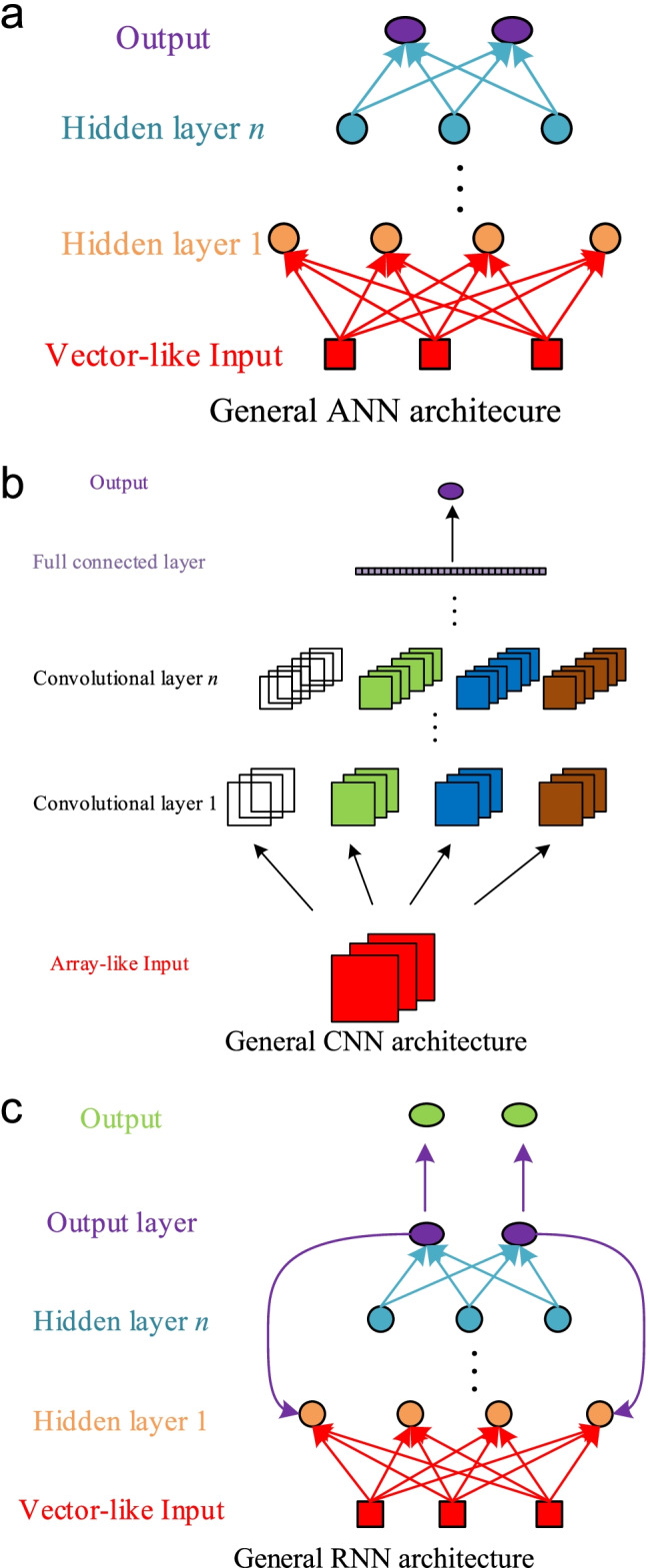
Typical schemes of ANN, CNN, and RNN models. a General ANN architecture, b general CNN architecture, and c general RNN architecture (Yu et al. 2022).

© 2021 Wiley Periodicals LLC

The MCP is a fully connected ANN, as all outputs from the previous layer are used as inputs by all neurons in the subsequent layer. Having enough layers and enough neurons, such architecture allows the MCP to interpolate any function of its inputs. However, the required number of neurons and, consequently, the number of trainable parameters might be very large, thus requiring whooping number of cases in the training dataset end enormous computational resources to tune these parameters. To limit the number of trainable parameters, a priori knowledge about structure of the input data might be used. Convolutional neural networks (CNNs, Fig. 4b) are widely used to analyze spatially distributed information. It is assumed that only data in local vicinity of each point should be considered by the model, so the neurons in the convolutional layer use only part of available data as their inputs. Another assumption is that all regions in spatial domain should be treated in the same way, thus weights and biases may be shared between groups of neurons.

ANNs considered above are stateless, as individual sets of predictors are analyzed independently. To deal with data that has internal structure of a sequence (for example, a time series data), stateful ANN architectures were suggested. In the recurrent neural networks (RNNs, Fig. 4c), the outputs of neurons are saved and then used as additional inputs. This allows the RNN to learn patterns in time series; however, with such naïve approach, the memory of the network about previous data is rather weak. To overcome this, such architectures as long short-term memory (LSTM) networks were suggested.

To get deeper into the topic of ANNs and their applications, we encourage the readers to refer to such textbooks as authored by Aggarwal (2018), Goodfellow et al. (2016), and Zhang et al. (2021). However, one should keep in mind that this area is under such a rapid development that no textbook can cover all required topics.

In the paragraphs above, we assumed the target variables to be continuous, i.e., numeric, as this is the most frequent situation in accordance with the topic of this review. However, almost all of the mentioned methods are capable to deal with categorical target variables. In this case, the regression task is replaced by the classification task, and the aim of such ML model is to predict to which class the observation belongs. This problem may be extended: the researcher might not know if there are any different classes in the dataset, and the ML model should find this out. Here, unsupervised ML methods from the cluster analysis family come to the stage (Everitt et al. 2022). Currently, these methods are not widely used in the context of this survey, so here, we do not pay much attention to them, but we suspect significant rise of interest to such techniques in the nearest future.

In this paper, we do not intend to provide exhaustive or systematic review of ML methods application for solving particular biophysical tasks. Instead, we provide a kind of general outlook of ML applications which connect optical measurements data with photosynthetic activity of higher plants and phytoplankton algae. Selected biological examples are not always representative — if there are tens or hundreds of publications implementing some particular method, we might select a random one as illustration of the approach (probably the most recent for the moment this survey prepared). To get full information, we encourage the readers to follow links in the “References” section of the cited papers. Additionally, links to systematic reviews for each section of this survey are provided.

Estimation of higher plant photosynthetic capacity and plant phenotyping from proximal reflectance data

Nowadays, a widely used in biocenosis primary productivity estimation technique is the partial least square regression (PLSR). In PLSR, the relationship between dependent and independent variables is established via latent (hidden) variables. It may be treated as a combination of the PCA with the ordinary least square (OLS) regression. While OLS regression makes hard assumptions such as no collinearity between the independent variables, PLSR allows “softening” these assumptions and making the model more reliable in real-world conditions — nevertheless being a kind of LR. Such softening proved to be robust when dealing with spectral data, especially with hyperspectral images; thus, the PLSR technique is extensively used.

In most papers mentioned below, CO₂-saturated photosynthetic rate V_c,max and the maximal rate of electron transport J_max estimated from gas exchange measurements (A/C_i curves — net CO₂ assimilation rate, A, versus calculated substomatal CO₂ concentration, C_i) were used to characterize photosynthetic capacity of plants. Such measurements were typically performed using LI-COR portable photosynthesis systems (Li-6400 and Li-6800, LICOR Biosciences, Lincoln, NE, USA). Additional information about photosynthetic capacity might be obtained from A/Q (light response — net CO₂ assimilation rate versus irradiance) curves. Leaf-level reflectance was measured with handheld spectroradiometers with typical range from VNIR (350–1000 nm) to SWIR (1000–2500 nm) spectra. Fieldspec (Analytical Spectral Devices, Boulder, CO, USA) spectroradiometers are commonly used for this purpose. Hyperspectral imagers were used to obtain reflectance data from several cropped plants or the whole canopy simultaneously.

Heckmann et al. (2017) compared the reflectance spectra (from 350 to 2500 nm) from mature leaves of representatives of 36 plant genera in order to correlate their spectral properties with the photosynthetic capacity. Both the maximal rate of carboxylation (V_c,max) and the maximal rate of electron transport (J_max) were studied. It was shown that this set of spectra was of surprisingly low diversity, with 97% of the variance contained in the first three principal components. PLSR with recursive feature elimination was selected as the best model to predict photosynthetic capacity of the species, compared to ANN approach. The authors promote leaf reflectance spectroscopy in combination with PLSR as a rapid first-pass screen to uncover variation in photosynthetic parameters in hundreds or thousands of genetically diverse individuals and to select promising lines for a more thorough analysis.

In Meacham-Hensold et al. (2019), a similar technique was applied to study the relation between spectral properties of leaves and photosynthetic activity for nine tobacco genotypes showing significant variation in photosynthetic capacity (six transgenic and three wild type lines) cultivated for 2 years. Although the PLSR model trained on the data obtained during the first year of experiment was able to accurately predict V_c,max and J_max from spectral data for plants grown during this particular year, and for genotypes included into the training dataset, its application to data collected next year and including new genotypes resulted in much poorer predictive ability. However, the model trained on data for 2 years and all genotypes showed much better predictive ability. The results suggest a need for repopulation of PLSR models annually when dealing with discreet variation in photosynthetic capacity between genotypes of a single species in crop trials. However, the extent at which models need to be repopulated in time and space for hyperspectral PLSR models is still uncertain.

In Fu et al. (2019), gas exchange and leaf reflectance data for tobacco plants were analyzed using a series of ML techniques: ANN, SVM, LASSO regression, RF regression, GPR, and PLSR. These methods were used together producing a single stacked regression (SR, also called as stacked generalization, stacking, stacking regressions, or blending) model to blend different predictors to give improved prediction accuracy. Regression stacking performed better than the individual regression techniques. Analysis of variable importance also revealed diverse abilities of the six regression techniques to utilize spectral information for the best modeling performance. It is also suggested that the stacking procedure can be further extended to harness strengths of new techniques such as the ground-based SIF system as a supplement to the hyperspectral reflectance for estimating other phenotypic traits.

Wang et al. (2021) used PLSR to predict photosynthetic capacity of maize from hyperspectral (500–2400 nm) reflectance of leafs. It was shown that the PLSR models based on spectra can provide rather good predictions of V_c,max on the leaf level, but direct upscaling of such models to canopy, regional or global scale may be unreliable, and physically based radiative transfer models (RTMs) may be preferred. To improve scalability of ML models, an indirect approach to predict photosynthetic capacity is suggested: spectra are used to predict leaf traits, and the final prediction is based on these traits but not the raw spectral data.

In Fu et al. (2020), the aforementioned ground-based phenotyping platform with hyperspectral imager was used to study photosynthetic capacity of tobacco plants. Image preprocessing was performed by k-means cluster analysis, which separated the pixels into six groups: sunlit leaves, shaded leaves, shadow, box, calibration panel, and soil. It was shown that both V_c,max and J_max can be predicted by PLSR from spectral data with coefficient of determination R² ~ 0.8, which is much higher than R² for RTM (~ 0.6). Application of spectral indices (simple ratios of reflectance at two wavelength or more complicated combinations of reflectance at three wavelengths) slightly increased R² for V_c,max leaving R² for J_max unchanged. Further analysis on spectral resampling revealed that V_c,max and J_max could be predicted with ~ 10 spectral bands at a spectral resolution of less than 14.7 nm.

A modified version of the ground-based phenotyping platform with two hyperspectral imagers was used in Meacham-Hensold et al. (2020). Additionally, leaf-level spectral measurements were made using a handheld spectroradiometer in range from 400 to 2500 nm. Photosynthetic capacity was estimated from gas exchange measurements using both A/C_i and A/Q curves, so an extended set of functional parameters (V_c,max, maximum electron transport rate in particular conditions, J₁₈₀₀; maximal light-saturated photosynthesis, P_max) was analyzed. Comparison of PLSR models using spectral data in the whole range and using VNIR spectra only showed that SWIR data did not improve predictions of photosynthetic capacity. The best predictions were obtained for V_c,max (R² = 0.79), while R² for J₁₈₀₀ and P_max was below 0.6.

Song and Wang (2021) used ANN approach to study the relation between Japanese beech Fagus crenata leaf reflectance and their photosynthetic capacity. The networks had seven hidden layers and an output layer with a single neuron which output was considered V_c,max or J_max prediction. The authors conclude that ANN is a feasible approach for predicting leaf functions from reflectance spectra; however, the coefficients of correlation obtained by the best models are rather low, which agrees to Heckmann et al. (2017) results. The readers may refer to the survey by Kamilaris and Prenafeta-Boldú (2018) on deep learning in agriculture for more examples of ANN applications in this field.

Kumagai et al. (2022) compared PLSR, LASSO, RR, and SVR methods to predict photosynthetic capacity of soybean from hyperspectral images under in-field canopy warming. PLSR, RR, and SVR models outperformed the LASSO regression model. However, despite having a relatively small sacrifice in accuracy, in this study, LASSO provided information on which spectral bands are most important for photosynthetic capacity prediction. Overall, compared with PLSR commonly used in the previous studies, no improvements in the accuracy, linearity, and sensitivity were obtained by RR, LASSO, or SVR. Hyperspectral reflectance can capture rapidly and accurately photosynthetic biochemical acclimation to increased temperature in the field, greatly enhancing our ability to assess the impact of future warming on ecosystem productivity.

As a short digest, we may conclude that all of the cited papers present just proof-of-the-concept for applicability of ML methods for estimation of photosynthetic capacity rather than any valuable biological result. Among other methods, PLSR seems to be the most reliable, although its performance may be improved by combining with other methods using SR technique. Large-scale data harvesting may lead to significant improvement in prediction ability of ML models, so we may expect to generate high-quality ML models suitable for real applications in the coming few years.

Crop yield prediction and estimation of land biocenoses gross primary productivity from satellite and airborne spectral imaging

Crop yield prediction is important for precision agriculture; thus, there are numerous publications on the topic, and a wide variety of ML methods is used. In the previous section, most models were built to treat one-dimensional spectral data, and rather simple regression techniques such as PLSR showed good performance. Even if spectral imagers were used, each spatial channel was processed separately, and changes of acquired spectra in temporal domain were neglected by the models. Although the same approach may be used for the analysis of satellite and airborne (hyper/multi)spectral images, models which take into account spatial distribution and temporal changes in spectral data might show significantly better performance. In this case, the model input may be considered four-dimensional, having two spatial dimensions, one spectral dimension, and one temporal dimension. To treat such multidimensional data, several advanced ANN-based approaches were suggested. These approaches utilize convolutional neural network (CNN) solely or in combination with recurrent neural networks (RNNs), such as LSTM networks. Below we will consider several single-dimensional and multidimensional models suggested for analysis of satellite and airborne spectral images. The reader may find more examples in van Klompenburg et al. (2020) review on the application of ML methods for crop yield prediction. Another noteworthy review on this topic was published by Chlingaryan et al. (2018).

As for one-dimensional models, Wang et al. (2020) used PLSR to predict foliar traits from the airborne imaging data from the aforementioned NEON AOP dataset. Although in this paper authors did not register photosynthetic activity directly, good predictions were obtained for such photosynthesis-related parameters as chlorophyll, carotenoid and starch content, leaf mass per area, etc. Guan et al. (2017) applied the PLSR approach to analyze optical, fluorescence, thermal, and microwave satellite data to estimate large-scale crop yields. Seasonal changes in wide spectral range were studied for various regions of the USA from year 2002 to 2009. Additionally, climate data was considered auxiliary input of the model. Statistical data from the National Agricultural Statistics Service of the US Department of Agriculture (USDA) was used to derive county-level net primary production of crops. PLSR was used to evaluate relationships between crop yield and the satellite-derived metrics and climate variables. It was shown that PLSR was suitable for this task, and the 1st component achieved 82% of the optimal model performance, while additional components captured the remaining 18% of the performance. The interpretation of individual components was discussed.

Setiyono et al. (2018) used nonlinear GPR to obtain leaf area index (LAI) from a combined time series of the 250-m spatial resolution surface reflectance in four spectral bands — blue (459–479 nm), red (620–670 nm), near infrared (841–876 nm), and middle infrared (2105–2155 nm) from MODIS satellites (TERRA and AQUA). LAI expresses the leaf area per unit ground surface area of a plant and is commonly used as an indicator of the growth rate of a plant. Multitemporal LAI maps were used for rice yield simulation for eight rice-producing provinces in Vietnam. Simulation results were in good agreement with official government-reported yield.

Shiu and Chuang (2019) compared the performance of LR and SVR with the local geographically weighted regression (GWR) for rice yield prediction from multispectral images of two counties of Taiwan with four spectral bands (blue 455–525 nm, green 530–590 nm, red 625–695 nm, and near-infrared 760–890 nm) and 6-m spatial resolution obtained from SPOT-7 satellite. Several spectral indices were evaluated as model inputs together with original bands. The yield data contained ground survey data and total yield data acquired from the official statistical reports published by Taiwan’s Agriculture and Food Agency. It was shown that the results of the GWR model, which takes into account spatial information, were the most suitable.

You et al. (2017) suggested histogram-based approach to pre-processing multispectral images. It was assumed that only the number of different pixel types in an image was informative, but not the positions of individual pixels. Thus, they compressed a time series of multispectral images into 3D histograms, having one spectral, one temporal, and one intensity (“bin”) dimension. 3D histograms were used as inputs of CNN and LSTM networks for the prediction of yearly average soybean yields at the county-level. Spatio-temporal information was explicitly used by Gaussian process (GP) model assuming that the errors corresponding to data points that are spatially closer tend to vary less. Model results obtained from MODIS satellite images (7 surface reflectance bands and 2 surface temperature bands) were compared to publicly available data from the USDA. CNN model outperformed LSTM model and other regression models, and application of GP correction to both LSTM and CNN models improved their predictive ability. The importance of individual spectral bands for accurate crop yield prediction was discussed.

Russello (2018) in her MSc thesis suggested 3D spatio-temporal CNN architecture, in which convolution is performed in both spatial and temporal domains. Time series consisting of 24 daily MODIS satellite images (7 surface reflectance bands, 2 surface temperature bands, and binary cropland mask) was used as model input. The predictive ability of the suggested model was better compared to the aforementioned histogram-based model (Russello 2018).

Nevavuori et al. (2019) applied 2D CNNs to build a model for crop (wheat and barley) yield prediction based on the red–green–blue (RGB) and the normalized difference vegetation index (NDVI) data with spatial resolution of 0.3125 m acquired by unmanned aerial vehicles (UAVs) in the vicinity of the city of Pori in Finland. The images were taken at different growth phases of the crop. The yield data was acquired at the end of vegetation from measurement devices attached to harvesters. Complex network architecture with several convolution, batch normalization, max pooling, and fully connected layers was borrowed from networks designed for image classification tasks. It was shown that the best-performing model can predict within-field yield with a mean absolute error of 484 kg/ha (8.8%) based only on RGB images in the early stages of growth (< 25% total thermal time). The model for RGB images at later growth stage returned higher error values (680 kg/ha, 12.6%).

Fernandez-Beltran et al (2021) promote a 3D spatio-temporal CNN to estimate rice yield in Nepal from multispectral images obtained by Sentinel-2 satellite. Images obtained at the start, the peak, and the end of the season are used as model inputs. Climate and soil maps are used as auxiliary inputs. Predictive ability of the proposed model was compared to other approaches, such as LR, RR, SVR, GPR, and other previously suggested 2D CNN and 3D CNN architectures. The extensive experiments conducted in this work demonstrate the suitability of the proposed CNN-based framework for rice crop yield estimation. It was shown that simultaneous analysis of several images taken at different stages of crop cultivation allows substantial improvement to the rice crop classification accuracy as opposed to the use of single time period images.

Qiao et al. (2021) suggested spatial-spectral-temporal neural network (SSTNN) architecture (Fig. 5), in which 3D CNN was used to acquire the joint spatial-spectral features from each multispectral image, and RNN consisting of several bidirectional LSTM cells was used to analyze temporal dynamics. MODIS 7-band multispectral images were used as model inputs; and the yield predictions for winter wheat and corn for several regions of China were compared to statistical data from the Agricultural Statistic Yearbook and Resource Discipline Innovation Platform. It was found that the SSTNN achieved satisfactory performance 2 months before harvest in the wheat yield prediction and 3 weeks in the corn prediction.

Fig. 5.

Overview of the proposed SSTNN. Reprinted from International Journal of Applied Earth Observation and Geoinformation, Vol. 102, Qiao et al., Crop yield prediction from multi-spectral, multi-temporal remotely sensed imagery using recurrent 3D convolutional neural networks, 102,436,

© 2021, with permission from Elsevier

Jiang et al. (2021) worked out a long-term and real-time SatelLite Only Photosynthesis Estimation (SLOPE) gross primary productivity (GPP) product covering the contiguous USA. Four different ML methods (LASSO regression; multivariate adaptive regression splines, MARS; k-nearest neighbor regression, KNN; and RF regression) are used to estimate photosynthetically active radiation (PAR) from MODIS satellite images. Estimated PAR values together with near-infrared reflectance of vegetation (NIR_V) indices are used to calculate GPP. Evaluation against AmeriFlux ground-truth GPP based on eddy covariance measurements shows that the SLOPE GPP product has a reasonable accuracy, with an overall R² of 0.85 and root mean square error of 1.63 gCm⁻²d⁻¹.

The FLUXCOM initiative (http://www.fluxcom.org/) aims to provide an ensemble of machine learning–based global flux products to the scientific community for assessing biosphere–atmosphere carbon and energy fluxes over large regions. In total, FLUXCOM uses up to 11 algorithms from four broad families: tree-based methods (RF regression and model tree ensembles, MTE), regression splines (MARS), neural networks (ANN and group method of data handling, GMDH), and kernel methods (SVR; kernel ridge regression, KRR; and GPR). An overview of this approach may be found in Jung et al. (2020), and technical details about algorithms used — in Tramontana et al. (2016).

The ML applications considered in this section are probably the most sophisticated and mature among other approaches reviewed in this survey. Advanced ANN architectures using spatio-temporal variation of input data for plant productivity prediction in general outperformed other regression methods. As in the previous section, here, we may see that the combination of different ML methods may improve the prediction quality. Although most of the considered models are the proof-of-concept models used for evaluation of different ML techniques for plant productivity prediction, several ready-to-use products are already available.

Water quality assessment and estimation of chlorophyll a content from proximal and satellite spectral imaging

A wide range of ML methods was evaluated for assessment of water quality and estimation of primary productivity of aquatic systems. In the case of aquatic biocenoses, chlorophyll a (Chl-a) content is commonly used for the estimation of phytoplankton biomass. Traditional method to derive Chl-a content from reflectance spectra assumes calculation of some spectral indices, which are then used for the calculation of Chl-a content via polynomial or other approximation of empirical dependency. ML is expected to improve accuracy of such calculations.

Maier et al. (2018) used RF regression to estimate Chl-a content in The River Elbe in Germany from proximal hyperspectral data (125 bands in range from 450 to 950 nm) measured within a 70° angle towards the water surface. It was shown that applying PCA to reduce the dimensionality of RF regression model input data to 20 principle components improves its performance.

Camps-Valls et al. (2006) compared the relevance vector regression (RVR) and SVR approaches to prediction of Chl-a content in marine water from SeaStar (OrbView-2) satellite multispectral data. Both methods showed similar performance and outperformed traditional methods. Blix et al. (2018, 2019) developed GPR model for the prediction of Chl-a content and other water quality parameters for inland and ocean waters from Sentinel-3 data. Models taking into account all spectral bands and 3 or 5 bands selected by the automatic model selection algorithm were considered. It was shown that the best performance was obtained for model using three reflectance bands centered at 442.5, 665, and 681.25 nm.

Li et al. (2021) compared LR, SVR, and Catboost regression for the prediction of the Chl-a content in 45 lakes in China from Sentinel-2 multispectral images. Additionally, spectral data was used to classify the water bodies by three groups with different content of total suspended matter (TSM) and dissolved organic carbon (DOC). It was shown that all three studied regression methods outperformed traditional Chl-a content calculation methods. SVR regression was considered to give an optimum performance (R² > 0.88 results of calibration and validation; and fitted equation closed to 1:1 line) compared to other regression algorithms. Zhao et al. (2021) showed that ANN approach (three different network architectures were tested) outperforms LR approach in Chl-a content prediction in Taihu Lake, China, from multispectral images from Landsat-8 satellite.

Graban et al. (2020) used the ANN approach to estimate Chl-a concentration from the spectral particulate beam-attenuation coefficient data collected during numerous expeditions all over the world. The multi-layer perceptron with two hidden layers allowed accurate estimation of Chl-a content using three spectral bands in the red spectral region (664–670 nm, 682–688 nm, and 704–710 nm). Asim et al. (2021) proposed the ocean color net (OCN) ANN consisting of fully connected and batch normalization layers for the prediction of Chl-a content in the Barents Sea from Sentinel-r multispectral images. The suggested model outperformed other ML methods having GPR as the closest competitor.

Hafeez et al. (2019) compared several machine learning techniques — ANN, RF regression, cubist regression, and SVR, for the estimation of Chl-a content and other water quality parameters in optically-complex (case 2) marine waters near Hong Kong. Landsat-(5,7,8) reflectance data were compared with in situ reflectance data to evaluate the performance of ML models. The highest accuracies of the water quality indicators were achieved by ANN for both in situ and satellite reflectance data. The importance of individual spectral bands for accurate predictions was considered.

Pahlevan et al. (2020, 2022) and Smith et al. (2021) used the mixture density network (MDN, Fig. 6) approach to predict Chl-a content and other water quality indicators (content of total suspended solids, TSS and colored dissolved organic matter, CDOM) for inland and coastal waters from the Landsat-8, Sentinel-2, and Sentinel-3 data. MDN is a specialized ANN architecture intended to deal with uncertainty in predicted data by calculating several estimations together with their uncertainties and likelihood values, and then selecting the most probable one as the final estimation. Suggested model outperformed traditionally used Chl-a content calculation methods. Different methods of atmospheric correction for image preprocessing are considered.

Fig. 6.

Schematic block diagram illustrating the main components of a mixture density network (MDN), a class of neural networks that estimates multivariate probability density functions with their corresponding parameters (μ, Σ) and mixing coefficients (α) to arrive at an optimal Chla retrieval. Note that a covariance matrix (Σ) is reduced down to standard deviation (σ) when a single target variable (e.g., Chla) is sought. Reprinted from Remote Sensing of Environment, Vol. 240, Pahlevan et al., Seamless retrievals of chlorophyll-a from Sentinel-2 (MSI) and Sentinel-3 (OLCI) in inland and coastal waters: a machine-learning approach, 111,604,

© 2020, with permission from Elsevier

Although many different ML methods showed reasonable performance in water quality assessment, it looks like the ANN-based approaches tend to outperform both the traditional spectral indices-based methods and other ML methods. The reader may refer to Hassan and Woo (2021) to find an annotated list of 113 publications devoted to the application of ML methods for water quality assessment using satellite data.

Improving primary productivity estimates using solar-induced chlorophyll fluorescence data

Fluorescence is emitted by chlorophyll molecules which are directly involved into the process of photosynthesis, so it is natural to assume that taking it into account along with reflectance data should improve primary productivity estimates from remote measurements. However, chlorophyll fluorescence is strongly re-absorbed; thus, the relation between its measured intensity and photosynthetic activity of plants may be very nonlinear. Thus, significant efforts have been made to scale the relation between fluorescence and photosynthesis from subcellular to leaf, canopy, and regional level.

Verrelst et al. (2016) used simulation data generated by the soil canopy observation, photochemistry and energy fluxes (SCOPE) model to train LR and GPR models intended to derive net photosynthesis of the canopy (NPC) from the SIF data. To analyze the influence of biochemistry, leaf and canopy mechanisms impacting the SIF signal, multiple canopy configurations were simulated. It was shown in heterogeneous conditions; the maximum carboxylation capacity at optimum temperature, chlorophyll content, and canopy structural variables (e.g., LAI) are the key variables affecting SIF–NPC relationships.

Liu et al. (2019) used an empirical approach based on RF regression to predict the SIF escape probability from leaf level to canopy level and from photosystem level to canopy level using the red, red-edge, and far-red anisotropic reflectance information. The SCOPE model simulations were employed for the training of the RF. The performance of the SIF downscaling method was evaluated with SCOPE and discrete anisotropic radiative transfer (DART) model simulations, ground measurements, and airborne data. It was shown that estimated SIF at the photosystem level matched well with simulated reference data, and the relationship between SIF and PAR absorbed by chlorophyll was improved by SIF downscaling. The authors suggested the downscaling of canopy SIF as an efficient strategy to normalize species-dependent effects of canopy structure and varying solar-view geometries and to improve estimates of photosynthesis using remote sensing measurements of SIF.

Zhang et al. (2018) used a rather simple ANN to discover the relation between SIF measured by OCO-2 and surface reflectance data from MODIS instruments. This allowed generation of a global spatially contiguous solar-induced fluorescence (CSIF) datasets. The clear-sky instantaneous CSIF showed high accuracy against the clear-sky OCO-2 SIF and little bias across biome types. The all-sky daily average CSIF dataset exhibited strong spatial, seasonal, and interannual dynamics that were consistent with daily SIF from OCO-2 and GOME-2. Another ANN-based SIF product based on OCO-2 and MODIS data was suggested by Yu et al. (2019). A similar approach taking GOME-2 data as a reference was used by Gentine and Alemohammad (2018).

Wen et al. (2020) compared RF and ANN approaches to downscaling coarse-resolution SIF data from GOME-2 and SCIAMACHY on the basis of high-resolution MODIS surface reflectance data. RF and ANN showed similar prediction performance. A powerful feature with RF was that model uncertainty could be simultaneously quantified based on the bootstrapped trees without additional computational cost. There is no established procedure that is mature and accurate to be applied to quantify the uncertainty for ANN-based prediction, so RF approach was selected to generate downscaled data.

Peng et al. (2020) evaluated five ML algorithms (LASSO, RR, SVR, RF regression, and ANN) for maize and soybean yield prediction with both remote-sensing-only and climate-remote-sensing-combined variables. High-resolution SIF products from OCO-2 and TROPOMI outperformed coarse-resolution GOME-2 SIF product in crop yield prediction. However, using currently available high-resolution SIF products did not guarantee consistently better yield prediction performances than using other satellite-based remote sensing variables in all the evaluated cases. The nonlinear algorithms (RF regression, SVR, and ANN) performed better than the linear algorithms (LASSO and RR). LASSO and RR performed similarly, and the three nonlinear algorithms achieved similar performances in yield prediction.

Detection of unfavorable environmental conditions and plant diseases, and the prediction of algal bloom from optical measurements data

Several ML-based approaches were suggested for the detection of various stressors disturbing photosynthetic processes. Most of them use chlorophyll a fluorescence transients as the main data source. Deficiency of nutrients and water deficiency, poisoning by herbicides and heavy metals, and infection with diseases have been considered, and various types of ML approaches were evaluated.

Goltsev et al. (2012) evaluated ANN approach to estimate relative water content (RWC) in bean plant leaves from PF, DF, and MR of light at 820 nm signals. Three types of data were used as model inputs: the complete induction curves of PF, DF, or MR, and their combination, JIP test parameters derived from PF curves, and DF curve parameters. PC transformation of the experimental data was performed, and the principal components whose contribution to the total variation was larger than 0.05% were used as ANN inputs. It was shown that the models trained on complete PF and DF curves (separately or together) performed robustly with R² greater than 0.9, but neither MR traces nor JIP test nor parameters of the DF curves contained enough information for the accurate prediction of RWC.

Rybka et al. (2019) performed screening of JIP test parameter combinations suitable for the prediction of water deficiency by ANN-based model. The best model consisted of three inputs: maximal quantum yield of photosystem 2 (PS2) photochemistry, approximated number of active PS2 reaction centers per absorption, and measure of forward electron transport, three hidden nodes, and one output (WSD), and the provided precision was 82% with a correlation coefficient of 0.98.

Spyroglou et al. (2021) uses beta-generalized linear mixed model (GLMM) along with a beta-generalized estimating equation (GEE) model for quantitative estimation of water status in field-grown wheat plants from JIP test parameters. The performance of the beta GLMM showed that it can be a very useful tool for predicting RWC of plant tissues.

Kalaji et al. (2018) used super-organizing maps (sSOM) approach to find a connection between mineral content of soil and plant leaves and the activity of photosynthetic machinery assessed by chlorophyll a fluorescence signals. A self-organizing map (SOM) is an ANN-based unsupervised ML technique used to produce a low-dimensional representation of a higher-dimensional data set while preserving its topological structure. sSOM is an extension of SOM to multiple data layers. In this study, PCA in combination with hierarchical k-means cluster analysis was used to group samples by their chemical composition. Five groups of patterns in the chlorophyll fluorescent parameters were established: the “no deficiency,” Fe-specific deficiency, slight, moderate, and strong deficiency. sSOM with one layer representing JIP test parameters and separate layers representing each of the studied minerals allowed characterization of each previously established group by the parameters pf photosynthetic activity.

Bluementhal et al. (2014, 2017, 2020) used both supervised and unsupervised Hidden Markov Models (HMM) for the classification of plant stress types and levels from chlorophyll fluorescence video imaging data. The action of drought, nutrient deficiency, and herbicide stress was studied. Aleksandrov (2022) created ANN which takes PF data as input and outputs a six-component vector with components indicating Fe, K, N, P, and Ca deficiencies and no deficiency (control plants). The model provides rather good performance to identify single nutrient deficiency.

Here, we will omit discussing if the nitrogen content in plants can be reliably predicted from proximal and remote reflectance data or not, as it is out of scope of this review. However, we should mention Du et al. (2016) paper, where the authors evaluated whether photosynthetic-activity-related LIF data might improve leaf nitrogen content (LNC) prediction. Four regression algorithms (SVR, PLSR, and two variants of ANN) were used to estimate rice LNC based on combination of reflectance and LIF spectra. It was shown that training the LNC models with only the reflectance data allowed obtaining R² higher than 0.95, and the improvement of R² in the LNC estimation models taking into account LIF spectra was not evident. The radial basic function ANN outperformed the other considered methods.

Weng et al. (2021) suggested the least squares SVM (LS-SVM) for rapidly detecting Citrus greening disease (Huanglongbing) from JIP test parameters. The results suggested that the main disturbances of photosynthetic structure and function in Huanglongbing-infected leaves were associated with impairment of energetic connectivity of antennae in PS2, dysfunction of oxygen-evolving complex, and inhibition of the primary PS2 electron acceptor (Q_A^–) reoxidation. The suggested LS-SVM model achieved overall Huanglongbing disease detection accuracies of over 95%.

Wahabzada et al. (2015, 2016) present a cascade of data mining techniques for fast and reliable data-driven sketching of complex hyperspectral dynamics in plant science and plant phenotyping. In Wahabzada et al. (2015), simplex volume maximization (SiVM) is used to automatically discover archetypal hyperspectral signatures that are characteristic for particular diseases. Wahabzada et al. (2016) suggested the “wordification” approach to hyperspectral image analysis based on latent Dirichlet allocation. It was demonstrated that one can track automatically the development of three foliar diseases of barley.

Marques da Silva et al. (2020) applied several ML algorithms (k-nearest neighbors, decision trees, ANNs, genetic programming) to PF recorded in different species and cultivars of vine grown in the same environmental conditions. The phylogenetic relations between the selected Vitis species and Vitis vinifera cultivars were established with molecular markers. Both ANN (71.8%) and genetic programming (75.3%) presented much higher global classification success rates than k-nearest neighbors (58.5%) or decision trees (51.6%), genetic programming performing slightly better than ANN.

Duarte et al. (2021) used the linear discriminant analysis to create a toxicophenomic OPTOX index unifying all the fluorescence data provided by the chlorophyll a induction curve (PF). The index proved to be an efficient tool for ecotoxicological assays with marine model diatoms and evidenced a high degree of reliability for classifying the exposure of the cells to emerging contaminants.

Khruschev et al. (2021) compared two ANNs supposed to predict the unfavorable influence of heavy metals on phytoplankton from fluorescence data. The first one took unprocessed fluorescence transients as the inputs, and the other — JIP test parameters. It was shown that the predicting ability of these two ANNs was almost equal, but the number of internal model parameters of the first model was substantially greater compared to the second one. Thus, the second model should be preferred as less number of samples is required for its training.

Liu et al. (2020) suggested an ANN model optimized by genetic algorithm for rapid in situ measurements of algal cell concentrations. The model uses fluorescence spectrum as input and allows monitoring of the Chlamydomonas reinhardtii cell concentrations in the range from 2∙10⁵ to 6.4∙10⁶ cells∙mL⁻¹. Blue (470 nm) LED was used for fluorescence excitation. It was shown that application of genetic algorithm to find the optimal initial weights and thresholds of the network reduced the mean absolute error by an order of magnitude (from 1.2∙10⁵ cells∙mL⁻¹ for the ANN without optimization to 1.4∙10⁵ cells∙mL⁻¹ for the optimized ANN).

Eze et al. (2021) proposed a forecasting model for the high accuracy prediction of chlorophyll a content to enable aquafarm managers to take remediation actions against the occurrence of toxic algal blooms in the aquaculture industry. The proposed model combines the ensemble empirical mode decomposition (EEMD) technique and a deep learning LSTM neural network. The water quality model takes as its input fluorescence measured by a TriLux 2000 multi-parameter fluorometer and excited at 470 nm (Chl-a) and 530 nm (phycoeretrin). Light scattering due to media turbidity is considered at 685 nm. The model was built on water quality sensor data collected from the Loch Duart salmon aquafarm in Scotland and provided high prediction accuracy.

Almuhtaram et al. (2021) evaluated several ML algorithms for anomaly detection in cyanobacterial fluorescence signals from phycocyanin and chlorophyll a fluorescence signals measured using YSI EXO2 (YSI, Yellow Springs, OH, USA) multiparameter water quality sondes equipped with total algae sensors. These sensor measure fluorescence exited at 470 nm (Chl-a) and 590 nm (phycocyanin). Four widespread and open source algorithms were evaluated on data collected at four buoys in Lake Erie from 2014 to 2019: local outlier factor (LOF), One-Class SVM, elliptic envelope, and Isolation Forest (iForest). The One-Class SVM and elliptic envelope models both achieve a maximum average F1 score of 0.86 among the four datasets.

Concluding remarks

A wide range of ML techniques has been evaluated to establish connection between optical measurement data and the activity of photosynthetic apparatus of plants and phytoplankton. We can see that in some cases (for example, when dealing with reflectance spectra of individual plant leafs), rather simple linear methods, such as PLSR, outperform more sophisticated ML approaches like ANN. This may be related to the number of internal degrees of freedom (i.e., fitted parameters) of the model: the more sophisticated model has more parameters to fit than a simpler one, so in general, we need to have more samples in the training dataset for the sophisticated model to achieve the same predictive ability. However, this is true only if the interrelation between model inputs and predicted variables is simple enough to be robustly reproduced by the simple model. When dealing with complex nonlinear relations, state-of-the-art ML methods significantly outperform simple regression technique. The ability of ANN-based methods to combine different types of data sources and take into account spatial and temporal variation of data makes such approaches unbeatable for the analysis of time series of satellite and airborne hyperspectral images.

The area for ML application in biological research, ecological monitoring, agriculture, and biotechnology is rapidly growing. Most of the papers included into this survey do not provide any valuable biological results but present proof-of-concept for further development of ML-based methods in various new fields of knowledge. However, there are several mature ML-based products that can be readily used for both scientific research and agricultural applications. Most of these products are based on spatio-temporal analysis of satellite images, and they provide the researcher with essential data unavailable by other means. Here, we may highlight the SLOPE gross primary productivity product (Jiang et al. 2021) and the FLUXCOM initiative (Jung et al. 2020). In the nearest future, we expect the number of such ready-to-use products to increase, and their coverage to grow. Rapid increase in the data availability will allow creation of new state-of-the-art models for ecological monitoring, water quality assessment, and other important practical tasks.

Abbreviations

A

Net CO₂ assimilation rate

ANN

Artificial neural network

CDOM

Colored dissolved organic matter

Chl-a

Chlorophyll a

C_i

Calculated substomatal CO₂ concentration

CNN

Convolutional neural network

CSIF

Contiguous solar-induced fluorescence

DART

Discrete anisotropic radiative transfer

DF

Delayed fluorescence

DOC

Dissolved organic carbon

EEMD

Ensemble empirical mode decomposition

ESA

European Space Agency

ETC

Electron-transport chain

FIRe

Fluorescence induction and relaxation

GEE

Generalized estimating equations

GLMM

Generalized linear mixed model

GMDH

Group method of data handling

GOME-2

Global Ozone Monitoring Experiment-2

GP

Gaussian process

GPP

Gross primary productivity

GPR

Gaussian process regression

GWR

Geographically weighted regression

HMM

Hidden Markov model

J₁₈₀₀

Maximum electron transport rate in particular conditions

JIP test

See Kalaji et al. (2017) for details

J_max

Maximal rate of electron transport

KNN

K-nearest neighbor

KRR

Kernel ridge regression

LAI

Leaf area index

LASSO

Least absolute shrinkage and selection operator

LED

Light-emitting diode

LIF

Laser induced fluorescence

LNC

Leaf nitrogen content

LOF

Local outlier factor

LR

Linear regression

LS-SVM

Least squares support vector machine

LSTM

Long short-term memory

MARS

Multivariate adaptive regression splines

MDN

Mixture density network

ML

Machine learning

MLP

Multilayer perceptron

MODIS

Moderate resolution imaging spectroradiometer

MR

Modulated reflection

MSE

Mean squared error

MTE

Model tree ensembles

NASA

National Aeronautics and Space Administration

NDVI

Normalized difference vegetation index

NEON AOP

National Ecological Observatory Network Airborne Observation Platform

NIR

Near-infrared

NIRV

Near-infrared reflectance of vegetation

NPC

Net photosynthesis of the canopy

O₂–A and O₂–B

Molecular oxygen Fraunhofer absorption bands

OCN

Ocean color net

OCO-2

Orbiting Carbon Observatory-2

OLCI

Ocean and Land Colour Instrument

OLS

Ordinary least square

P700

Photosystem I reaction center pigment

PAM

Pulse-amplitude-modulation

PAR

Photosynthetically active radiation

PCA

Principal components analysis

PF

Prompt fluorescence

PLSR

Partial least square regression

P_max

Maximal light-saturated photosynthesis

PS2

Photosystem 2

Q

Irradiance

Q_A^–

Primary PS2 electron acceptor

R²

Coefficient of determination

RF

Random forest

RGB

Red–green–blue

RNN

Recurrent neural network

RR

Ridge regression

RTM

Radiative transfer model

RVM

Relevance vector machine

RVR

Relevance vector regression

RWC

Relative water content

SCOPE

Soil canopy observation, photochemistry and energy fluxes

SIF

Solar-induced chlorophyll fluorescence

SIMD

Single instruction multiple data

SiVM

Simplex volume maximization

SLOPE

SatelLite Only Photosynthesis Estimation

SLSTR

Sea and land surface temperature radiometer

SOM

Self-organizing map

SR

Stacked regression

sSOM

Super-organizing maps

SSTNN

Spatial-spectral-temporal neural network

SVM

Support vector machine

SVR

Support vector regression

SWIR

Short wave infrared spectral range

TSM

Total suspended matter

TSS

Total suspended solids

UAV

Unmanned aerial vehicle

USDA

United States Department of Agriculture

USGS

United States Geological Survey

V_c,max

CO₂-saturated photosynthetic rate

VNIR

Visible/near infrared

Funding

This research was carried out as part of the Scientific Project of the State Order of the Government of Russian Federation to Lomonosov Moscow State University No. 121032500060–0 with partial support by the Russian Foundation for Basic Research (project 20–04–00465) and the Russian Science Foundation (project 20–64–46018).

Declarations

Ethics approval

Not applicable.

Consent to participate

Not applicable.

Consent for publication

Not applicable.

Competing interests

The authors declare no competing interests.

References

- Aggarwal CC (2018) Neural networks and deep learning. a textbook. Springer Cham. XXIII. 10.1007/978-3-319-94463-0
- Aguirre M, Berruti B, Bezy J-L, Drinkwater M, Heliere F, Klein U, Mavrocordatos C, Silvestrin P, Greco B, Benveniste J. Sentinel-3 - the ocean and medium-resolution land mission for GMES operational services. ESA Bull. 2007;131:24–29. [Google Scholar]
- Aleksandrov V. Identification of nutrient deficiency in plants by artificial intelligence. Acta Physiol Plant. 2022;44:29. doi: 10.1007/s11738-022-03363-0. [DOI] [Google Scholar]
- Almuhtaram H, Zamyadi A, Hofmann R. Machine learning for anomaly detection in cyanobacterial fluorescence signals. Water Res. 2021;197:117073. doi: 10.1016/j.watres.2021.117073. [DOI] [PubMed] [Google Scholar]
- Antal T, Konyukhov I, Volgusheva A, Plyusnina T, Khruschev S, Kukarskikh G, Goryachev S, Rubin A. Chlorophyll fluorescence induction and relaxation system for the continuous monitoring of photosynthetic capacity in photobioreactors. Physiol Plant. 2019;165:476–486. doi: 10.1111/ppl.12693. [DOI] [PubMed] [Google Scholar]
- Antal TK, Venediktov PS, Matorin DN, Ostrowska M, Woźniak B, Rubin AB. Measurement of phytoplankton photosynthesis rate using a pump-and-probe fluorometer. Oceanologia (poland) 2001;43(3):291–313. [Google Scholar]
- Asim M, Brekke C, Mahmood A, Eltoft T, Reigstad M. Improving chlorophyll-a estimation from Sentinel-2 (MSI) in the Barents Sea using machine learning. IEEE J Select Topics Appl Earth Observations Remote Sens. 2021;14:5529–5549. doi: 10.1109/JSTARS.2021.3074975. [DOI] [Google Scholar]
- Bacon F, Fowler T. Novum organum. Oxford: Clarendon Press; 1889. p. 629. [Google Scholar]
- Baldocchi DD, Hincks BB, Meyers TP. Measuring biosphere-atmosphere exchanges of biologically related gases with micrometeorological methods. Ecology. 1988;69:1331–1340. doi: 10.2307/1941631. [DOI] [Google Scholar]
- Blix K, Pálffy K, Tóth VR, Eltoft T. Remote sensing of water quality parameters over Lake Balaton by using Sentinel-3 OLCI. Water. 2018;10(10):1428. doi: 10.3390/w10101428. [DOI] [Google Scholar]
- Blix K, Li J, Massicotte P, Matsuoka A. Developing a new machine-learning algorithm for estimating chlorophyll-a concentration in optically complex waters: a case study for high northern latitude waters by using Sentinel 3 OLCI. Remote Sens. 2019;11(18):2076. doi: 10.3390/rs11182076. [DOI] [Google Scholar]
- Blumenthal J, Megherbi DB, Lussier R (2014) Unsupervised machine learning via Hidden Markov Models for accurate clustering of plant stress levels based on imaged chlorophyll fluorescence profiles & their rate of change in time. 2014 IEEE International Conference on Computational Intelligence and Virtual Environments for Measurement Systems and Applications (CIVEMSA). 76–81. 10.1109/CIVEMSA.2014.6841442
- Blumenthal J, Megherbi DB, Lussier R (2017) Supervised machine learning via Hidden Markov Models for accurate classification of plant stress levels & types based on imaged Chlorophyll fluorescence profiles & their rate of change in time. 2017 IEEE International Conference on Computational Intelligence and Virtual Environments for Measurement Systems and Applications (CIVEMSA). 211–216. 10.1109/CIVEMSA.2017.7995328
- Blumenthal J, Megherbi DB, Lussier R. Unsupervised machine learning via Hidden Markov Models for accurate clustering of plant stress levels based on imaged chlorophyll fluorescence profiles & their rate of change in time. Comput Electron Agric. 2020;174:105064. doi: 10.1016/j.compag.2019.105064. [DOI] [Google Scholar]
- Bovensmann H, Burrows JP, Buchwitz M, Frerick J, Noël S, Rozanov VV, Chance KV, Goede APH. SCIAMACHY: mission objectives and measurement modes. J Atmos Sci. 1999;56(2):127–150. doi: 10.1175/1520-0469(1999)056<0127:SMOAMM>2.0.CO;2. [DOI] [Google Scholar]
- Bukhov N, Egorova E, Krendeleva T, Rubin A, Wiese C, Heber U. Relaxation of variable chlorophyll fluorescence after illumination of dark-adapted barley leaves as influenced by the redox states of electron carriers. Photosynth Res. 2001;70:155–166. doi: 10.1023/A:1017950307360. [DOI] [PubMed] [Google Scholar]
- Camps-Valls G, Gómez-Chova L, Muñoz-Marí J, Vila-Francés J, Amorós-López J, Calpe-Maravilla J. Retrieval of oceanic chlorophyll concentration with relevance vector machines. Remote Sens Environ. 2006;105(1):23–33. doi: 10.1016/j.rse.2006.06.004. [DOI] [Google Scholar]
- Carvalho F, Gorbunov MY, Oliver MJ, Haskins C, Aragon D, Kohut JT, Schofield O. FIRe glider: mapping in situ chlorophyll variable fluorescence with autonomous underwater gliders. Limnol Oceanogr Methods. 2020;18:531–545. doi: 10.1002/lom3.10380. [DOI] [Google Scholar]
- Ceamanos X, Valero S (2016) Processing hyperspectral images. Optical remote sensing of land surface, Editor(s): Baghdadi N, Zribi M. Elsevier. 163–200. 10.1016/B978-1-78548-102-4.50004-1
- Chlingaryan A, Sukkarieh S, Whelan B. Machine learning approaches for crop yield prediction and nitrogen status estimation in precision agriculture: a review. Comput Electron Agric. 2018;151:61–69. doi: 10.1016/j.compag.2018.05.012. [DOI] [Google Scholar]
- Dalaka A, Kompare B, Robnik-Sikonja M, Sgardelis SP. Modelling the effects of environmental conditions on apparent photosynthesis of Stipa bromoides by machine learning tools. Ecol Model. 2000;129:245–257. doi: 10.1016/S0304-3800(00)00237-4. [DOI] [Google Scholar]
- Decaro C, Montanari GB, Molinari R, Gilberti A, Bagnoli D, Bianconi M, Bellanca G. Machine learning approach for prediction of hematic parameters in hemodialysis patients. IEEE J Transl Eng Health Med. 2019;7:1–8. doi: 10.1109/JTEHM.2019.2938951. [DOI] [PMC free article] [PubMed] [Google Scholar]
- Denis C (2019) Towards an explainable and convivial AI based tools: illustration on medicine applications. CHIST-ERA Conference 2019, Explainable Machine Learning-based Artificial Intelligence. https://hal.archives-ouvertes.fr/hal-02184552 (Accessed April 9, 2022)
- Du L, Shi S, Yang J, Sun J, Gong W. Using different regression methods to estimate leaf nitrogen content in rice by fusing hyperspectral LiDAR data and laser-induced chlorophyll fluorescence data. Remote Sensing. 2016;8:526. doi: 10.3390/rs8060526. [DOI] [Google Scholar]
- Duarte B, Feijão E, Cruz de Carvalho R, Franzitta M, Carlos Marques J, Caçador I, Teresa Cabrita M, Fonseca VF. Unlocking Kautsky’s dark box: development of an optical toxicity classification tool (OPTOX index) with marine diatoms exposed to emerging contaminants. Ecol Ind. 2021;131:108238. doi: 10.1016/j.ecolind.2021.108238. [DOI] [Google Scholar]
- Earth Observing One (EO-1) – Hyperion, https://earthexplorer.usgs.gov/, 10.5066/P9JXHMO2
- ESA (2015). Sentinel-2 user handbook. European Space Agency, European Commission
- Everitt BS, Landau S, Leese M, Stahl D (2011) Cluster analysis, 5th Edition. Wiley Series in Probability and Statistics. 352 p. ISBN: 978–0–470–74991–3
- Eze E, Kirby S, Attridge J, Ajmal T. Time series chlorophyll-a concentration data analysis: a novel forecasting model for aquaculture industry. Engineering Proceedings. 2021;5(1):27. doi: 10.3390/engproc2021005027. [DOI] [Google Scholar]
- Fernandez-Beltran R, Baidar T, Kang J, Pla F. Rice-yield prediction with multi-temporal Sentinel-2 data and 3D CNN: A case study in Nepal. Remote Sens. 2021;13(7):1391. doi: 10.3390/rs13071391. [DOI] [Google Scholar]
- Fu P, Meacham-Hensold K, Guan K, Bernacchi CJ. Hyperspectral leaf reflectance as proxy for photosynthetic capacities: an ensemble approach based on multiple machine learning algorithms. Front Plant Sci. 2019;10:730. doi: 10.3389/fpls.2019.00730. [DOI] [PMC free article] [PubMed] [Google Scholar]
- Fu P, Meacham-Hensold K, Guan K, Wu J, Bernacchi C. Estimating photosynthetic traits from reflectance spectra: a synthesis of spectral indices, numerical inversion, and partial least square regression. Plant, Cell Environ. 2020;43:1241–1258. doi: 10.1111/pce.13718. [DOI] [PMC free article] [PubMed] [Google Scholar]
- Gentine P, Alemohammad SH. reconstructed solar induced fluorescence: a machine-learning vegetation product based on MODIS surface reflectance to reproduce GOME-2 solar induced fluorescence. Geophys Res Lett. 2018;45:3136–3146. doi: 10.1002/2017GL076294. [DOI] [PMC free article] [PubMed] [Google Scholar]
- Glukhovets DI, Sheberstov SV, Kopelevich OV, Zaytseva AF, Pogosyan SI (2018) Measuring the seawater absorption factor using integrating sphere. Light and Engineering 26(1):120–126. https://l-e-journal.com/en/journals/light-engineering-26-1/measuring-the-sea-water-absorption-factor-using-integrating-sphere/
- Goltsev V, Zaharieva I, Chernev P, Kouzmanova M, Kalaji HM, Yordanov I, Krasteva V, Alexandrov V, Stefanov D, Allakhverdiev SI, Strasser RJ. Drought-induced modifications of photosynthetic electron transport in intact leaves: analysis and use of neural networks as a tool for a rapid non-invasive estimation. Biochimica et Biophysica Acta (BBA) – Bioenergetics. 2012;1817(8):1490–1498. doi: 10.1016/j.bbabio.2012.04.018. [DOI] [PubMed] [Google Scholar]
- Goodfellow I, Bengio Y, Courville A (2016) Deep learning. MIT Press. http://www.deeplearningbook.org/
- Google Earth Datasets tagged multispectral. https://developers.google.com/earth-engine/datasets/tags/multispectral (Accessed April 9, 2022)
- Graban S, Dall’Olmo G, Goult S, Sauzède R. Accurate deep-learning estimation of chlorophyll-a concentration from the spectral particulate beam-attenuation coefficient. Opt Express. 2020;28:24214–24228. doi: 10.1364/OE.397863. [DOI] [PubMed] [Google Scholar]
- Guan K, Wu J, Kimball JS, Anderson MC, Frolking S, Li B, Hain CR, Lobell DB. The shared and unique values of optical, fluorescence, thermal and microwave satellite data for estimating large-scale crop yields. Remote Sens Environ. 2017;199:333–349. doi: 10.1016/j.rse.2017.06.043. [DOI] [Google Scholar]
- Hafeez S, Wong MS, Ho HC, Nazeer M, Nichol J, Abbas S, Tang D, Lee KH, Pun L. Comparison of machine learning algorithms for retrieval of water quality indicators in case-II waters: a case study of Hong Kong. Remote Sens. 2019;11(6):617. doi: 10.3390/rs11060617. [DOI] [Google Scholar]
- Hastie T, Tibshirani R, Friedman J (2009) The elements of statistical learning. Data Mining, Inference, and Prediction, Second Edition. Springer Series in Statistics. Springer New York, NY. XXII. 10.1007/978-0-387-84858-7
- Havlik I, Beutel S, Scheper T, Reardon KF. On-line monitoring of biological parameters in microalgal bioprocesses using optical methods. Energies. 2022;15:875. doi: 10.3390/en15030875. [DOI] [Google Scholar]
- Hassan N, Woo CS. Machine learning application in water quality using satellite data. IOP Conference Series: Earth Environ Sci. 2021;842:012018. doi: 10.1088/1755-1315/842/1/012018. [DOI] [Google Scholar]
- Heckmann D, Schlüter U, Weber APM. Machine learning techniques for predicting crop photosynthetic capacity from leaf reflectance spectra. Mol Plant. 2017;10(6):878–890. doi: 10.1016/j.molp.2017.04.009. [DOI] [PubMed] [Google Scholar]
- Hofmann T, Schölkopf B, Smola AJ. Kernel methods in machine learning. Ann Stat. 2008;36(3):1171–1220. doi: 10.1214/009053607000000677. [DOI] [Google Scholar]
- Jiang C, Guan K, Wu G, Peng B, Wang S. A daily, 250 m and real-time gross primary productivity product (2000–present) covering the contiguous United States. Earth Syst Sci Data. 2021;13:281–298. doi: 10.5194/essd-13-281-2021. [DOI] [Google Scholar]
- Joiner J, Guanter L, Lindstrot R, Voigt M, Vasilkov AP, Middleton EM, Huemmrich KF, Yoshida Y, Frankenberg C. Global monitoring of terrestrial chlorophyll fluorescence from moderate-spectral-resolution near-infrared satellite measurements: methodology, simulations, and application to GOME-2. Atmospheric Measurement Techniques. 2013;6:2803–2823. doi: 10.5194/amt-6-2803-2013. [DOI] [Google Scholar]
- Jung M, Schwalm C, Migliavacca M, et al. Scaling carbon fluxes from eddy covariance sites to globe: synthesis and evaluation of the FLUXCOM approach. Biogeosciences. 2020;17:1343–1365. doi: 10.5194/bg-17-1343-2020. [DOI] [Google Scholar]
- Justice CO, Vermote E, Townshend JRG, et al. The moderate resolution imaging spectroradiometer (MODIS): land remote sensing for global change research. IEEE Trans Geosci Remote Sens. 1998;36:1228–1249. doi: 10.1109/36.701075. [DOI] [Google Scholar]
- Kalaji HM, Bąba W, Gediga K, Goltsev V, Samborska IA, Cetner MD, Dimitrova S, Pisczc U, Bielecki K, Karmowska K, Dankov K, Kompała-Bąba A. Chlorophyll fluorescence as a tool for nutrient status identification in rapeseed plants. Photosynth Res. 2018;136:329–343. doi: 10.1007/s11120-017-0467-7. [DOI] [PMC free article] [PubMed] [Google Scholar]
- Kalaji HM, Schansker G, Brestic M, Bussotti F, Calatayud A, Ferroni L, Goltsev V, Guidi L, Jajoo A, Li P, Losciale P, Mishra VK, Misra AN, Nebauer SG, Pancaldi S, Penella C, Pollastrini M, Suresh K, Tambussi E, Yanniccari M, Zivcak M, Cetner MD, Samborska IA, Stirbet A, Olsovska K, Kunderlikova K, Shelonzek H, Rusinowski S, Bąba W. Frequently asked questions about chlorophyll fluorescence, the sequel. Photosynth Res. 2017;132:13–66. doi: 10.1007/s11120-016-0318-y. [DOI] [PMC free article] [PubMed] [Google Scholar]
- Kamilaris A, Prenafeta-Boldú FX. Deep learning in agriculture: a survey. Comput Electron Agric. 2018;147:70–90. doi: 10.1016/j.compag.2018.02.016. [DOI] [Google Scholar]
- Kampe TU, Johnson BR, Kuester MA, Keller M. NEON: the first continental-scale ecological observatory with airborne remote sensing of vegetation canopy biochemistry and structure. J Appl Remote Sens. 2010;4(1):043510. doi: 10.1117/1.3361375. [DOI] [Google Scholar]
- Khruschev SS, Drozdenko TV, Plyusnina TYu, Timofeev IV, Todorenko DA, Tikhomirova EI, Antal TК. Heavy metal toxicity detection in phytoplankton by using neural network analysis of chlorophyll fluorescence induction. Theor Appl Ecol. 2021;2:134–141. doi: 10.25750/1995-4301-2021-2-134-141. [DOI] [Google Scholar]
- van Klompenburg T, Kassahun A, Catal C. Crop yield prediction using machine learning: a systematic literature review. Comput Electron Agric. 2020;177:105709. doi: 10.1016/j.compag.2020.105709. [DOI] [Google Scholar]
- Klughammer C, Schreiber U. Deconvolution of ferredoxin, plastocyanin, and P700 transmittance changes in intact leaves with a new type of kinetic LED array spectrophotometer. Photosynth Res. 2016;128(2):195–214. doi: 10.1007/s11120-016-0219-0. [DOI] [PMC free article] [PubMed] [Google Scholar]
- Knight EJ, Kvaran G. Landsat-8 Operational Land Imager design, characterization and performance. Remote Sens. 2014;6(11):10286–10305. doi: 10.3390/rs61110286. [DOI] [Google Scholar]
- Kumagai E, Burroughs CH, Pederson TL, Montes CM, Peng B, Kimm H, Guan K, Ainsworth EA, Bernacchi CJ. Predicting biochemical acclimation of leaf photosynthesis in soybean under in-field canopy warming using hyperspectral reflectance. Plant, Cell Environ. 2022;45:80–94. doi: 10.1111/pce.14204. [DOI] [PubMed] [Google Scholar]
- Kuznetsov AG, Konyukhov IV, Pogosyan SI, Rubin AB. Microfluorimeter for studying the state of photosynthetic apparatus of individual cells of microalgae. Oceanology. 2021;61:1055–1063. doi: 10.1134/S0001437021060278. [DOI] [Google Scholar]
- Kuznetsov AG, Pogosyan SI, Konyukhov IV, Vasilieva SG, Lukyanov AA, Zotov VS, Nedbal L, Solovchenko AE. Possibilities of optical monitoring of phosphorus starvation in suspensions of microalga Chlorella vulgaris IPPAS C-1 (Chlorophyceae) Mosc Univ Biol Sci Bull. 2018;73:118–123. doi: 10.3103/S0096392518030112. [DOI] [Google Scholar]
- Li S, Song K, Wang S, Liu G, Wen Z, Shang Y, Lyu L, Chen F, Xu S, Tao H, Du Y, Fang C, Mu G. Quantification of chlorophyll-a in typical lakes across China using Sentinel-2 MSI imagery with machine learning algorithm. Sci Total Environ. 2021;778:146271. doi: 10.1016/j.scitotenv.2021.146271. [DOI] [PubMed] [Google Scholar]
- Lin H, Kuzminov FI, Park J, Lee S, Falkowski PG, Gorbunov MY. The fate of photons absorbed by phytoplankton in the global ocean. Science. 2016;351(6270):264–267. doi: 10.1126/science.aab2213. [DOI] [PubMed] [Google Scholar]
- Liu X, Guanter L, Liu L, Damm A, Malenovský Z, Rascher U, Peng D, Du S, Gastellu-Etchegorry J-P. Downscaling of solar-induced chlorophyll fluorescence from canopy level to photosystem level using a random forest model. Remote Sens Environ. 2019;231:110772. doi: 10.1016/j.rse.2018.05.035. [DOI] [Google Scholar]
- Liu JY, Zeng L-H, Ren Z-H, Du T-M, Liu X. Rapid in situ measurements of algal cell concentrations using an artificial neural network and single-excitation fluorescence spectrometry. Algal Res. 2020;45:101739. doi: 10.1016/j.algal.2019.101739. [DOI] [Google Scholar]
- Lu J, Yuan Y, Duan Z, Zhao G, Svanberg S. Short-range remote sensing of water quality by a handheld fluorosensor system. Appl Opt. 2020;59:C1–C7. doi: 10.1364/AO.59.0000C1. [DOI] [PubMed] [Google Scholar]
- Maier PM, Hinz S, Keller S (2018) Estimation of chlorophyll a, diatoms and green algae based on hyperspectral data with machine learning approaches. Publikationen der Deutschen Gesellschaft für Photogrammetrie, Fernerkundung und Geoinformation (DGPF) e.V. 27:49–57.
- Meacham-Hensold K, Montes CM, Wu J, Guan K, Fu P, Ainsworth EA, Pederson T, Moore CE, Brown KL, Raines C, Bernacchi CJ. High-throughput field phenotyping using hyperspectral reflectance and partial least squares regression (PLSR) reveals genetic modifications to photosynthetic capacity. Remote Sens Environ. 2019;231:111176. doi: 10.1016/j.rse.2019.04.029. [DOI] [PMC free article] [PubMed] [Google Scholar]
- Meacham-Hensold K, Fu P, Wu J, Serbin S, Montes CM, Ainsworth E, Guan K, Dracup E, Pederson T, Driever S, Bernacchi C. Plot-level rapid screening for photosynthetic parameters using proximal hyperspectral imaging. J Exp Bot. 2020;71(7):2312–2328. doi: 10.1093/jxb/eraa068. [DOI] [PMC free article] [PubMed] [Google Scholar]
- Montgomery DC, Peck EA, Vining GG (2021) Introduction to linear regression analysis, 6th Edition. Wiley Series in Probability and Statistics
- Nevavuori P, Narra N, Lipping T. Crop yield prediction with deep convolutional neural networks. Comput Electron Agric. 2019;163:104859. doi: 10.1016/j.compag.2019.104859. [DOI] [Google Scholar]
- Obata K, Tsuchida S, Nagatani I, Yamamoto H, Kouyama T, Yamada Y, Yamaguchi Y, Ishii J (2016) An overview of ISS HISUI hyperspectral imager radiometric calibration. 2016 IEEE International Geoscience and Remote Sensing Symposium – IGARSS. 1924–1927. 10.1109/IGARSS.2016.7729495
- Pahlevan N, Smith B, Schalles J, Binding C, Cao Z, Ma R, Alikas K, Kangro K, Gurlin D, Hà N, Matsushita B, Moses W, Greb S, Lehmann MK, Ondrusek M, Oppelt N, Stumpf R. Seamless retrievals of chlorophyll-a from Sentinel-2 (MSI) and Sentinel-3 (OLCI) in inland and coastal waters: a machine-learning approach. Remote Sens Environ. 2020;240:111604. doi: 10.1016/j.rse.2019.111604. [DOI] [Google Scholar]
- Pahlevan N, Smith B, Alikas K, Anstee J, Barbosa C, Binding C, Bresciani M, Cremella B, Giardino C, Gurlin D, Fernandez V, Jamet C, Kangro K, Lehmann MK, Loisel H, Matsushita B, Hà N, Olmanson L, Potvin G, Simis SGH, VanderWoude A, Vantrepotte V, Ruiz-Verdù A. Simultaneous retrieval of selected optical water quality indicators from Landsat-8, Sentinel-2, and Sentinel-3. Remote Sens Environ. 2022;270:112860. doi: 10.1016/j.rse.2021.112860. [DOI] [Google Scholar]
- Pearlman J, Barry P, Segal C, Shepanski J, Beiso D, Carman S. Hyperion, a space-based imaging spectrometer. IEEE Trans Geosci Remote Sens. 2003;41:1160–1173. doi: 10.1109/TGRS.2003.815018. [DOI] [Google Scholar]
- Peng B, Guan K, Zhou W, Jiang C, Frankenberg C, Sun Y, He L, Köhler P. Assessing the benefit of satellite-based solar-induced chlorophyll fluorescence in crop yield prediction. Int J Appl Earth Obs Geoinf. 2020;90:102126. doi: 10.1016/j.jag.2020.102126. [DOI] [Google Scholar]
- Pignatti S, Palombo A, Pascucci S et al (2013) The PRISMA hyperspectral mission: science activities and opportunities for agriculture and land monitoring. 2013 IEEE Int Geosci Remote Sens Symp – IGARSS. 4558–4561. 10.1109/IGARSS.2013.6723850
- Plyusnina TY, Khruschev SS, Degtereva NS, Konyukhov IV, Solovchenko AE, Kouzmanova M, Goltsev VN, Riznichenko GY, Rubin AB. Gradual changes in the photosynthetic apparatus triggered by nitrogen depletion during microalgae cultivation in photobioreactor. Photosynthetica. 2020;58(SI):443–451. doi: 10.32615/ps.2020.002. [DOI] [Google Scholar]
- Popper KR. The logic of scientific discovery. New York: Basic Books, Inc; 1959. p. 479. [Google Scholar]
- Qiao M, He X, Cheng X, Li P, Luo H, Zhang L, Tian Z. Crop yield prediction from multi-spectral, multi-temporal remotely sensed imagery using recurrent 3D convolutional neural networks. Int J Appl Earth Obs Geoinf. 2021;102:102436. doi: 10.1016/j.jag.2021.102436. [DOI] [Google Scholar]
- Rao L, Xu J, Efremenko DS, Loyola DG, Doicu A (2022) Hyperspectral satellite remote sensing of aerosol parameters: sensitivity analysis and application to TROPOMI/S5P. Front Environ Sci 9. 10.3389/fenvs.2021.770662
- RayChaudhuri B. Remote sensing of solar-induced chlorophyll fluorescence at atmospheric oxygen absorption band around 760 nm and simulation of that absorption in laboratory. IEEE Trans Geosci Remote Sens. 2012;50(10):3908–3914. doi: 10.1109/TGRS.2012.2185503. [DOI] [Google Scholar]
- Russello H. Convolutional neural networks for crop yield prediction using satellite images. Amsterdam, The Netherlands: IBM Center for Advanced Studies, University of Amsterdam; 2018. [Google Scholar]
- Rybka K, Janaszek-Mańkowska M, Siedlarz P, Mańkowski D. Machine learning in determination of water saturation deficit in wheat leaves on basis of Chl a fluorescence parameters. Photosynthetica. 2019;57(1):226–230. doi: 10.32615/ps.2019.017. [DOI] [Google Scholar]
- Sapozhnikov VV, Goryunova VB, Levenko BA, Antal TK, Matorin DN, Dulova LE. A comparative study of the primary production in the Norwegian Sea by different methods. Oceanology. 2000;40(2):216–221. [Google Scholar]
- Schreiber U, Klughammer C. Analysis of photosystem I donor and acceptor sides with a new type of online-deconvoluting kinetic LED-array spectrophotometer. Plant Cell Physiol. 2016;57(7):1454–1467. doi: 10.1093/pcp/pcw044. [DOI] [PubMed] [Google Scholar]
- Setiyono TD, Quicho ED, Gatti L, Campos-Taberner M, Busetto L, Collivignarelli F, García-Haro FJ, Boschetti M, Khan NI, Holecz F. Spatial rice yield estimation based on MODIS and Sentinel-1 SAR data and ORYZA crop growth model. Remote Sens. 2018;10:293. doi: 10.3390/rs10020293. [DOI] [Google Scholar]
- Shiu YS, Chuang YC. Yield estimation of paddy rice based on satellite imagery: comparison of global and local regression models. Remote Sens. 2019;11:111. doi: 10.3390/rs11020111. [DOI] [Google Scholar]
- Siegmann B, Alonso L, Celesti M, Cogliati S, Colombo R, Damm A, Douglas S, Guanter L, Hanuš J, Kataja K, Kraska T, Matveeva M, Moreno J, Muller O, Pikl M, Pinto F, Quirós Vargas J, Rademske P, Rodriguez-Morene F, Sabater N, Schickling A, Schüttemeyer D, Zemek F, Rascher U. The high-performance airborne imaging spectrometer HyPlant — from raw images to top-of-canopy reflectance and fluorescence products: introduction of an automatized processing chain. Remote Sensing. 2019;11(23):2760. doi: 10.3390/rs11232760. [DOI] [Google Scholar]
- Marques da Silva J, Figueiredo A, Cunha J, Eiras-Dias JE, Silva S, Vanneschi L, Mariano P. Using rapid chlorophyll fluorescence transients to classify Vitis genotypes. Plants. 2020;9(2):174. doi: 10.3390/plants9020174. [DOI] [PMC free article] [PubMed] [Google Scholar]
- Smith B, Pahlevan N, Schalles J, Ruberg S, Errera R, Ma R, Giardino C, Bresciani M, Barbosa C, Moore T, Fernandez V, Alikas K, Kangro K (2021) A chlorophyll-a algorithm for Landsat-8 based on mixture density networks. Front Remote Sens 1. 10.3389/frsen.2020.623678
- Solovchenko A, Lukyanov A, Vasilieva S, Lobakova E. Chlorophyll fluorescence as a valuable multitool for microalgal biotechnology. Biophys Rev. 2022 doi: 10.1007/s12551-022-00951-9. [DOI] [PMC free article] [PubMed] [Google Scholar]
- Song G, Wang Q. Including leaf traits improves a deep neural network model for predicting photosynthetic capacity from reflectance. Remote Sens. 2021;13(21):4467. doi: 10.3390/rs13214467. [DOI] [Google Scholar]
- SPOT 6 / SPOT 7 technical sheet. Astrium. http://www.astrium-geo.com/files/pmedia/edited/r18072_9_spot_6_technical_sheet.pdf (Accessed April 9, 2022)
- Spyroglou I, Rybka K, Maldonado Rodriguez R, Stefański P, Valasevich NM. Quantitative estimation of water status in field-grown wheat using beta mixed regression modeling based on fast chlorophyll fluorescence transients. A method for drought tolerance estimation. J Agron Crop Sci. 2021;207:589–605. doi: 10.1111/jac.12473. [DOI] [Google Scholar]
- Sterckx S, Benhadj I, Duhoux G, Livens S, Dierckx W, Goor E, Adriaensen S, Heyns W, Van Hoof K, Strackx G, Nackaerts K, Reusen I, Van Achteren T, Dries J, Van Roey T, Mellab K, Duca R, Zender J. The PROBA-V mission: image processing and calibration. Int J Remote Sens. 2014;35(7):2565–2588. doi: 10.1080/01431161.2014.883094. [DOI] [Google Scholar]
- Sun Y, Frankenberg C, Jung M, Joiner J, Guanter L, Köhler P, Magney T. Overview of solar-induced chlorophyll fluorescence (SIF) from the orbiting carbon observatory-2: retrieval, cross-mission comparison, and global monitoring for GPP. Remote Sens Environ. 2018;209:808–823. doi: 10.1016/j.rse.2018.02.016. [DOI] [Google Scholar]
- Tramontana G, Jung M, Schwalm CR, Ichii K, Camps-Valls G, Ráduly B, Reichstein M, Arain MA, Cescatti A, Kiely G, Merbold L, Serrano-Ortiz P, Sickert S, Wolf S, Papale D. Predicting carbon dioxide and energy fluxes across global FLUXNET sites with regression algorithms. Biogeosciences. 2016;13:4291–4313. doi: 10.5194/bg-13-4291-2016. [DOI] [Google Scholar]
- Verrelst J, van der Tol C, Magnani F, Sabater N, Rivera JP, Mohammed G, Moreno J. Evaluating the predictive power of sun-induced chlorophyll fluorescence to estimate net photosynthesis of vegetation canopies: a SCOPE modeling study. Remote Sens Environ. 2016;176:139–151. doi: 10.1016/j.rse.2016.01.018. [DOI] [Google Scholar]
- Wahabzada M, Machlein A-K, Bauckhage C, Steiner U, Oerke E-C, Kersting K. Metro maps of plant disease dynamics – automated mining of differences using hyperspectral images. PLoS ONE. 2015;10:e0116902. doi: 10.1371/journal.pone.0116902. [DOI] [PMC free article] [PubMed] [Google Scholar]
- Wahabzada M, Mahlein AK, Bauckhage C, Steiner U, Oerke E-C, Kersting K. Plant phenotyping using probabilistic topic models: uncovering the hyperspectral language of plants. Sci Rep. 2016;6:22482. doi: 10.1038/srep22482. [DOI] [PMC free article] [PubMed] [Google Scholar]
- Wang Z, Chlus A, Geygan R, Ye Z, Zheng T, Singh A, Couture JJ, Cavender-Bares J, Kruger EL, Townsend PA. Foliar functional traits from imaging spectroscopy across biomes in eastern North America. New Phytol. 2020;228:494–511. doi: 10.1111/nph.16711. [DOI] [PubMed] [Google Scholar]
- Wang S, Guan K, Wang Z, Ainsworth EA, Zheng T, Townsend PA, Li K, Moller C, Wu G, Jiang C. Unique contributions of chlorophyll and nitrogen to predict crop photosynthetic capacity from leaf spectroscopy. J Exp Bot. 2021;72(2):341–354. doi: 10.1093/jxb/eraa432. [DOI] [PubMed] [Google Scholar]
- Wen J, Köhler P, Duveiller G, Parazoo NC, Magney TS, Hooker G, Yu L, Chang CY, Sun YA. framework for harmonizing multiple satellite instruments to generate a long-term global high spatial-resolution solar-induced chlorophyll fluorescence (SIF) Remote Sens Environ. 2020;239:111644. doi: 10.1016/j.rse.2020.111644. [DOI] [Google Scholar]
- Weng H, Liu Y, Captoline I, Li X, Ye D, Wu R. Citrus Huanglongbing detection based on polyphasic chlorophyll a fluorescence coupled with machine learning and model transfer in two citrus cultivars. Comput Electron Agric. 2021;187:106289. doi: 10.1016/j.compag.2021.106289. [DOI] [Google Scholar]
- Wieneke S, Ahrends H, Damm A, Pinto F, Stadler A, Rossini M, Rascher U. Airborne based spectroscopy of red and far-red sun-induced chlorophyll fluorescence: implications for improved estimates of gross primary productivity. Remote Sens Environ. 2016;184:654–667. doi: 10.1016/j.rse.2016.07.025. [DOI] [Google Scholar]
- Yang X, Shi H, Stovall A, Guan K, Miao G, Zhang Y, Zhang Y, Xiao X, Ryu Y, Lee JE. FluoSpec 2 — an automated field spectroscopy system to monitor canopy solar-induced fluorescence. Sensors. 2018;18:2063. doi: 10.3390/s18072063. [DOI] [PMC free article] [PubMed] [Google Scholar]
- You J, Li X, Low M, Lobell D, Ermon S (2017) Deep Gaussian process for crop yield prediction based on remote sensing data. AAAI'17: proceedings of the Thirty-First AAAI Conference on Artificial Intelligence. 4559–4566.
- Yu L, Wen J, Chang CY, Frankenberg C, Sun Y. High-resolution global contiguous SIF of OCO-2. Geophys Res Lett. 2019;46:1449–1458. doi: 10.1029/2018GL081109. [DOI] [Google Scholar]
- Yu X, Zhou Q, Wang S, Zhang Y. A systematic survey of deep learning in breast cancer. Int J Intell Syst. 2022;37:152–216. doi: 10.1002/int.22622. [DOI] [Google Scholar]
- Zhang A, Lipton ZC, Li M, Smola AJ (2021) Dive into deep learning. arXiv:2106.11342. 10.48550/arXiv.2106.11342
- Zhang Y, Joiner J, Alemohammad SH, Zhou S, Gentine P. A global spatially contiguous solar-induced fluorescence (CSIF) dataset using neural networks. Biogeosciences. 2018;15(19):5779–5800. doi: 10.5194/bg-15-5779-2018. [DOI] [Google Scholar]
- Zhao X, Xu H, Ding Z, Wang D, Deng Z, Wang Y, Wu T, Li W, Lu Z, Wang G. Comparing deep learning with several typical methods in prediction of assessing chlorophyll-a by remote sensing: a case study in Taihu Lake. China Water Supply. 2021;21(7):3710–3724. doi: 10.2166/ws.2021.137. [DOI] [Google Scholar]