Differential performance of RoseTTAFold in antibody modeling

Abstract

Antibodies are essential to life, and knowing their structures can facilitate the understanding of antibody–antigen recognition mechanisms. Precise antibody structure prediction has been a core challenge for a prolonged period, especially the accuracy of H3 loop prediction. Despite recent progress, existing methods cannot achieve atomic accuracy, especially when the homologous structures required for these methods are not available. Recently, RoseTTAFold, a deep learning-based algorithm, has shown remarkable breakthroughs in predicting the 3D structures of proteins. To assess the antibody modeling ability of RoseTTAFold, we first retrieved the sequences of 30 antibodies as the test set and used RoseTTAFold to model their 3D structures. We then compared the models constructed by RoseTTAFold with those of SWISS-MODEL in a different way, in which we stratified Global Model Quality Estimate (GMQE) into three different ranges. The results indicated that RoseTTAFold could achieve results similar to SWISS-MODEL in modeling most CDR loops, especially the templates with a GMQE score under 0.8. In addition, we also compared the structures modeled by RoseTTAFold, SWISS-MODEL and ABodyBuilder. In brief, RoseTTAFold could accurately predict 3D structures of antibodies, but its accuracy was not as good as the other two methods. However, RoseTTAFold exhibited better accuracy for modeling H3 loop than ABodyBuilder and was comparable to SWISS-MODEL. Finally, we discussed the limitations and potential improvements of the current RoseTTAFold, which may help to further the accuracy of RoseTTAFold’s antibody modeling.

Introduction

Antibodies, also known as immunoglobulins, are derived from plasma cells and play vital roles in the immune system [1]. They protect their hosts by recognizing infectious antigens such as viruses and pathogenic bacteria, then triggering an immune response. Except for their roles in the adaptive immune system, antibodies have attracted more and more attention in protein therapeutics due to their high specificity and affinity [2]. In 2018, antibodies were eight of the top 10 best-selling drugs in the market. The global therapeutic monoclonal antibody market was valued at $157.22 billion in 2020 and expect to reach $300 billion by 2025 [3]. As therapeutic proteins, antibodies are conventional in treating autoimmune diseases, cancer, drug abuse [4] and infectious viruses, particularly for the current COVID-19 pandemic [5].

Antibody engineering techniques have been used to develop therapeutic antibodies, including phage display, antibodies affinity maturation and the humanization of monoclonal antibodies [3]. The growing knowledge of sequence–structure relationships of antibodies and the advances in antibody modeling accelerates the development of antibody engineering methods. Antibody modeling predicts the 3D structure of a given antibody from its amino acid sequence [6]. Modeling technology is the basis of antibody engineering and can help rationally optimize the antibody structure, such as improving its stability or binding affinity, redesigning small antibody fragments [7], and predicting paratopes of antibody–antigen binding sites, which are the foundation of understanding the antibody–antigen recognition mechanism. However, the rate of determining novel complex structures by current experimental processes, such as X-ray crystallography and electron microscopy (EM)-based methods [8] is considerably low. Therefore, computational tools or algorithms would be the complementary methods used to predict or construct the reliable 3D structures of antibody or antibody–antigen complex.

The variable region (or Fv region) of antibodies is responsible for the antibody–antigen binding. The Fv region includes the heavy chain variable domain (VH) and the light chain variable domain (VL). In these two domains, there are complementarity-determining regions (CDRs), respectively, which are formed by six loops (H1, H2, H3, L1, L2 and L3). Due to its variability, the CDR domain can determine the binding properties of antibodies. Therefore, the accurate predictions of the variable region become the hot spots for antibody modeling. It is very challenging to conduct the computational antibody modeling due to the hypervariable feature of the CDR domain. Although the sequence of CDR is variable, the structures of H1, H2, L1, L2 and L3 loops are very similar between antibodies and have favorite ‘canonical structures’ [9]. Since the folding mode of canonical structures’ residues has already been discovered, one can easily predict the canonical structure based on its sequence. However, the H3 loop is variable in both sequence and structure, prompting studies in computational modeling and experimental validation.

The conventional in silico modeling method is homology modeling, also known as the template-based method (e.g. SWISS-MODEL [10], PRIMO [11], MODELLER [12], etc.). It predicts the protein structure based on a general rule that proteins with similar sequences may have similar structures. Homology modeling constructs the 3D structure using the template(s) of the reported 3D structure [13]. Currently, most of the antibody modeling pipelines (e.g. RosettaAntibody [14], ABodyBuilder [15], PIGS [16], etc.) follow a four-step workflow: (a) searching the template(s) for VH/VL regions separately or combined [17]; (b) combination of VH/VL by fragment-based method [18], then, after choosing the framework template, the VH-VL orientation will be modeled [19]; (c) model construction of six CDR loops and (d) use of various quality-assessment tools to refine the model [14].

The continuous progress of artificial intelligence contributes significantly to the technology development of antibody modeling. The recently published deep learning system, AlphaFold, developed by Google’s DeepMind [20], focuses on predicting protein structure accurately in the absence of its similar structures. AlphaFold incorporates novel neural network architectures and training procedures based on the physical and biological knowledge of protein structure. In particular, it develops a new architecture to integrate pairwise features and multiple sequence alignments (MSAs) to predict the protein structures accurately. In the 14th Critical Assessment of Structure Prediction (CASP14) [21], AlphaFold demonstrated the capability to predict 3D structures more accurately than other competing methods. However, AlphaFold requires high-end hardware and longer computational time. To achieve accurate predictions outside of a deep learning company, another neural network-based method called RoseTTAFold [22] has been developed based on the AlphaFold. RoseTTAFold not only produces a two-track network, but also extends to a three-track network and provides a tighter connection between the residue-residue distances and orientations, sequences and atomic coordinates. Meanwhile, the network enables rapid modeling of protein–protein complex accurately through sequence information alone. These advances have made the accuracy of RoseTTAFold close to that of AlphaFold in CASP14.

Since the hardware requirement of RoseTTAFold is friendly and enables the accurate modeling of the protein–protein complex, we applied RoseTTAFold here to model the 3D structures of antibodies and compared the results with various homology modeling methods to evaluate the antibody modeling ability of RoseTTAFold. We first compared the quality of the structures modeled by RoseTTAFold with that of SWISS-MODEL by stratified Global Model Quality Estimate (GMQE) into three different ranges. After generating the 3D structures, we compared their results and found that RoseTTAFold could perform better than SWISS-MODEL under a GMQE cut-off value. Sequentially, based on the first computational results, we used the RoseTTAFold, SWISS-MODEL and ABodyBuilder to construct 3D structures of 30 antibodies and evaluated their performance.

Method

All of the antibody sequences were retrieved from the international ImMunoGeneTics information system® (IMGT, http://www.imgt.org) database, in which the CDR loops follow the IMGT definitions [23]. Since the fitting algorithm in ProFit requires the residues of two compared structures that have the same sequence number, the sequences of heavy and light chains for all structures were renumbered and began from ‘1’ by Chimera [24] before the comparison of structures.

Antibody test set generation

First, we went to SAbDab [25] (http://opig.stats.ox.ac.uk/webapps/newsabdab/sabdab/) and retrieved antibodies with crystal or cryo-EM structure. We searched for a nonredundant set of antibodies by using a structure search. To make sure the antibodies we generated had high quality and did not have high sequence similarity between each other, we followed the criteria set by Johnathan D. Guest et al. [26] to filter the data and had a more stringent sequence identity cutoff value. We generated a dataset of unbound antibodies with the maximum sequence identity of 80%, including both VH and VL chains with the resolution cut-off value lower than 3.2 Å. Finally, we generated 767 unbound antibodies and a list of these antibodies provided from SAbDab. Since the antibodies were listed randomly, we used the first 12 antibodies on the list to test our methods, then followed the order of the list and chose 30 antibodies from the remaining antibodies as the antibody test set. The PDB numbers of 30 antibodies are listed in Supplementary Table S1.

RoseTTAFold modeling

The RoseTTAFold was run on an Intel® Xeon® CPU v4 @ 2.20GHz with 24 CPU cores, 128G memory and GTX 1080Ti GPU. The source code of RoseTTAFold was downloaded from GitHub (https://github.com/RosettaCommons/RoseTTAFold). First, ‘make_msa.sh’ was used to run the HHblits [27] to perform MSAs for both H and L chains. To avoid the problem caused by HH-suite downloaded from Conda, we compiled the latest version of HH-suite-3.3.0 [28] from GitHub (https://github.com/soedinglab/hh-suite) of Söding Lab. After generating the MSA files for two chains, we used ‘make_joint_MSA_bacterial.py’ to pair MSAs and got the paired file. We ran HHfilter to exclude the paired sequences with sequence identity over 90% or sequence coverage <75% compared with the target sequence. After filtering the paired alignment, the complex structure prediction ran by ‘predict_complex.py’. Finally, the Rosetta FastRelax [29] was applied to add all the sidechains to the model (Figure 1).

Figure 1.

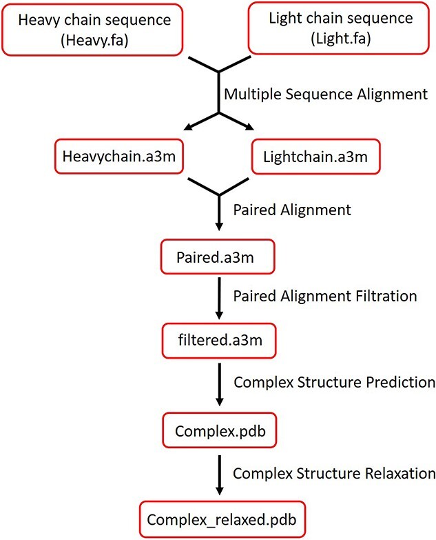
The workflow of modeling with RoseTTAFold. Heavy and light chains sequence is inputted as FASTA files and MSA is performed respectively. Heavy and light chains a3m files were paired by Paired Alignment. After filtering pair alignment results, a complex structure was predicted based on the filtered file. Finally, side chains were added to the model by relaxing the complex.

SWISS-MODEL modeling

To evaluate the performance of RoseTTAFold, we used the webserver of SWISS-MODEL (https://swissmodel.expasy.org/interactive) to predict the structure of the same antibodies as we did with RoseTTAFold. To prepare the inquiry sequence information, we retrieved the heavy and light chains sequences of antibodies from IMGT/3Dstructure-DB and IMGT/2Dstructure-DB Query page (http://www.imgt.org/3Dstructure-DB/). We pasted the heavy/light chain sequence in the Target Sequence work frame (make two independent work frames by using the Add hetero target), then clicked ‘Search for Templates’. We then looked into the raw data (More-Unfiltered Templates as HTML) and selected the template with GMQE score we need as well as a high sequence coverage (at least covering the sequence of six CDR loops). After selecting a model, we utilized Build Monomer to complete the model construction.

ABodyBuilder modeling

For modeling the structures by ABodyBuilder, we chose to use the webserver (http://opig.stats.ox.ac.uk/webapps/newsabdab/sabpred/abodybuilder/) on SAbPred’s website. First, we uploaded the sequences of heavy and light chains of antibodies into the system, and the MODELLER was selected as the ab initio modeling method if it was required. The annotation of the output structure followed the IMGT numbering scheme. To search the blacklist PDB, we used the sequence searching function in SAbDab. First, we entered the sequence of target antibodies, set the minimum sequence identity as 50% and retrieved 50 structures. To approach the blind prediction, we put the PDB structure whose sequence identity is higher than 90% in the blacklist and subsequently excluded them during the template searching. The best model in the outputs was used as the final model.

RMSD calculation

The root mean square deviation (RMSD) for model assessment was calculated over the backbone atoms (N, CA, C, O). The RMSDs of the CDR regions were computed after superposing the corresponding framework regions (FRs). For example, when we compared the CDR H1–H3, the model framework region of the heavy chain (FRH) was superposed onto the crystal FRH, then we calculated the RMSD of CDR H1–H3. The comparisons of CDR regions were computed by the McLachlan fitting algorithm [30], which is within the ProFit software [31]. The comparisons of the whole structures were computed by a fitting function of PyMOL.

Statistical analysis

The original data were transformed to logarithms and was calculated the means of each group by using Descriptive statistics. Because the one-way analysis of variance (ANOVA) test requires data to be normally distributed and have the same variance, we found that some groups of our data did not fit the requirements of one-way ANOVA. To ensure the accuracy of data analysis, we first applied statistical methods to verify if our data were normally distributed and had the same variance. According to the verification results, we chose the most suitable methods to test the significant differences between the means of each group. Normal distribution of the data was tested by the D’Agostino-Pearson normality test, and differences in standard deviation among groups with normally distributed data were tested by Bartlett’s and Brown–Forsythe tests. Statistical analyses in multiple groups with normally distributed data and no significant differences in standard deviation were then compared with the RoseTTAFold group. An ANOVA test was applied to test the means difference between each group and RoseTTAFold, whereas Dunnet’s multiple comparisons test was used to correct for multiple comparisons. When multiple groups with normally distributed data and significant differences in standard deviation were compared with the RoseTTAFold group, we used a Brown–Forsythe and Welch ANOVA and a Dunnet’s multiple comparisons test to evaluate means difference among multiple groups. If multiple groups without normally distributed data were compared with the RoseTTAFold group, a Kruskal–Wallis and a Dunn’s multiple comparisons test were used for post hoc analysis to correct for multiple comparisons. GraphPad Prism 9.0.0 was applied to conduct all statistical analyses.

Results and discussion

We created an antibody test set by collecting 30 antibodies from SAbDab, and all these antibodies have crystal structures. First, RoseTTAFold was used to model all the antibodies by applying the ‘predicting complex structure’ method provided by RoseTTAFold on GitHub.

SWISS-MODEL predicts antibody structures based on GMQE score with three different ranges

To evaluate the quality of structures predicted by RoseTTAFold equal to the modeled structures based on what ranges of GMQE score, the modeled structures of SWISS-MODEL were stratified into three different ranges, including [0.9–0.8), [0.8–0.7) and [0.7–0.6). Briefly, the GMQE score is one of the key metrics used to measure the quality of a template, which predicts the Local Distance Difference Test score of the resulting model. GMQE score includes all of the properties of the target-template alignment (including sequence similarity, sequence identity, agreement of the predicted secondary structure between target and template, HHblits score, agreement between predicted solvent accessibility between target and template) and normalizes them based on alignment length, then combines them. GMQE gives an overall model quality measurement between 0 and 1 by higher numbers indicating higher expected quality. Compared with other metrics in SWISS-MODEL, GMQE is one of the main metrics and it has a positive correlation with 3D models’ quality. The change of GMQE score more directly reflects the quality of models, which is more suitable for evaluating the quality of structures predicted by RoseTTAFold. The test set antibodies were modeled three times, and each time, the templates were selected from different GMQE ranges. Due to the limited results produced by SWISS-MODEL, we just found templates with GMQE ranging from 0.7 to 0.6 for 12 antibodies in the test set. Because the fluctuation of the residue side chains is not representative of overall conformational change, backbone atoms are more suitable to investigate large-scale movements in proteins. Therefore, after all the structures were modeled, we used ProFit to calculate the backbone RMSDs of six CDR domains between the structures modeled by SWISS-MODEL and the crystal structures. Then we calculated and compared the average RMSDs of structures modeled by RoseTTAFold and those of SWISS-MODEL through GraphPad.

RoseTTAFold predicts antibody models with acceptable quality

Figure 2 compares the RMSDs of six CDR loops, and Supplementary Table S2 shows the original data before logarithm transformation. First, we observed that the RMSD of the H3 loop was higher than other CDR loops in the two methods, whereas L2 had the lowest RMSD among the others (comparing Figures 2A–F). These results indicated that the predicted H3 loop was not as good as its crystal structure, but the predicted L2 loop was close to its crystal structure. These findings proved that the H3 loop is the most difficult part to be modeled due to its variability, whereas L2 is the easiest one to be modeled among the six CDR loops. Except for the H3 loop (the average RMSD approximates 3 Å), the average RMSDs of the other five CDR loops modeled by RoseTTAFold were lower than 2 Å, indicating that structures produced by RoseTTAFold were of acceptable quality (Figure 2A, B, D, E and F).

Figure 2.

Comparing RoseTTAFold with SWISS-MODEL through RMSDs of six CDR loops. Red boxes represent structures that chose templates with a GMQE score ranging from 0.9 to 0.8. Orange boxes represent structures that chose templates with a GMQE score ranging from 0.8 to 0.7. Yellow boxes represent GMQE scores ranging from 0.7 to 0.6. Pink boxes are structures modeled by RoseTTAFold. All RMSDs are reported in logarithmic format. Data of figures A, C and F were analyzed with the Kruskal–Wallis test and Dunn’s multiple comparison test. Data of figures B, D and E were analyzed with the Brown–Forsythe and Welch ANOVA test (^*P < 0.05, ^**P < 0.01 and ^***P < 0.001). Data are present as mean ± standard deviation. The top, center, bottom of the boxplot represent maximum, mean, minimum, respectively.

RoseTTAFold has the same performance with the structures used template with GMQE score ranging from 0.8 to 0.7

For H1, H2, L1 and L3 loops, especially H2, L1, and L3 loops which have high contact frequency with antigens [32], the quality of their structures modeled by RoseTTAFold had no significant difference with the structures of SWISS-MODEL in the group where GMQE score of the template(s) ranged from 0.6 to 0.8. But their quality was not as good as the structures with the template(s) whose GMQE score ranged from 0.8 to 0.9 (Figure 2A, B, D and F). For the models of H3 and L2 loops, 3D structures generated by RoseTTAFold showed a significant difference to the structures by templates with a GMQE score ranging from 0.7 to 0.9. The structures modeled by RoseTTAFold outperformed structures with the template(s) whose GMQE score ranged from 0.6 to 0.7 but showed worse performance than structures with the template(s) whose GMQE score higher than 0.7 (Figure 2C and E). The RMSDs of structures modeled by SWISS-MODEL increased along with the increased GMQE score of templates, which was consistent with the fact that the lower similarity of the template it chose, the worse quality of the model it would be (comparing Figure 2A–F). Here, we chose one antibody as an example to show the structural differences modeled by either RoseTTAFold or SWISS-MODEL. Figure 3 shows the structural comparison of the antibody ch28/11 Fab (PDB: 6UGA): the pink model is the structure modeled by RoseTTAFold, the structure highlighted in green is modeled by SWISS-MODEL (GMQE score: 0.8–0.9) and the white one is the crystal structure. The RMSDs of six CDR loops modeled by SWISS-MODEL/RoseTTAFold were H1: 1.430/1.418, H2: 1.199/1.519, H3: 1.705/1.306, L1: 1.141/1.026, L2: 0.261/0.880, L3: 0.472/1.746 (unit: Å). The results indicated that for structure modeled by templates with a GMQE score higher than 0.8, the RMSDs of CDR loops modeled by SWISS-MODEL were lower than those modeled by RoseTTAFold. All these data supported that for most of the CDR loops modeling, RoseTTAFold could model structures with similar quality with SWISS-MODEL when the GMQE score of the template(s) is lower than 0.8.

Figure 3.

Comparing RoseTTAFold with structures modeled by templates with GMQE score 0.8–0.9. The yellow regions represent the six CDR loops. The crystal structure was retrieved from PDB:6UGA. All RMSDs are reported in Å.

The quality of structures modeled by RoseTTAFold is equal to the structures used template with GMQE score ranging from 0.8 to 0.7 in longitudinal comparison

To validate the reliability of our finding, we randomly chose six antibodies from the list and modeled them by RoseTTAFold and SWISS-MODEL. SWISS-MODEL was applied to model each of them three times, in which we selected templates with different ranges of GMQE per time. When comparing the results modeled by RoseTTAFold with that of SWISS-MODEL, we noticed that the RMSDs of models constructed by SWISS-MODEL decreased along with the increased GMQE score of the template. Taking the antibody HFE7A (PDB: 1IT9) as an example, its RMSDs (Å) of H1, H2, H3, L1 and L3 loops increased gradually (from 0.508 to 3.127, 0.521 to 1.172, 2.693 to 5.221, 1.383 to 2.540 and 1.165 to 1.694, respectively) when the GMQE score decreased from 0.9 to 0.6 (Figure 4 and Table 1). Table 2 shows the RMSDs result of six antibodies, and we observed that for most of the CDR loops modeled by RoseTTAFold, their RMSDs were close to the structures modeled by templates with a GMQE ranging from 0.6 to 0.8, but were higher than structures modeled by templates with a GMQE from 0.8 to 0.9. In summary, when the GMQE score of templates was higher than 0.8, SWISS-MODEL performed better than RoseTTAFold. Otherwise, RoseTTAFold modeled antibodies with high accuracy.

Figure 4.

Comparison of 3D structures modeled by RoseTTAFold and modeled by SWISS-MODEL with different GMQE scores. The green structure was modeled by templates with GMQE scores from 0.7 to 0.6; the cyan structure was modeled by templates with GMQE scores from 0.8 to 0.7; the pink structure was modeled by templates with GMQE scores from 0.9 to 0.8. The yellow regions represent the six CDR regions. The crystal structure was generated from the antibody HFE7A (PDB: 1IT9).

Table 1.

RMSDs of six CDR loops of the antibody HFE7A modeled by three templates with different GMQE scores

Variable region Range of GMQE	H1	H2	H3	L1	L2	L3
(0.8–0.9]	0.508	0.521	2.693	1.383	0.536	1.165
(0.7–0.8]	1.166	0.594	4.213	1.859	0.873	1.234
(0.6–0.7]	3.127	1.172	5.221	2.540	0.788	1.694

All RMSDs are reported in Å.

Table 2.

RMSDs of six antibodies’ CDR loops modeled by RoseTTAFold and SWISS-MODEL with different GMQE score templates

PDB	Methods	H1	H2	H3	L1	L2	L3
1IT9	RF	1.271	1.464	4.279	3.306	0.975	1.958
	SM1	0.508	0.521	2.693	1.383	0.536	1.165
	SM2	1.166	0.594	4.213	1.859	0.873	1.234
	SM3	3.127	1.172	5.221	2.540	0.788	1.694
4R4B	RF	1.149	3.314	1.934	1.570	1.195	2.372
	SM1	1.497	3.476	2.260	1.070	0.351	1.127
	SM2	1.194	3.029	2.243	1.591	1.060	1.612
	SM3	5.442	3.685	6.179	0.909	0.666	1.454
5F6H	RF	1.602	0.950	1.536	2.366	2.110	2.481
	SM1	2.250	1.294	1.356	0.725	1.076	1.582
	SM2	0.851	1.683	2.593	1.007	1.353	2.185
	SM3	2.132	2.747	2.958	1.853	1.654	1.426
5YSL	RF	1.844	3.177	0.998	0.614	1.272	1.198
	SM1	1.490	1.553	3.134	1.811	0.990	2.102
	SM2	4.678	1.266	2.688	5.345	0.502	1.103
	SM3	2.907	3.528	3.668	1.455	0.580	0.882
6PZH	RF	2.425	1.182	4.280	2.001	2.619	1.987
	SM1	0.605	0.652	1.979	0.579	1.146	0.830
	SM2	0.514	1.085	5.985	3.499	0.368	2.967
	SM3	2.918	3.693	9.206	1.542	2.014	2.359
6VU2	RF	2.320	2.133	5.187	2.672	1.922	1.987
	SM1	0.097	0.093	1.106	0.115	0.128	0.082
	SM2	2.230	3.025	5.629	4.692	0.677	2.433
	SM3	3.273	2.803	5.160	4.608	1.385	2.417

RF means RoseTTAFold. SM¹: SWISS-MODEL with GMQE from (0.8 to 0.9]; SM²: SWISS-MODEL with GMQE from (0.7 to 0.8]; SM³: SWISS-MODEL with GMQE from (0.6 to 0.7]. All RMSDs are reported in Å.

The quality of structures modeled by RoseTTAFold still have a gap with those of structures modeled by SWISS-MODEL and ABodyBuilder

To further compare RoseTTAFold with other antibody modeling software, we compared RoseTTAFold with SWISS-MODEL (homology modeling-based) and ABodyBuilder (antibody specialized homology modeling) to assess the ability of antibody modeling of RoseTTAFold. To approach blind prediction, we excluded templates with a sequence identity over 90% for both SWISS-MODEL and ABodyBuilder. To improve the accuracy of structures predicted by SWISS-MODEL, we referred to the GMQE score to search the templates of each target antibody. After modeling by ABodyBuilder, we used ProFit to calculate the backbone RMSDs between the crystal structures and the modeled ones. Then, we applied GraphPad to calculate the average RMSDs of three methods. Supplementary Figure S1 shows the average RMSD of the whole antibody modeled by RoseTTAFold has a significant difference with SWISS-MODEL and ABodyBuilder. Supplementary Table S3 shows that the average RMSD of all of the antibody structures modeled by RoseTTAFold was 1.472 Å, which was within the acceptable quality. For SWISS-MODEL and ABodyBuilder, their RMSDs were 0.947 Å and 0.943 Å, respectively. Because the quality of the CDR domains is the most important metric for evaluating the performance of antibody modeling, we mainly focused on evaluating the CDR domains.

Figure 5 indicates that apart from the H3 loop, the quality of other CDR loops modeled by RoseTTAFold showed a significant difference with CDR loops modeled by the other two methods. Although RoseTTAFold could accurately predict antibody 3D structures, its quality is still not as good as the other two methods (Figure 5A, B, D, E and F, Supplementary Table S4). Unexpectedly, for H3 loop modeling, which is the core challenge for antibody modeling, the RMSD of the H3 loop modeled by RoseTTAFold did not illustrate a significant difference with the H3 loop modeled by ABodyBuilder and SWISS-MODEL. This result suggested that in H3 loop modeling, the accuracy predicted by RoseTTAFold was comparable to ABodyBuilder and SWISS-MODEL.

Figure 5.

Evaluation of three methods by comparing RMSDs of six CDR loops. (A) RMSD of H1 loop; (B) RMSD of H2; (C) RMSD of H3; (D) RMSD of L1; (E) RMSD of L2; (F) RMSD of L3. The model FR was superposed onto the corresponding crystallographic framework before computing the RMSDs of CDR loops. All RMSDs are reported in logarithmic format. Data of figures A, B, C and D were analyzed with the Brown–Forsythe and Welch ANOVA test. Data of figures E and F were analyzed with the one-way ANOVA test and an additional Dunnet’s multiple comparisons test (^*P < 0.05, ^**P < 0.01 and ^***P < 0.001). Data are presented as mean ± standard deviation. The top, center and bottom of the boxplot indicate maximum, mean, minimum, respectively. RF: RoseTTAFold; SM: SWISS-MODEL; AB: ABodyBuilder.

RoseTTAFold can model H3 loop more accurate than ABodyBuilder

Although the backbone RMSD between modeled structure and crystal structure was small, sometimes the modeling methods may not accurately model the secondary structure of the loops (Figure 6A and B, and Supplementary Figure S2). For example, in Figure 6B, despite the RMSD of the antibody 1H1 (PDB: 5YSL) H3 loop modeled by SWISS-MODEL was the smallest among the three methods, SWISS-MODEL did not form the beta sheet as the crystal structure, which indicated an incorrect prediction in the modeling. However, RoseTTAFold showed the ability to model that beta sheet of the H3 loop correctly. On the contrary, in the H1 loop of the antibody EP2-19G2 (PDB:3CFC) (Figure 6A), RoseTTAFold failed in modeling the helix on the structure. But SWISS-MODEL and ABodyBuilder could successfully model that of the helix. We defined the modeled structures which did not form a correct secondary structure as failure modeling. We then summed the total numbers of failure modeling in each CDR domain predicted by three methods. From Table 3, we can see that although the L2 loop is the easiest loop to be modeled, its failure numbers were not very low. On the contrary, the L3 loop had the lowest failure modeling numbers. H3 and H1 had the highest failure rates among the three methods. Based on the observation, we found that for H1 loop modeling, RoseTTAFold always failed to model the helix on the H1 loop. Although there was no statistically significant difference among the three methods for H3 modeling, the failure modeling numbers of secondary-structure of RoseTTAFold were lower than ABodyBuilder and close to SWISS-MODEL. All these results suggest that RoseTTAFold could predict the H3 loop more accurately than ABodyBuilder, but for the rest of the loops modeling, there were still some gaps when compared with the other two methods.

Figure 6.

RMSD of 3CFC H1 loop and 5YSL H3 loop modeled by three methods. (A) 3CFC H1 loop modeled by three methods. RMSDs for ABodyBuilder, RoseTTAFold and SWISS-MODEL are 2.003, 1.888 and 2.506 Å, respectively. (B) 5YSL H3 loop modeled by three methods. RMSDs for ABodyBuilder, RoseTTAFold and SWISS-MODEL are 2.519, 3.134 and 2.415 Å, respectively.

Table 3.

Failure modeling numbers of six CDR loops for the three methods

Variable Region Methods	H1	H2	H3	L1	L2	L3
RoseTTAFold	16	7	8	6	3	5
SWISS-MODEL	7	3	9	8	9	1
ABodyBuilder	9	3	12	3	8	1

Numbers are summed from six CDR loops of 30 antibodies.

Limitations and future improvement

Assessing the performance of three methods, RoseTTAFold could predict the antibody structures lower than 2 Å, but its accuracy still had a definitive gap with SWISS-MODEL. Due to the limited number of templates, the result of 0.6–0.7 may be biased when compared with other groups with different GMQE scores. Currently, RoseTTAFold is trained only on monomeric proteins, rather than complexes. This results in RoseTTAFold being less capable of predicting complexes than monomeric proteins. In addition, RoseTTAFold currently employs the databases UniRef30 (a 30% sequence identity-clustered database based on Uniprot Reference Clusters knowledgebase) and big fantastic database (BFD) (created by clustering protein sequences from Uniprot/TrEMBL+Swissprot) which do not include many antibody sequences and limit the extraction of residue-residue coevolution information. The other challenge is that there is still a limited number of antibody sequences available for network learning, which affects the accuracy of antibody modeling. Recently, RoseTTAFold mainly focused on modeling the interaction between the complexes, but the CDR regions in antibodies have unique structures and require additional consideration. The reason why RoseTTAFold has a higher failure rate in modeling helix in the H1 loop maybe that RoseTTAFold uses the end-to-end three-track network to model complex structures. Due to the negligence of side chain information and the limitations of computational memory, the end-to-end version cannot fully improve the structure and needs the optimization of FastRelax, which may cause a certain number of secondary structure modeling failures. Although there are still some limitations for RoseTTAFold, in most cases of the engineered antibodies that do not have 3D structures, they can find a template with a GMQE score range from 0.7 to 0.8. For some new antibodies, there may not be a template with a GMQE score higher than 0.5. The paper generated results that indicate RoseTTAFold could have similar performance with the structures when the GMQE score of their templates is lower than 0.8. This is true especially for the high frequency of antigen contact loops H1, H2 and L3. RoseTTAFold can model H3 loop more accurate than ABodyBuilder. These results illustrate the usability of RoseTTAFold in antibody modeling. At the same time, they give insight into the potential that RoseTTAFold can outperform traditional methods, especially when there are no homologous structures available. In the future, the protein–protein complexes datasets can be applied to train the network of RoseTTAFold. It can also include the database which specifies antibodies, such as IMGT and SAbDab, which will facilitate the MSA process and extract the coevolution information more easily. Trained with antibody-specifies databases, the interresidue distances and orientations can be predicted more accurate, improving the accuracy of secondary structure prediction, for example, H1 loop modeling. An alternative method to increase the accuracy of secondary structure prediction is to use pyRosetta to model complex instead of the end-to-end version. PyRosetta incorporates side chain information at the all-atom relaxation stage, which can precisely predict secondary structure. Therefore, it is a good idea to modify the code of pyRosetta and apply it to model complex structures. To increase the accuracy of CDR loops modeling, it might need to incorporate some physical theories and parameters or have extra training.

Conclusion

In antibody modeling, RoseTTAFold can predict antibody structures with acceptable quality without the training by complex proteins datasets. Evaluating the performance between RoseTTAFold and SWISS-MDOEL, RoseTTAFold could achieve similar performance to SWISS-MODEL when the template structures with GMQE score lower than 0.8. In further comparison between RoseTTAFold and the homology modeling-based methods SWISS-MODEL and ABodyBuilder, RoseTTAFold still showed a conclusive gap with them. Although for H1 region modeling, RoseTTAFold always failed to model the helix on it, it could predict H3 loop more accurately than ABodyBuilder and comparable to SWISS-MODEL. These results indicate that RoseTTAFold could achieve higher accuracy in antibody modeling, and with further improvement of the algorithm, it can rapidly generate atomic accuracy antibody structures.

Key Points

• RoseTTAFold can predict antibody 3D structures accurately without the training by complex proteins datasets. For the CDR loops modeling, excluding the H3 loop, it can predict structures with RMSDs lower than 2 Å.

• There is no statistically significant difference between the quality of the H3 loop modeled by RoseTTAFold, SWISS-MODEL and ABodyBuilder. RoseTTAFold had higher success rates in predicting secondary structures of the H3 loop than ABodyBuilder. RoseTTAFold can predict the H3 loop with more accuracy than ABodyBuilder and is comparable to SWISS-MODEL.

• RoseTTAFold can achieve similar accuracy in predicting antibody structures to SWISS-MODEL when structures with templates whose GMQE is lower than 0.8 are used. It shows the potential of RoseTTAFold’s antibody modeling to outperform traditional methods, especially when there are no homologous structures for a target antibody.

Tianjian Liang is currently a first-year PhD student in the School of Pharmacy, University of Pittsburgh. His research interests are antibody-drug design and systems pharmacology analysis.

Chen Jiang is currently a second-year master student in the School of Pharmacy, University of Pittsburgh. Her research interests are GPCR drug design and clinical pharmacy.

Jiayi Yuan is a second-year master student in the School of Pharmacy, University of Pittsburgh. Her research interest is computer-aided drug design, which includes CB2 allosteric modulators as well as antigen/antibody design.

Yasmin Othman is currently a first-year undergraduate student in the School of Engineering at Penn State University. She is a research volunteer in Professor Zhiwei Feng’s lab.

Xiang-Qun Xie received his PhD degree in 1993 from the University of Connecticut. He is an Associate Dean of PharmacoAnalytics and Professor of an integrated Medicinal Chemistry Biology Platform of Computational Lab, Biology Lab, and Chemical Lab at the University of Pittsburgh School of Pharmacy. He serves as a Charter Member of the US FDA Science Advisory Board.

Zhiwei Feng got his PhD degree from Soochow University in 2013. He is currently an assistant professor in the School of Pharmacy, University of Pittsburgh. His research interests include (i) the development of algorithms/tools/apps for drug discovery, (ii) chemogenomic knowledgebase design and novel tool development for drug design of small molecules and modulators (iii) and big-data or clinical data analysis and pharmacometrics and systems pharmacology.

Authors’ Contributions

Z.F. and X.-Q. X. designed the project. T.L. and C.J. tested the code, prepared the figures, and wrote the manuscript. All authors read and approved the final manuscript.

Funding

The authors would like to acknowledge the funding support to the Xie laboratory/Center from the NIH NIDA NIH NIDA (R01DA052329 and P30 DA035778A1).

Conflict of Interest

The authors declare that they have no competing interests.

Availability

The RoseTTAFold is accessible from https://github.com/RosettaCommons/RoseTTAFold. All the data presented in this work can be found in https://github.com/stcmz/antibody-modelling-benchmark.

References

- 1. Janeway CA. Immunobiology: The Immune System in Health and Disease. New York: Garland Science, 2001. [Google Scholar]
- 2. Weitzner BD, Kuroda D, Marze N, et al. Blind prediction performance of Rosetta antibody 3.0: grafting, relaxation, kinematic loop modeling, and full CDR optimization. Proteins 2014;82:1611–23. [DOI] [PMC free article] [PubMed] [Google Scholar]
- 3. Lu R-M, Hwang Y-C, Liu IJ, et al. Development of therapeutic antibodies for the treatment of diseases. J Biomed Sci 2020;27(1):1. [DOI] [PMC free article] [PubMed] [Google Scholar]
- 4. Shen X, Kosten TR. Immunotherapy for drug abuse, CNS & neurological disorders drug targets. CNS Neurol Disord Drug Targets 2011;10:876–9. [DOI] [PMC free article] [PubMed] [Google Scholar]
- 5. Chen J, Gao K, Wang R, et al. Review of COVID-19 antibody therapies. Annu Rev Biophys 2021;50:1–30. [DOI] [PMC free article] [PubMed] [Google Scholar]
- 6. Marcatili P, Olimpieri PP, Chailyan A, et al. Antibody modeling using the prediction of Immuno globulin structure (PIGS) web server. Nat Protoc 2014;9:2771–83. [DOI] [PubMed] [Google Scholar]
- 7. Wang X, Li F, Qiu W, et al. SYNBIP: synthetic binding proteins for research, diagnosis and therapy. Nucleic Acids Res 2022;50:D560–70. [DOI] [PMC free article] [PubMed] [Google Scholar]
- 8. Marsh JA, Teichmann SA. Structure, dynamics, assembly, and evolution of protein complexes. Annu Rev Biochem 2015;84:551–75. [DOI] [PubMed] [Google Scholar]
- 9. Chothia C, Lesk AM. Canonical structures for the hypervariable regions of immunoglobulins. J Mol Biol 1987;196:901–17. [DOI] [PubMed] [Google Scholar]
- 10. Waterhouse A, Bertoni M, Bienert S, et al. SWISS-MODEL: homology modelling of protein structures and complexes. Nucleic Acids Res 2018;46:W296–w303. [DOI] [PMC free article] [PubMed] [Google Scholar]
- 11. Hatherley R, Brown DK, Glenister M, et al. PRIMO: an interactive homology Modeling pipeline. PLoS One 2016;11:e0166698-e0166698. [DOI] [PMC free article] [PubMed] [Google Scholar]
- 12. Webb B, Sali A. Comparative protein structure Modeling using MODELLER. Curr Protoc Bioinformatics 2016;54:5.6.1–37. [DOI] [PMC free article] [PubMed] [Google Scholar]
- 13. Cavasotto CN, Phatak SS. Homology modeling in drug discovery: current trends and applications. Drug Discov Today 2009;14:676–83. [DOI] [PubMed] [Google Scholar]
- 14. Sivasubramanian A, Sircar A, Chaudhury S, et al. Toward high-resolution homology modeling of antibody Fv regions and application to antibody-antigen docking. Proteins 2009;74:497–514. [DOI] [PMC free article] [PubMed] [Google Scholar]
- 15. Leem J, Dunbar J, Georges G, et al. ABodyBuilder: automated antibody structure prediction with data-driven accuracy estimation. MAbs 2016;8:1259–68. [DOI] [PMC free article] [PubMed] [Google Scholar]
- 16. Marcatili P, Rosi A, Tramontano A. PIGS: automatic prediction of antibody structures. Bioinformatics 2008;24:1953–4. [DOI] [PubMed] [Google Scholar]
- 17. Zhu K, Day T, Warshaviak D, et al. Antibody structure determination using a combination of homology modeling, energy-based refinement, and loop prediction. Proteins 2014;82:1646–55. [DOI] [PMC free article] [PubMed] [Google Scholar]
- 18. Almagro JC, Beavers MP, Hernandez-Guzman F, et al. Antibody modeling assessment. Proteins 2011;79:3050–66. [DOI] [PubMed] [Google Scholar]
- 19. Bujotzek A, Dunbar J, Lipsmeier F, et al. Prediction of VH-VL domain orientation for antibody variable domain modeling. Proteins 2015;83:681–95. [DOI] [PubMed] [Google Scholar]
- 20. Jumper J, Evans R, Pritzel A, et al. Highly accurate protein structure prediction with AlphaFold. Nature 2021;596:583–9. [DOI] [PMC free article] [PubMed] [Google Scholar]
- 21. Kryshtafovych A, Schwede T, Topf M, et al. Critical assessment of methods of protein structure prediction (CASP)—round XIV. Proteins 2021;89:1607–17. [DOI] [PMC free article] [PubMed] [Google Scholar]
- 22. Baek M, DiMaio F, Anishchenko I, et al. Accurate prediction of protein structures and interactions using a three-track neural network. Science 2021;373:871–6. [DOI] [PMC free article] [PubMed] [Google Scholar]
- 23. Lefranc M-P. Complementarity determining region (CDR-IMGT). In: Dubitzky W, Wolkenhauer O, Cho K-Het al. (eds). Encyclopedia of Systems Biology. New York, NY: Springer New York, 2013, 451–3. [Google Scholar]
- 24. Pettersen EF, Goddard TD, Huang CC, et al. UCSF chimera – a visualization system for exploratory research and analysis. J Comput Chem 2004;25:1605–12. [DOI] [PubMed] [Google Scholar]
- 25. Dunbar J, Krawczyk K, Leem J, et al. SAbDab: the structural antibody database. Nucleic Acids Res 2014;42:D1140–6. [DOI] [PMC free article] [PubMed] [Google Scholar]
- 26. Guest JD, Vreven T, Zhou J, et al. An expanded benchmark for antibody-antigen docking and affinity prediction reveals insights into antibody recognition determinants. Structure 2021;29:606–621.e605. [DOI] [PMC free article] [PubMed] [Google Scholar]
- 27. Remmert M, Biegert A, Hauser A, et al. HHblits: lightning-fast iterative protein sequence searching by HMM-HMM alignment. Nat Methods 2012;9:173–5. [DOI] [PubMed] [Google Scholar]
- 28. Steinegger M, Meier M, Mirdita M, et al. HH-suite3 for fast remote homology detection and deep protein annotation. BMC Bioinformatics 2019;20:473. [DOI] [PMC free article] [PubMed] [Google Scholar]
- 29. Conway P, Tyka MD, DiMaio F, et al. Relaxation of backbone bond geometry improves protein energy landscape modeling. Protein Sci 2014;23:47–55. [DOI] [PMC free article] [PubMed] [Google Scholar]
- 30. McLachlan AD. Rapid comparison of protein structures. Acta Crystallogr 1982;38:871–3. [Google Scholar]
- 31. Martin ACR. ProFit. http://www.bioinf.org.uk/software/profit/ (Accessed date: 19 April 2022).
- 32. Akbar R, Robert PA, Pavlović M, et al. A compact vocabulary of paratope-epitope interactions enables predictability of antibody-antigen binding. Cell Rep 2021;34:108856. [DOI] [PubMed] [Google Scholar]
Associated Data
This section collects any data citations, data availability statements, or supplementary materials included in this article.