Bayesian modeling of spatial molecular profiling data via Gaussian process

Abstract

Motivation

The location, timing and abundance of gene expression (both mRNA and proteins) within a tissue define the molecular mechanisms of cell functions. Recent technology breakthroughs in spatial molecular profiling, including imaging-based technologies and sequencing-based technologies, have enabled the comprehensive molecular characterization of single cells while preserving their spatial and morphological contexts. This new bioinformatics scenario calls for effective and robust computational methods to identify genes with spatial patterns.

Results

We represent a novel Bayesian hierarchical model to analyze spatial transcriptomics data, with several unique characteristics. It models the zero-inflated and over-dispersed counts by deploying a zero-inflated negative binomial model that greatly increases model stability and robustness. Besides, the Bayesian inference framework allows us to borrow strength in parameter estimation in a de novo fashion. As a result, the proposed model shows competitive performances in accuracy and robustness over existing methods in both simulation studies and two real data applications.

Availability and implementation

The related R/C++ source code is available at https://github.com/Minzhe/BOOST-GP.

Supplementary information

Supplementary data are available at Bioinformatics online.

1 Introduction

Investigating the spatial organization of cells, together with their mRNA and protein abundances, is essential to delineating how cells from different origins form tissues with distinctive structures and functions. Traditional molecular profiling technologies require tissue-dissociation, which leads to the loss of the spatial context of gene expression, while traditional imaging technologies can only measure the levels of several markers. Thus, the spatial information of tissues and the high-throughput molecular profile, for a long time, were analyzed individually with little crosstalk.

Recent technology breakthroughs in spatial molecular profiling (SMP) empower the comprehensive molecular characterization at a high spatial resolution. There are two major types of SMP techniques: imaging-based methods based on the single-molecule fluorescence in situ hybridization (FISH), such as sequential FISH (seqFISH) (Eng et al., 2019; Lubeck et al., 2014) and multiplexed error-robust FISH (MERFISH) (Chen et al., 2015), and sequencing-based methods, such as spatial transcriptomics sequencing (STS) (Ståhl et al., 2016) and slide-sequencing (Rodriques et al., 2019). The overview of their workflows is shown in Figure 1a. We could view the imaging-orientated approaches as regular FISH imaging integrated with multi-round re-hybridization, which allows multiplexing. The sequencing-orientated approaches can be regarded as traditional sequencing technology with additional spatial barcoding to restore spatial information. We recently published a review paper to discuss technical details on SMP platforms (Zhang et al., 2021). In all, these SMP technologies combine the spatial information of tissues and the high-throughput molecular profile, enabling mapping and measuring the gene expression of thousands of cells over a tissue slide simultaneously.

Fig. 1.

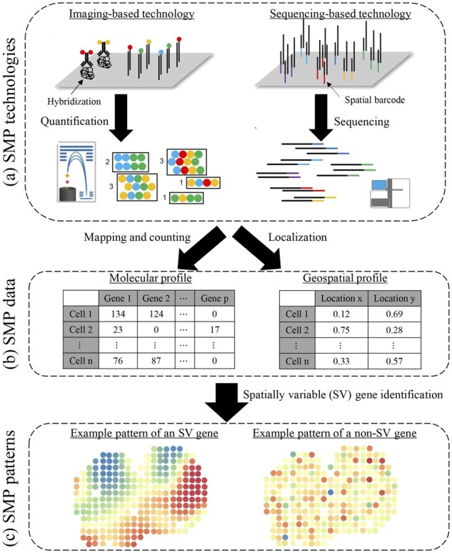
Flowchart of an SMP study. (a) Hybridization and quantification phases in imaging-based SMP technologies (left) and barcoding and sequencing phases in sequencing-based SMP technologies (right). (b) An example of molecular profile Y (left) and an example of geospatial profile T (right). (c) Examples of molecular spatial distributions to an SV gene and a non-SV gene

Many new questions can be studied with this powerful new technology available. One of the most immediate ones is to identify genes whose expressions display spatially correlated patterns, which we refer to as spatially variable (SV) genes (see an example in Fig. 1c). Such genes may reflect the tissue heterogeneity and underlying tissue structure that drive the differentiated expression across different spatial locations. Thus, they are potentially significant and may lead to new biological insights. Statistically, identifying SV genes is a new challenge to test the association between gene-expression levels and their spatial coordinates with a null hypothesis of spatial invariance. Several methodologies have been recently proposed for this task. SpatialDE (Svensson et al., 2018) and SPARK (Sun et al., 2020) are two that adopt a Gaussian process (GP), which serves as a natural fit for this problem because of its ability to model temporal (Roberts et al., 2013) or spatial (Diggle et al., 1998) dependence via a pre-specified kernel. They share the same geostatistical modeling framework, with SPARK being more explicit in modeling count data, sample normalization and P-value calibration. Trendsceek (Edsgärd et al., 2018) is another method that models the spatial gene expression of cells as a realization marked point process. Its idea is to calculate several summary statistics for all pairwise points with respect to their distances and evaluate the significance under null distribution generated with random permutations.

All of these methods are for identifying SV genes in SMP data, while still leaving several issues unsolved. First, SpatialDE and Trendsceek transformed count data, which do not truly reflect the underlying data generative mechanism. Although SPARK used a Poisson distribution for modeling counts, the simple mean-variance relationship may not be sufficient in accounting for the over-dispersion observed in real sequencing data. Second, typical SMP data contain a large proportion of zero counts (e.g. 60–99%), and none of the mentioned methods properly addressed the zero count, which may largely reduce the statistical power. Table 1 shows a brief summary of four widely analyzed SMP cohorts. Last but not least, SpatialDE and SPARK both employ GP to estimate spatial covariance but only at certain predefined length-scales of the spatial kernels, which means the estimation is only an approximated solution.

Table 1.

A summary of four widely analyzed SMP cohort data

Name	Technique	No. of datasets	No. of dimensions K	No. of locations n	No. of genes p	zero prop. (%)	Reference
Mouse olfactory bulb (MOB)	STS	12 replicates	2	231–282 spots	15 284–16 675	89–90	Ståhl et al. (2016)
Human breast cancer (BC)	STS	4 layers	2	251–264 spots	14 789–14 929	60–79	Ståhl et al. (2016)
Mouse hypothalamus	MERFISH	31 individuals	2	4877–6000 cells	160–161	59–68	Moffitt et al. (2018)
Mouse hippocampus	seqFISH	21 fields	3	97–362 cells	249	1–18	Shah et al. (2016)

Note: STS, spatial transcriptomics sequencing; MERFISH, multiplexed error-robust fluorescence in situ hybridization; seqFISH, sequential fluorescence in situ hybridization.

To address the issues mentioned above, we developed Bayesian mOdeling Of Spatial Transcriptomics data via Gaussian Process (BOOST-GP), which integrates the GP to capture the spatial correlation. Note that although the name only includes spatial transcriptomics data, the proposed method can be applied to analyze other SMP data without modification. BOOST-GP directly models count data using a negative binomial (NB) distribution, which was also adopted by widely used RNA-seq analysis tools, such as DESeq2 (Love et al., 2014) and edgeR (Robinson et al., 2010) to account for the over-dispersion observed in real sequencing data. Previous studies in single-cell RNA-seq (scRNA-seq) data analysis have shown that accounting for the large proportion of zero counts in the model significantly improves the model fitting and accuracy in identifying differentially expressed genes (Finak et al., 2015; Kharchenko et al., 2014; Lun et al., 2016). One novelty of this study is to explicitly accounts for the excess zeros through a zero-inflated negative binomial (ZINB) model. Furthermore, it uses a Bayesian inference framework to improve parameter estimations and quantify uncertainties. We demonstrated the advantages of BOOST-GP in robust inference across various spatial patterns and minimally affected performance when data contains zero-inflation in the simulation study. We also applied BOOST-GP to two real spatial transcriptomics datasets, and BOOST-GP shows an outstanding sensitivity–specificity balance compared to existing methods.

The rest of this article is arranged as follows. In Section 2, we formulate the probabilistic generative model and explore the parameters structure. In Section 3, we present the schematic procedure and demonstrate the Markov chain Monte Carlo (MCMC) algorithms. In Sections 4 and 5, we evaluate BOOST-GP via both simulated and real data. The last section concludes the article and proposes some potential future work.

2 Model

In this section, we present BOOST-GP for identifying SV genes in SMP data. Supplementary Figure S1 and Table S1 summarize the graphical and hierarchical formulation of the proposed model, respectively.

Before introducing the main components, we summarize the observed data as follows. Let a n-by-p count matrix Y denote the molecular profile generated by a spatially resolved transcriptomics technology based on either a sequencing or imaging-based method. The former can measure tens of thousands of genes on spatial locations consisting of a couple of hundred single cells (i.e. $p\gg n$), while the latter directly identifies a large number of individual cells but is only able to measure hundreds of genes simultaneously (i.e. $p\ll n$). Each entry $y_{ij}\in \mathbb{N},i=1,\dots ,n,j=1,\dots ,p$ is the read count observed in sample i (with known location) for gene j. We use the notation ${\mathit{y}}_j$ to denote the j-th column of Y, which represents all read counts belonging to the same gene j. Let a n-by-2 matrix T denote the related geospatial profile, where each row ${\mathit{t}}_i=(t_{i1},t_{i2})\in {\mathbb{R}}^2$ gives the coordinates in a compact subset of the 2D Cartesian plane for sample i. Illustration examples of Y and T are provided in Figure 1b.

2.1 Modeling sequence count data via a ZINB model

In addition to over-dispersion, sequence count data suffer from zero-inflation, especially when the sequence depth is not enough. For instance, the real data analyzed in Marioni et al. (2008) and Witten et al. (2010) contain 40–50% zeros of all numerical values. scRNA-seq data usually have a higher proportion of zero read counts, compared with bulk RNA-seq data (e.g. Finak et al., 2015; Kharchenko et al., 2014; Lun et al., 2016). In general, zero-inflation arises for both biological reasons (e.g. subpopulations of cells or transient states where a gene is not expressed) and technique reasons (e.g. dropouts, where a gene is expressed but not detected through sequencing due to limitation of the sampling effort).

Accommodating toward these characteristics, we start by considering a ZINB model to model the read counts,

$$y_{ij}|{\pi }_i,{\lambda }_{ij},{\varphi }_j\hspace{1em}\sim \hspace{1em}{\pi }_i\mathrm{I}(y_{ij}=0)+(1-{\pi }_i)\text{NB}(s_i{\lambda }_{ij},{\varphi }_j),$$ (1)

where we use $\mathrm{I}(·)$ to denote the indicator function and $\text{NB}(\mu ,\varphi ),\mu ,\varphi >0$ to denote a NB distribution with expectation μ and dispersion $1/\varphi$. Here, we constrain one of the two mixture kernels to be degenerate at zero, thereby allowing for zero-inflation. The sample-specific parameter ${\pi }_i\in (0,1)$ can be viewed as the proportion of extra zero (i.e. false zero or structural zero) counts in sample i. With this NB parameterization, the p.m.f. is written as $\frac{\Gamma (y+\varphi )}{y!\Gamma (\varphi )}{\left(\frac{\varphi }{\mu +\varphi }\right)}^{\varphi }{\left(\frac{\mu }{\mu +\varphi }\right)}^y$, with the variance $\text{Var}(Y)=\mu +{\mu }^2/\varphi$, thus allowing for over-dispersion. A small value of $\varphi$ indicates a large variance to mean ratio, while a large value approaching infinity reduces the NB model to a Poisson model with the same mean and variance.

The NB mean is decomposed of two multiplicative effects, the size factor s_i and the normalized expression level λ_ij. The collection $\mathit{s}=(s_1,\dots ,s_n)$ reflects many nuisance effects across samples, including but not limited to (i) reverse transcription efficiency; (ii) amplification and dilution efficiency; and (iii) sequencing depth. Once the global sample-specific effect is accounted for, λ_ij can be interpreted as the normalized expression level of gene j observed at sample i. Note that such a multiplicative characterization of the NB of Poisson mean is typical in both the frequentist (e.g. Cameron and Trivedi, 2013; Li et al., 2012; Witten, 2011) and the Bayesian literature (e.g. Airoldi and Bischof, 2016; Banerjee et al., 2014) to justify latent heterogeneity and extra over-dispersion in multivariate count data. To ensure identifiability between these two classes of parameters, we follow Sun et al. (2020) to set s_i proportional to the summation of the total number of read counts across all genes for sample i, combined with a constraint of ${\prod }_{i=1}^n{s}_i=1$. It results in $s_i=\sum _{j=1}{y}_{ij}/{\prod }_{i=1}^n\sum _{j=1}{y}_{ij}$. If the main interest is in the absolute gene-expression level (Li et al., 2019), s_i’s can be set to 1. Our modeling approach yields a de-noised version of gene-expression data, i.e. λ_ij’s, after characterizing zero-inflation (via π_i’s), over-dispersion (via ${\varphi }_j$’s) and sample heterogeneity (via s_i’s). Note that although we fix the values of s_i’s, it is possible to use a regularizing prior specification (Li et al., 2017) on s_i’s that allows flexible modeling of count data.

We rewrite model (1) by introducing a latent indicator variable η_ij,

$$\begin{array}{cc}{y}_{ij}|{\eta }_{ij},{\lambda }_{ij},{\varphi }_j\hspace{1em}\sim \hfill & \{\begin{array}{c}\begin{array}{cc}0\hfill & \text{if} {\eta }_{ij}=1\hfill \\ \text{NB}(y_{ij};s_i{\lambda }_{ij},{\varphi }_j)\hfill & \text{if} {\eta }_{ij}=0\hfill \end{array}\hfill \end{array}\hfill \\ \hfill {\eta }_{ij}\hspace{1em}\sim & \text{Bern}({\pi }_i).\hfill \end{array}$$ (2)

The independent Bernoulli prior assumption can be further relaxed by formulating a $\text{Be}(a_{\pi },b_{\pi })$ hyperprior on π_i, leading to a beta-Bernoulli prior of η_ij with expectation $a_{\pi }/(a_{\pi }+b_{\pi })$. Setting $a_{\pi }=b_{\pi }=1$ results in a weakly informative prior on π_i. For all dispersion parameters ${\varphi }_j$’s, we assume a gamma distribution, i.e. ${\varphi }_j\sim \text{Ga}(a_{\varphi },b_{\varphi })$. We recommend small values, such as $a_{\varphi }=b_{\varphi }=0.001$, for a weakly informative setting.

2.2 Identifying SV genes via a geostatistical mixture model

We incorporate the covariates and spatial random process into the model construction by specifying a geostatistical model (Gelfand and Schliep, 2016) for the normalized expression level of gene j for sample i,

$$\text{log}\hspace{0.17em}{\lambda }_{ij}\hspace{1em}=\hspace{1em}{\mathit{x}}_i^{\top }{\mathit{\beta }}_j+w_j({\mathit{t}}_i),$$ (3)

where ${\mathit{x}}_i$ is a R-dimensional column vector of covariates that includes a scalar of one for the intercept and R—1 measurable explanatory variables for sample i at location ${\mathit{t}}_i$. These explanatory variables could be cell types, tissue microenvironment, cell-cycle information and other information that might be important to adjust for during the analysis. ${\mathit{\beta }}_j$ is a R-dimensional column vector of coefficients that includes an intercept representing the mean log-expression of gene j across spatial locations. We denote the collection ${(w_j({\mathit{t}}_1),\dots ,w_j({\mathit{t}}_n))}^{\top }$ by ${\mathit{w}}_j(\mathit{T})$ and assume ${\mathit{w}}_j(\mathit{T})$ is a gene-specific zero-mean stationary GP, modeling the spatial correlation pattern among spatial locations through the covariance ${\sigma }_j^2\mathit{K}(\mathit{T})$ in a multivariate normal distribution, where ${\sigma }_j^2$ is a scaling factor and the kernel $\mathit{K}(\mathit{T})$ is a positive definite matrix with each diagonal entry being one and each off-diagonal entry being a function of the relative position (e.g. Euclidean distance) between each pair of locations, $k_{ij}(||{\mathit{t}}_i-{\mathit{t}}_j||)\in [0,1)$.

The choice of an appropriate kernel function is of critical importance in spatial modeling. A comprehensive overview of many covariance functions can be found in Chapter 4 of Williams and Rasmussen (2006). The use of white noise kernel $\mathit{K}=\mathit{I}$ indicates that i.i.d. noise, multiplied by ${\sigma }_j^2$, is added to the mean log-expression of gene j determined by the covariates. Consequently, no spatial correlation w.r.t. underlying gene-expression levels should be observed across the space T. In contrast, a SV gene is the one that displays significant spatial expression pattern, which is usually defined by a squared exponential (SE) kernel (e.g. Sun et al., 2020; Svensson et al., 2018), where $k_{ij}=\text{exp}(-||{\mathit{t}}_i-{\mathit{t}}_j|{|}^2/2l_j^2)$ with the gene-specific characteristic length-scale denoted by l_j. A large value of l_j encourages the underlying expression levels of distant spots or cells become more correlated.

To identify a subset of gene that is SV across locations, we postulate the existence of a latent binary vector $\mathit{\gamma }={({\gamma }_1,\dots ,{\gamma }_p)}^{\top }$, with ${\gamma }_j=1$ if gene j is an SV gene, and ${\gamma }_j=0$ otherwise. Formulating this assumption, we can rewrite model (3),

$$\text{log}\hspace{0.17em}{\mathit{\lambda }}_j|{\gamma }_j,l_j\hspace{1em}\sim \hspace{1em}\{\begin{array}{c}\begin{array}{cc}\text{MVN}(\mathit{X}{\mathit{\beta }}_j,{\sigma }_j^2\mathit{K})\hfill & \text{if} {\gamma }_j=1\hfill \\ \text{MVN}(\mathit{X}{\mathit{\beta }}_j,{\sigma }_j^2\mathit{I})\hfill & \text{if} {\gamma }_j=0\hfill \end{array}\hfill \end{array}.$$ (4)

A common choice for the prior of the binary latent vector $\mathit{\gamma }$ is a product of Bernoulli distributions on each individual component with a common hyperparameter ω, i.e. ${\gamma }_j\sim \text{Bern}(\omega )$. It is equivalent to a binomial prior on the number of SV genes, i.e. $p_{\gamma }={\sum }_{j=1}^p{\gamma }_j\sim \text{Bin}(p,\omega )$. The hyperparameter ω can be elicited as the proportion of genes expected a priori to be SV. This prior assumption can be further relaxed by formulating a $\text{Be}(a_{\omega },b_{\omega })$ hyperprior on ω, which leads to a beta-binomial prior on $p_{\gamma }$ with expectation $p{a}_{\omega }/(a_{\omega }+b_{\omega })$. We impose a constraint of $a_{\omega }+b_{\omega }=2$ for a vague prior of ω (Tadesse et al., 2005).

Taking a conjugate Bayesian approach, we impose a normal prior on each coefficient in ${\mathit{\beta }}_j$ and an inverse-gamma (IG) prior on ${\sigma }_j^2$; i.e. ${\mathit{\beta }}_j|{\sigma }_j^2\sim \text{MVN}(0,h{\sigma }_j^2\mathit{I})$ and ${\sigma }_j^2\sim \text{IG}(a_{\sigma },b_{\sigma })$. This parameterization setting is standard in most Bayesian normal models. It allows for creating a computationally efficient feature selection algorithm by integrating out the GP mean and covariance scaling factor. The integration leads to marginal non-standardized multivariate student’s t-distributions (MVT) on $\text{log}\hspace{0.17em}{\mathit{\lambda }}_j$. Consequently, we can write the collapsed version of model (4)

$$\begin{array}{c}\hspace{0.17em}\text{log}\hspace{0.17em}{\mathit{\lambda }}_j|{\gamma }_j,l_j\hspace{1em}\sim \\ \hspace{1em}\{\begin{array}{c}\begin{array}{c}{\text{MVT}}_{2a_{\sigma }}\left(0,\frac{b_{\sigma }}{a_{\sigma }}{\left({\mathit{K}}^{-1}-{\mathit{K}}^{-1}\mathit{X}{\mathit{G}}^{-1}{\mathit{X}}^{\top }{\mathit{K}}^{-1}\right)}^{-1}\right)\hfill \\ \text{if} {\gamma }_j=1\hfill \\ {\text{MVT}}_{2a_{\sigma }}\left(0,\frac{b_{\sigma }}{a_{\sigma }}{\left(\mathit{I}-\mathit{X}{({\mathit{X}}^{\top }\mathit{X}+\mathit{I}/h)}^{-1}{\mathit{X}}^{\top }\right)}^{-1}\right)\hfill \\ \text{if} {\gamma }_j=0\hfill \end{array}\hfill \end{array},\end{array}$$ (5)

where $\mathit{G}={\mathit{X}}^{\top }{\mathit{K}}^{-1}\mathit{X}+\mathit{I}/h$. To complete the model specification, we choose a uniform prior $l_j\sim \mathrm{U}(a_l,b_l)$. Following Sun et al. (2020), we suggest the value of a_l and b_l set to be $t^{\text{min}}/2$ and $2t^{\text{max}}$, where $t^{\text{min}}$ and $t^{\text{max}}$ are the minimum and maximum value of the non-zero Euclidean distances across all pairs of spatial locations, respectively.

3 Model fitting

3.1 MCMC algorithm

We use the MCMC algorithm to sample from the posterior distribution. We update the false zero indicator η_ij’s using Gibbs sampler and remaining parameters using a Metropolis–Hastings algorithm. We note that this algorithm is sufficient to guarantee ergodicity for our model. See the details in the Supplementary Material.

3.2 Posterior inference

Our primary interest lies in the identification of SV genes via the selection vector $\mathit{\gamma }$. For each gene, the null and alternative hypotheses are ${\mathcal{M}}_0:{\gamma }_j=0$ and ${\mathcal{M}}_1:{\gamma }_j=1$. We could select the model via calculating the Bayes factor (BF) in favor of ${\mathcal{M}}_1$ over ${\mathcal{M}}_0$, which is defined as the ratio of posterior odds to prior odds. The latter equals $a_{\omega }/b_{\omega }$, while the former can be approximated using the MCMC samples $\{{\gamma }_j^{(1)},\dots ,{\gamma }_j^{(U)}\}$, where U denotes the total number of iterations after burn-in. Thus,

$${\text{BF}}_j=\frac{p({\mathcal{M}}_1|·)}{p({\mathcal{M}}_0|·)}/\frac{p({\mathcal{M}}_1)}{p({\mathcal{M}}_0)}\approx \frac{\sum _{u=1}^U{\gamma }_j^{(u)}/U}{\sum _{u=1}^U\left(1-{\gamma }_j^{(u)}\right)/U}/\frac{a_{\omega }}{b_{\omega }}.$$

The larger the ${\text{BF}}_j$, the more likely gene j is an SV gene, integrating over the uncertainty in all model parameters. We suggest choosing the BF threshold based on the scale for interpretation (Kass and Raftery, 1995).

In addition to BF, we could summarize the posterior distribution of $\mathit{\gamma }$ via maximum-a-posteriori estimates,

$${\mathit{\gamma }}^{\text{MAP}}={\text{argmax}}_{\mathit{\gamma }}\prod _{i=1}^n\prod _{j=1}^{p}f(y_{ij}|{\eta }_{ij},{\lambda }_{ij},{\varphi }_j)p(\text{log}\hspace{0.17em}{\mathit{\lambda }}_j|{\gamma }_j^{(u)},l_j)p({\gamma }_j^{(u)}).$$

A more comprehensive summarization of $\mathit{\gamma }$ is based on their marginal posterior probabilities of inclusion (PPI), where ${\text{PPI}}_j={\sum }_{u=1}^U{\gamma }_j^{(u)}/U$. Then, SV genes are selected if their PPIs are greater than a threshold c,

$${\mathit{\gamma }}^{\text{PPI}}={\left(\mathrm{I}({\text{PPI}}_1\ge c),\dots ,\mathrm{I}({\text{PPI}}_p\ge c)\right)}^{\top }.$$

We suggest choosing the threshold that controls for multiplicity (Newton et al., 2004), which guarantees the expected Bayesian false discovery rate (BFDR) to be smaller than a value. The BFDR is calculated as follows,

$$\text{BFDR}(c)=\frac{\sum _{j=1}^p(1-{\text{PPI}}_j)\mathrm{I}(1-{\text{PPI}}_j<c)}{\sum _{j=1}^p\mathrm{I}(1-{\text{PPI}}_j<c)},$$

where $\text{BFDR}(c)$ is the desired significance level.

4 Simulation study

We used simulated data to assess the performance of BOOST-GP and compare it with that of three alternatives, i.e. Trendsceek (Svensson et al., 2018), SpatialDE (Edsgärd et al., 2018) and SPARK (Sun et al., 2020). We also carried out a sensitivity analysis reported in the Supplementary Material.

We followed the data generative schemes originated by Edsgärd et al. (2018) and Sun et al. (2020) based on two artificially generated spatial patterns and two real spatial patterns in mouse olfactory bulb (MOB) and human breast cancer (BC) data. The first two namely spot and linear patterns, which are shown in Figure 2a and b, were on a 16-by16 square lattice (n = 256 spots). The MOB and BC patterns, which are shown in Figure 2c and d, were on n = 260 and 250 spots, respectively. We simulated p = 100 genes, among which 15 were SV genes while the rest were non-SV genes. For gene j at spot i, its latent normalized expression level on a logarithmic scale was the sum of three components, $\text{log}({\lambda }_{ij})={\beta }_j+e_i+{ϵ}_{ij}$, where β_j is the gene-specific baseline, e_i is the spot-specific fold-change between SV and non-SV genes and ϵ_ij is the non-spatial random error. In our simulation study, we set the baseline ${\beta }_j=2$ and assumed ${ϵ}_{ij}\sim \mathrm{N}(0,{0.3}^2)$. The spatial patterns were embedded in the construction of e_i’s. For a non-SV gene, we set $e_i=0,i=1,\dots ,n$ so that the latent normalized expression levels were i.i.d. from a log-normal distribution with mean and variance being 2 and ${0.3}^2$, respectively. Consequently, no spatial correlation should be observed. For an SV gene with the spot pattern, the values of e_i’s of the four center spots with coordinates (8, 8), (8, 9), (9, 8) and (9, 9), were set to $\text{log}\hspace{0.17em}6$, while all others were linearly decreased to zero within the radius of five spots. For an SV gene with the linear pattern, the value of e_i of the most bottom-left spot with coordinate (1, 1), was set to $\text{log}\hspace{0.17em}6$, while all others were linearly decreased to zero along the diagonal line. For an SV gene with the real patterns, each spot was categorized into two groups. We set e_i = 0 for those spots from the low expression group, while altering its value to $\text{log}\hspace{0.17em}3$ for those spots from the high expression group. The difference in e_i’s between the two groups of spots thus introduced spatial differential expression patterns. Then, we simulated each gene-expression count data y_ij from an NB distribution where its mean was a product of the latent normalized expression level λ_ij and the size factor s_i. We sampled s_i’s from a log-normal distribution with mean zero and variance ${0.2}^2$. The gene-specific NB dispersion parameters were sampled from an exponential distribution with mean 10. Furthermore, to mimic the excess zeros observed in the real data, we randomly chose 30% spots and forced their counts to be zero. Combined with the four patterns (i.e. spot, linear, MOB and BC) and two count generating models (i.e. ZINB with 0% and 30% false zeros), there were 4 × 2 = 8 scenarios in total. For each of the scenarios, we repeated the above steps to generate ten replicates.

Fig. 2.

The four spatial patterns used in the simulation study: (a) and (b) Two artificially generated patterns; (c) and (d) two binary patterns that were summarized on the basis of SV genes identified by SPARK in MOB and human BC data, respectively

For prior specification of BOOST-GP, we recommended and used the following default settings. The hyperparameters that controlled the percentage of false zeros a priori were set to $\pi \sim \text{Be}(a_{\pi }=1,b_{\pi }=1)$. As for the gamma priors on the NB dispersion and GP characteristic length-scale parameters, i.e. ${\varphi }_j\sim \text{Ga}(a_{\varphi },b_{\varphi })$ and $l_j\sim \text{Ga}(a_l,b_l)$, we set $a_{\varphi },\hspace{0.17em}{b}_{\varphi }$, a_l and b_l to 0.001, which led to a vague distribution with mean and variance equal to 1 and 1000. We set the hyperparameters that control the selection of SV genes, $\omega \sim \text{Be}(a_{\omega }=0.1,b_{\omega }=1.9)$, resulting in the proportion of SV genes expected a priori to be $a_{\omega }/(a_{\omega }+b_{\omega })=5\%$. As for the IG priors on the variance components ${\sigma }_j^2$, we set $a_{\sigma }=3$ to achieve a distribution with an infinite variance. We further set $b_{\sigma }=1$ and h = 10 suggested by the sensitivity analysis results, which is shown in Supplementary Table S2. As for the algorithm setting, we ran four independent MCMC chain with 2000 iterations, discarding the first 50% sweeps as burn-in. We started each chain from a model by setting all genes to be non-SV and randomly drawing all other model parameters from their prior distribution. Results we report below were obtained by pooling together the MCMC outputs from the four chains. All experiments were implemented in R with Rcpp package to accelerate computations.

To quantify the accuracy of identifying SV genes via the binary vector $\mathit{\gamma }$, we consider two widely used measures of the quality of binary classifiers: (i) area under the curve (AUC) of the receiver operating characteristic; and (ii) Matthews correlation coefficient (MCC) (Matthews, 1975). The former considers both true positive (TP) and false positive (FP) rates across various threshold settings, while the latter balances TP, FP, true negative (TN) and false negative (FN) counts even if the true zeros and ones in $\mathit{\gamma }$ are of very different sizes.

$$\text{MCC}=\frac{(\text{TP}\times \text{TN}-\text{FP}\times \text{FN})}{\sqrt{(\text{TP}+\text{FP})(\text{TP}+\text{FN})(\text{TN}+\text{FP})(\text{TN}+\text{FN})}}.$$

The number of SV genes is usually assumed to be a small fraction of the total. Thus, MCC is more appropriate to handle such an imbalanced scenario. Note that the AUC yields a value between 0 to 1 that is averaged by all possible thresholds used to select discriminatory features based on PPIs or P-values, and the MCC value ranges from –1 to 1 to pinpoint a specified threshold. The larger the index, the more accurate the inference.

Figure 3 displays the boxplot of AUCs by different methods over 10 replicated datasets under the 15 scenarios. We can see that BOOST-GP, SPARK and SpatialDE had similar power when there were no false zeros in the simulated data. The Markcorr and Markvario of Trendsceek also had close performance in the spot and linear patterns, but performed worse in the other two patterns. The Emark and Vmark of Trendsceek did not generated satisfactory results among any of the four patterns. Because BOOST-GP, SPARK and SpatialDE are all GP-based methods, it was not surprising that they had similar performance in the non-zero-inflation scenarios. While under the setting with a high proportion of false zeros, BOOST-GP clearly stood out and still maintained an almost unaffected performance, suggesting that realistic modeling (i.e. accounting for zero-inflation) contributes to the advantage over SPARK and SpatialDE. Meanwhile, all other methods suffered from reduced power, indicating the variance brought by an excess of zero count not being properly resolved. We further evaluated all methods in terms of MCC. To control for the type-I error rate, we adjusted P-values from SPARK, SpatialDE and Trendsceek using the Benjamini–Hochberg method (Benjamini and Hochberg, 1995) and chose a significance level of 0.05 to select SV genes. For BOOST-GP, we chose the PPI threshold corresponding to a BFDR of 5% to select SV genes. Supplementary Table S2 shows the averaged MCCs of all methods in all scenarios. BOOST-GP had very stable performance among all the four patterns. The performance of SpatialDE and SPARK were only good in some patterns. Trendsceek was not able to report any SV genes. This was probably due to the P-value calculation procedure of Trendsceek, which highly depends on the permutation times. Under the zero-inflation settings, SpatialDE and SPARK failed the task in most of the patterns. BOOST-GP still had reasonable performance though the accuracy dropped.

Fig. 3.

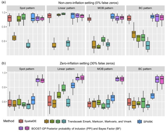
Simulation study: The boxplots of AUCs achieved by BOOST-GP, SPARK, SpatialDE and Trendsceek under different scenarios in terms of spatial pattern and count generating process

Regarding the efficiency, the average execution time per gene was 0.171, 0.003 and 4.413 s for SPARK, SpatialDE and Trendsceek. Note that Trendsceek conducted four tests (i.e. Emark, Markcorr, Markvario and Vmark) together, so it took longer. BOOST-GP spent 10.320 s per gene on average due to the computationally intensive MCMC algorithms, even though it was written by Rcpp to accelerate computation. All experiments were implemented on a high performance computing server with two Intel Xeon CPUs (45 MB cache and 2.10 GHz) and 250 GB memory.

5 Real data analysis

We applied BOOST-GP to analyze two published SMP datasets generated by STS, the MOB and human BC, accessible on Spatial Research Lab (https://www.spatialresearch.org/). These data consist of gene-expression measurements in the form of read counts collected on a number of spatial locations known as spots. There are 12 replicates and 4 layers available for MOB and BC cohorts, respectively. Following the previous studies (Sun et al., 2020; Svensson et al., 2018), we used the MOB replicate 11, which contains 16 218 genes measured on 262 spots, and the BC layer 2, which contains 14 789 genes measured on 251 spots. We applied the same quality control steps suggested by Sun et al. (2020) to remove outlier genes and spots. After filtering out those spots with fewer than 10 total counts across all genes and those genes with more than 90% zero read counts across all spots, the MOB data had p = 11 274 genes and n = 260 spots, while the BC data had p = 5262 genes and n = 250 spots. We applied the same prior specification, algorithm setting and significance criteria that we used in the simulation. Because of the poor performance of Trendsceek in simulation studies, we did not include it in real data analysis.

We checked the MCMC algorithm convergence based on the PPI vector of $\mathit{\gamma }$. We calculated the PPIs for all the four chains and found their pairwise Pearson correlation coefficients ranged from 0.934 to 0.988, suggesting good MCMC convergence. We then aggregated the outputs of all chains. Figure 4 shows the overlap of identified SV genes by SpatialDE, SPARK and BOOST-GP methods in MOB and BC datasets. SPARK was shown to be the most aggressive method that reported the most SV genes, while SpatialDE was the most conservative one and reported the fewest SV genes. BOOST-GP lay in between SpatialDE and SPARK, with a lot in common with them, but also uniquely identified genes. Because SpatialDE was almost always a subset of SPARK, we focused on the comparison between BOOST-GP and SPARK in the following analysis. We then did hierarchical clustering on the SV genes identified by BOOST-GP and SPARK, and plotted the averaged normalized expression levels within each cluster to represent each pattern.

Fig. 4.

Real data analysis: the Venn diagram of SV genes identified by BOOST-GP, SPARK, and SpatialDE in (a) MOB and (b) human BC data

In order to have a more detailed comparison and not overshadow any subtle patterns, we clustered those SV genes of MOB, as shown in Figure 5a and b, into six and four groups. We could see that in MOB data, the patterns detected by BOOST-GP and SPARK resemble each other well. More specifically, the first to sixth patterns can be further merged, leading to three major patterns, which was consistent with what was reported by Sun et al. (2020). This suggested that although BOOST-GP detected fewer SV genes than SPARK, it did not miss any major patterns. In BC data, the patterns summarized by the two methods showed more distinctiveness, especially the first pattern. The remaining three patterns could still largely overlap each other, though not perfectly. This agreed with the Venn diagram that more discrepancy was found between BOOST-GP and SPARK in BC data compared to the MOB data.

Fig. 5.

Real data analysis: (a) and (b) the averaged normalized gene-expression levels of SV genes identified by BOOST-GP and SPARK in (a) MOB and (b) human BC data, respectively. (c) and (d) The associated hematoxylin and eosin-stained tissue slides of MOB and BC data, respectively

To have an additional diagnosis of the spatial signals of the detected SV genes, we employed Moran’s I spatial autocorrelation test (Li et al., 2007; Moran, 1950) (detailed in the Supplementary Material). Its values range from –1 to 1. The larger the Moran’s I, the stronger the spatial correlation, which means clustering spots with similar normalized expression levels. Supplementary Figure S2 displays three binary spatial pattern examples with different values of Moran’s I. Figure 6a summarized the Moran’s I’s of the common SV genes found by both methods and SV genes found by individual method alone. Spatial autocorrelation was shown to be the strongest in the common SV gene set, followed by the BOOST-GP only set and then the SPARK only set. The result implies: (i) SV genes identified by both methods are more likely to be true SV genes and (ii) SPARK were in general more aggressive to report more candidates but also with lower average signals. This might be because SPARK considered two types of kernels (SE and periodic) and used five characteristic length-scales for each kernel (i.e. 10 kernels in total), which caused more versatility. Moreover, SPARK did not take zero-inflation into account, which tended to report more FP discoveries.

Fig. 6.

Real data analysis: (a) the boxplots of Moran’s I’s of SV genes identified by both BOOST-GP and SPARK, BOOST-GP only and SPARK only. (b) and (c) The averaged normalized gene-expression levels of SV genes identified by BOOST-GP only and SPARK only in MOB and human BC data, respectively

In parallel, we also performed hierarchical clustering on these three sets of genes. In MOB data, 680 genes identified by SPARK only could be clustered into four groups, as shown in Figure 6b, same as the ones previously described in Figure 5a, while the 45 genes identified by BOOST-GP only mainly belonged to two patterns, as shown in Figure 6b. This result suggested SPARK might be more sensitive in MOB data, as it is able to find some weak signal genes, but in the meantime, according to Figure 6a, some of those could potentially be FPs that lead to the dilution of Moran’s I’s. In BC data, 372 genes identified by SPARK only showed both much weaker spatial signals and less spatial patterns compared to 108 genes identified by BOOST-GP only, as shown in Figure 6c, suggesting the SPARK method potentially scarified specificity while it did not capture TPs as well.

Last, we conducted gene ontology (GO) enrichment analysis using a Python wrapper GSEAPY (Kuleshov et al., 2016; Subramanian et al., 2007) to see whether those detected SV genes by BOOST-GP were related to certain biological functions. GSEAPY can be accessible on https://gseapy.readthedocs.io/en/latest/. We performed this on 2941 mouse and 2338 human GO terms of biological processes, which had at least one gene overlap with detected SV gene pools. Using the adjusted P-value smaller than 0.05 as the threshold, we found 148 and 197 enriched biological process GO terms in MOB and BC datasets. We took a closer look at those terms that were associated with the synaptic and nervous system for MOB data, as they play important roles in synaptic organization and nerve development, which is expected to be involved in olfactory functioning. As showed in Figure 7, many of those synaptic- and nervous-related GO terms were significantly enriched, suggesting the functions of those detected SV genes were aligned with the underlying mechanism that drove the spatially differentiated expression pattern. This was consistent with what was reported in Sun et al. (2020). For BC data, the terms related to extracellular matrix and immune response, as expected, were found to be significantly enriched in the identified SV genes, as they are over-activated in BC. Furthermore, five ERBB-related pathways were found to be significant in our analysis. ERBB family genes, especially ERBB2, are well-known oncogenes in BC that have a close relationship with altered signaling pathways and tumorigenesis and development (Stern, 2000). Three of them were displayed in Figure 7. However, none of them were found significant in the SPARK analysis result [e.g. the adjusted P-value for ERBB2 signaling pathway (GO: 0038128) was 0.239]. We went back and had a deeper check. We found the reason was some genes involved in ERBB pathway were significant in BOOST-GP result but only marginally significant in SPARK (e.g. the adjusted P-value and PPI of gene UBB were $9.22\times {10}^{16}$ and 0.650 reported by BOOST-GP, the corresponding adjusted P-value for SPARK and SpatialDE were 0.053 and 0.857). It echoed with the previous clustering and autocorrelation analysis, where BOOST-GP had more reliable results in BC data than SPARK.

Fig. 7.

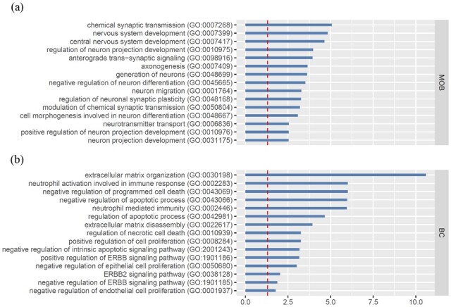
Real data analysis: GO enrichment analysis of SV genes identified by BOOST-GP in (a) MOB and (b) human BC data. The red dashed line indicates a significant level of 0.05

6 Conclusion

Recently, the emerging SMP technologies demonstrated great potential in revealing tissue spatial organization and heterogeneity. In this study, we developed a novel Bayesian hierarchical model that incorporates a GP model to identify SV genes. It can also characterize the embedded temporal or spatial patterns in high-resolution time-series RNA-Seq data (e.g. Owens et al., 2016) or three-dimensional SMP data (e.g. Shah et al., 2016). Compared to other existing methods, it has several advantages. First, it directly models count data with an NB distribution that could accommodate the over-dispersion compared to the Poisson distribution. Second and most importantly, it properly addresses the excess of zero count problem, which is typically observed in the SMP data, using a zero-inflation model. Third, it improves the estimation of the kernel length-scale parameter using a Bayesian approach, leading to more stable and accurate results. In simulation studies, BOOST-GP had similar power in identifying SV genes compared with SpatialDE and SPARK, and much better than Trendsceek in general spatial settings. It greatly outperformed all other methods when false zeros were present in the data. In real data, BOOST-GP and SPARK both had reasonable performance and had a lot in common, while SpatialDE was a bit conservative. The performance of different methods may vary in different datasets with different inherent spatial patterns and data structures. SPARK seemed to be more sensitive in MOB data with some sacrifice in precision. BOOST-GP performed better in human BC data, identifying undiscovered spatial patterns and meaningful enriched pathways. In general, SPARK was a more aggressive method under the selected significance cutoff, but at the same time bearing a higher risk of discovering more FPs. Because BOOST-GP reports both marginal PPI and BFs (which could be converted to P-values under some assumption) as measures of significance, users have more freedom to balance the sensitivity and specificity on their own considerations depending on the study needs.

Several extensions of our model are worth investigating. Firstly, with a Bayesian framework, BOOST-GP can be further extended to incorporate pathway information as prior knowledge to take into account the regulatory relationships between genes to perform a joint estimation. Secondly, the choice of an appropriate kernel function is of critical importance in spatial modeling (Rasmussen, 2003). We used only the SE kernel in BOOST-GP. However, the related covariance function is infinitely differentiable, making a spatial pattern too smooth to be realistic. In the future, we would consider the Matérn and rational quadratic kernels suggested by Stein (2012), which are suitable for both weak and strong smoothness assumptions.

References

- Airoldi E.M., Bischof J.M. (2016) Improving and evaluating topic models and other models of text. J. Am. Stat. Assoc., 111, 1381–1403. [Google Scholar]
- Banerjee S. et al. (2014) Hierarchical Modeling and Analysis for Spatial Data. CRC Press, Boca Raton, USA. [Google Scholar]
- Benjamini Y., Hochberg Y. (1995) Controlling the false discovery rate: a practical and powerful approach to multiple testing. J. R. Stat. Soc. Series B Stat. Methodol., 57, 289–300. [Google Scholar]
- Cameron A.C., Trivedi P.K. (2013) Regression Analysis of Count Data. Vol. 53. Cambridge University Press, Cambridge, UK. [Google Scholar]
- Chen K.H. et al. (2015) Spatially resolved, highly multiplexed RNA profiling in single cells. Science, 348, aaa6090. [DOI] [PMC free article] [PubMed] [Google Scholar]
- Diggle P.J. et al. (1998) Model-based geostatistics. J. R. Stat. Soc. Series C Appl. Stat., 47, 299–350. [Google Scholar]
- Edsgärd D. et al. (2018) Identification of spatial expression trends in single-cell gene expression data. Nat. Methods, 15, 339–342. [DOI] [PMC free article] [PubMed] [Google Scholar]
- Eng C.-H.L. et al. (2019) Transcriptome-scale super-resolved imaging in tissues by RNA seqFISH+. Nature, 568, 235–239. [DOI] [PMC free article] [PubMed] [Google Scholar]
- Finak G. et al. (2015) MAST: a flexible statistical framework for assessing transcriptional changes and characterizing heterogeneity in single-cell RNA sequencing data. Genome Biol., 16, 278. [DOI] [PMC free article] [PubMed] [Google Scholar]
- Gelfand A.E., Schliep E.M. (2016) Spatial statistics and Gaussian processes: a beautiful marriage. Spat. Stat., 18, 86–104. [Google Scholar]
- Kass R.E., Raftery A.E. (1995) Bayes factors. J. Am. Stat. Assoc., 90, 773–795. [Google Scholar]
- Kharchenko P.V. et al. (2014) Bayesian approach to single-cell differential expression analysis. Nat. Methods, 11, 740–742. [DOI] [PMC free article] [PubMed] [Google Scholar]
- Kuleshov M.V. et al. (2016) Enrichr: a comprehensive gene set enrichment analysis web server 2016 update. Nucleic Acids Res., 44, W90–W97. [DOI] [PMC free article] [PubMed] [Google Scholar]
- Li H. et al. (2007) Beyond Moran’s I: testing for spatial dependence based on the spatial autoregressive model. Geogr. Anal., 39, 357–375. [Google Scholar]
- Li J. et al. (2012) Normalization, testing, and false discovery rate estimation for RNA-sequencing data. Biostatistics, 13, 523–538. [DOI] [PMC free article] [PubMed] [Google Scholar]
- Li Q. et al. (2017) A Bayesian mixture model for clustering and selection of feature occurrence rates under mean constraints. Stat. Anal. Data Min., 10, 393–409. [Google Scholar]
- Li Q. et al. (2019) Bayesian negative binomial mixture regression models for the analysis of sequence count and methylation data. Biometrics, 75, 183–192. [DOI] [PubMed] [Google Scholar]
- Love M.I. et al. (2014) Moderated estimation of fold change and dispersion for RNA-seq data with DESeq2. Genome Biol., 15, 550. [DOI] [PMC free article] [PubMed] [Google Scholar]
- Lubeck E. et al. (2014) Single-cell in situ RNA profiling by sequential hybridization. Nat. Methods, 11, 360–361. [DOI] [PMC free article] [PubMed] [Google Scholar]
- Lun A.T. et al. (2016) Pooling across cells to normalize single-cell RNA sequencing data with many zero counts. Genome Biol., 17, 75. [DOI] [PMC free article] [PubMed] [Google Scholar]
- Marioni J.C. et al. (2008) RNA-seq: an assessment of technical reproducibility and comparison with gene expression arrays. Genome Res., 18, 1509–1517. [DOI] [PMC free article] [PubMed] [Google Scholar]
- Matthews B.W. (1975) Comparison of the predicted and observed secondary structure of T4 phage lysozyme. Biochim. Biophys. Acta, 405, 442–451. [DOI] [PubMed] [Google Scholar]
- Moffitt J.R. et al. (2018) Molecular, spatial, and functional single-cell profiling of the hypothalamic preoptic region. Science, 362, eaau5324. [DOI] [PMC free article] [PubMed] [Google Scholar]
- Moran P.A. (1950) Notes on continuous stochastic phenomena. Biometrika, 37, 17–23. [PubMed] [Google Scholar]
- Newton M.A. et al. (2004) Detecting differential gene expression with a semiparametric hierarchical mixture method. Biostatistics, 5, 155–176. [DOI] [PubMed] [Google Scholar]
- Owens N.D. et al. (2016) Measuring absolute RNA copy numbers at high temporal resolution reveals transcriptome kinetics in development. Cell Rep., 14, 632–647. [DOI] [PMC free article] [PubMed] [Google Scholar]
- Rasmussen C.E. (2003) Gaussian processes in machine learning. In: Summer School on Machine Learning. Springer, Berlin, Germany, pp. 63–71. [Google Scholar]
- Roberts S. et al. (2013) Gaussian processes for time-series modelling. Philos. Trans. R. Soc. A, 371, 20110550. [DOI] [PubMed] [Google Scholar]
- Robinson M.D. et al. (2010) edgeR: a Bioconductor package for differential expression analysis of digital gene expression data. Bioinformatics, 26, 139–140. [DOI] [PMC free article] [PubMed] [Google Scholar]
- Rodriques S.G. et al. (2019) Slide-seq: a scalable technology for measuring genome-wide expression at high spatial resolution. Science, 363, 1463–1467. [DOI] [PMC free article] [PubMed] [Google Scholar]
- Shah S. et al. (2016) In situ transcription profiling of single cells reveals spatial organization of cells in the mouse hippocampus. Neuron, 92, 342–357. [DOI] [PMC free article] [PubMed] [Google Scholar]
- Ståhl P.L. et al. (2016) Visualization and analysis of gene expression in tissue sections by spatial transcriptomics. Science, 353, 78–82. [DOI] [PubMed] [Google Scholar]
- Stein M.L. (2012) Interpolation of Spatial Data: Some Theory for Kriging. Springer Science & Business Media, Berlin, Germany. [Google Scholar]
- Stern D.F. (2000) Tyrosine kinase signalling in breast cancer: ErbB family receptor tyrosine kinases. Breast Cancer Res., 2, 1–8. [DOI] [PMC free article] [PubMed] [Google Scholar]
- Subramanian A. et al. (2007) GSEA-P: a desktop application for gene set enrichment analysis. Bioinformatics, 23, 3251–3253. [DOI] [PubMed] [Google Scholar]
- Sun S. et al. (2020) Statistical analysis of spatial expression patterns for spatially resolved transcriptomic studies. Nat. Methods, 17, 193–200. [DOI] [PMC free article] [PubMed] [Google Scholar]
- Svensson V. et al. (2018) SpatialDE: identification of spatially variable genes. Nat. Methods, 15, 343–346. [DOI] [PMC free article] [PubMed] [Google Scholar]
- Tadesse M.G. et al. (2005) Bayesian variable selection in clustering high-dimensional data. J. Am. Stat. Assoc., 100, 602–617. [Google Scholar]
- Williams C.K., Rasmussen C.E. (2006) Gaussian Processes for Machine Learning. Vol. 2. MIT Press, Cambridge, MA. [Google Scholar]
- Witten D. et al. (2010) Ultra-high throughput sequencing-based small RNA discovery and discrete statistical biomarker analysis in a collection of cervical tumours and matched controls. BMC Biol., 8, 58. [DOI] [PMC free article] [PubMed] [Google Scholar]
- Witten D.M. (2011) Classification and clustering of sequencing data using a Poisson model. Ann. Appl. Stat., 5, 2493–2518. [Google Scholar]
- Zhang M. et al. (2021) Spatial molecular profiling: platforms, applications and analysis tools. Brief. Bioinform., 22, bbaa145. [DOI] [PMC free article] [PubMed] [Google Scholar]
Associated Data
This section collects any data citations, data availability statements, or supplementary materials included in this article.