Osteoporosis diagnosis in knee X-rays by transfer learning based on convolution neural network

Abstract

Osteoporosis degrades the quality of bones and is the primary cause of fractures in the elderly and women after menopause. The high diagnostic and treatment costs urge the researchers to find a cost-effective diagnostic system to diagnose osteoporosis in the early stages. X-ray imaging is the cheapest and most common imaging technique to detect bone pathologies butmanual interpretation of x-rays for osteoporosis is difficult and extraction of required features and selection of high-performance classifiers is a very challenging task. Deep learning systems have gained the popularity in image analysis field over the last few decades. This paper proposes a convolution neural network (CNN) based approach to detect osteoporosis from x-rays. In our study, we have used the transfer learning of deep learning-based CNNs namely AlexNet, VggNet-16, ResNet, and VggNet −19 to classify the x-ray images of knee joints into normal, osteopenia, and osteoporosis disease groups. The main objectives of the current study are: (i) to present a dataset of 381 knee x-rays medically validated by the T-scores obtained from the Quantitative Ultrasound System, and (ii) to propose a deep learning approach using transfer learning to classify different stages of the disease. The performance of these classifiers is compared and the best accuracy of 91.1% is achieved by pretrained Alexnet architecture on the presented dataset with an error rate of 0.09 and validation loss of 0.54 as compared to the accuracy of 79%, an error rate of 0.21, and validation loss of 0.544 when pretrained network was not used.. The results of the study suggest that a deep learning system with transfer learning can help clinicians to detect osteoporosis in its early stages hence reducing the risk of fractures.

Introduction

X-ray imaging is the most common imaging technique amongst the medical community to find bone pathologies. X-rays are the oldest and most common techniques to take images of almost all bones of the body like wrist, knee, elbow, shoulder, knee, pelvis, spine, etc. X-ray imaging helps in fracture diagnosis, dislocation of joints, bone injury, abnormal bone growth, infection, and even arthritis. Bone fractures are usually accidental but they can be pathological also. That is due to the weakening of bones caused by osteoporosis, cancer, or osteogenesis. Osteoporosis is the leading bone pathology causing millions of fractures worldwide [29] and women are more affected [30]. Osteoporosis is related to age as bones become weak with the advancing age but sometimes osteoporosis prevails at younger ages also [9]. Osteoporosis is also termed as the silent disease because its symptoms are not visible in the early stages and they get prevalent when osteoporosis has reached the very advanced stage where bones are susceptible to fractures with just a little fall. The fracture fixation and other treatment costs of osteoporosis take a huge amount of budget from the economies [4, 46]. So, to reduce the treatment cost it needs to be diagnosed in the early stages.

Medically osteoporosis is diagnosed with Dual Energy X-ray Absorptiometry Technique (DXA) [13]. which determines the bone mineral density (BMD) in terms of the T-score and Z-score values approved by WHO for different stages of osteoporosis [65]. But it suffers from some limitations which include areal measurements with the technique being costly and less available. Other imaging modalities that are used for osteoporosis detection are the Quantitative Ultrasound System (QUS) [19, 21], Computed Tomography (CT) [6, 28], Magnetic Resonance Imaging (MRI) [7, 18]. MRI is a 3 T improved bone microarchitecture imaging technology but is very costly and has lower spatial resolution [7, 18], CT is 3D geometric imaging with volumetric measurements but has a high dose of radiation and doesn’t qualify for the WHO’s definition of osteoporosis detection [6, 28]. QUS is simple, non-invasive, portable, cost-effective, and uses sound waves for studying bones but it is site-specific and has an absence of strong empirical evidence [19, 21]. Considering these limitations, a cost-effective, readily available, and accurate detection system is required. This led the researchers to take advantage of recent advancements in the field of imaging technology to analyze medical images with computer algorithms to form computer-aided diagnostic systems (CAD).

In recent years, among the CAD systems for medical image analysis, deep learning-based convolutional neural network (CNN) techniques have gained popularity [38, 66] due to their state-of-the-art results in detecting many diseases from images like brain tumor detection [41], breast cancer detection [8], pneumonia detection [47], cancer detection [48, 49], human activity recognition [2], multiple sclerosis [3] etc. CNNs like AlexNet, ResNet-50, VGG-16, VGG-19, and GoogleNet [23, 33, 51, 56] have shown state-of-the-art results in the classification of medical images. The main challenge in using CNN classifiers is that they need a huge amount of labeled data for training but in the medical field availability of a big-size dataset is very difficult. To address this issue researchers have come up with the idea of transfer learning [60]. In transfer learning, a CNN trained on a huge dataset is retrained with a smaller dataset of a new problem, and CNN uses the knowledge gained from a huge dataset to easily learn the features of the new small dataset and thus effectively helps in classifying the images.

Many CAD systems are proposed for osteoporosis diagnosis including deep learning at various bone sites like hip, spine, hand, and tooth but not much work has been done to detect knee osteoporosis [62, 63]. The knee is the most stressed joint, bearing the weight of the body and responsible for mobility. With the increase in the aged population, the incidence of osteoporotic fractures around the knee increases with women at more risk of tibial and fibular fractures [10]. It is estimated that around half of the knee fractures occur in patients which are older than 50 yrs. of age and in the elderly patients who sustain femoral fractures, with less function and low quality of life, a high 1-year mortality rate of 22% is noted [53]. An early detection system is needed to detect the prevalence of osteoporosis in the knee bone to prevent fractures and reduce treatment costs [1, 44, 61].

In this paper, we have used the power of CNN architectures and the cost-effectiveness of X-ray imaging to find the early detection system for knee osteoporosis. Our model uses the prominent CNNs namely AlexNet, VggNet-16, ResNet, and VggNet-19 for classifying the knee X-ray Images.

The main contributions of our study are summarised below:

• A labelled dataset of knee X-rays classified as normal, osteopenic, and osteoporotic according to the T-score measured by the QUS system is presented.

• Four prominent CNN networks (AlexNet, VggNet-16, ResNet, and VggNet −19) are considered for experimentation using the PyTorch library known as Fastai [23].

• The transfer learning is applied in all CNN networks and results are compared to find the most appropriate network to be used in clinical practices for osteoporosis detection.

• To the best of our knowledge, this is the first study to detect osteoporosis in knee bone with the labeled dataset having all three classes of osteoporosis i.e.; normal, osteopenia, and osteoporosis.

The rest of the paper is organized as related work is discussed in Section 2. In Section 3, we have discussed the dataset used in the study with the different methods used to study the dataset. Section 4 presents the experimentation and results and Section 5 discusses and compares the results with existent works of literature. Finally, Section 6 concludes the paper and shows the limitations of the study and future directions.

Related work

Machine learning approaches especially deep convolution neural networks have shown state-of-the-art results in disease detection [15]. Many researchers have successfully used machine learning approaches to build the osteoporosis diagnosis system from different types of images [63]. In this section, we have discussed the latest works done in the field of osteoporosis diagnosis using deep convolution neural networks.

Computed radiography images were utilized in [22] in 2016 to detect osteoporosis from phalanges with DCNN. They used three-fold cross-validation for evaluation and achieved a good diagnosis ratio.

Naoufami et al. [59] in their work proposed DCNN to detect osteoporotic vertebral fractures (VF). Computed tomographic images of vertebrae were used to extract logical features and then the performance of the system was compared with the practicing radiologists and comparable results were achieved. Derkatch et al. [12] used DCNN to detect vertebral fractures from DXA images with good accuracy. CT scans of vertebrae were utilized by Krishnaraj et al. [32] to identify osteoporotic and non-osteoporotic subjects. They used U-net CNN for the segmentation of CT images and achieved good accuracy. Vertebral CT scans were also utilized by Fang et al. [16] for osteoporosis detection. They used DenseNet-121 CNN classifier to classify normal and osteoporotic vertebrae. DCNN was also employed by Zhang et al. to detect osteoporosis and osteopenia in lumbar spine radiographs they included that dataset containing the images of only women aged ≥50 [71]. Lee et al. [36] extracted the spine x-rays features with the help of CNN architectures and passed them to the machine learning classifiers for classification. They achieved the maximum classification accuracy of 71% with VGG for feature extraction and random forest for classification. Yasaka et al. [68] used the CNN architecture to predict the BMD of lumbar vertebrae from computed tomography images of the abdomen. They found a good correlation between the predicted BMD from CNN and the DXA BMD. Computed tomography scans of the spine were studied by Sollmann et al. [52] and assessed the volumetric bone mineral density with CNN. They compared the results with the volumetric bone mineral density obtained from routine CT and found that CNN gives high diagnostic accuracy.

Dental Panoramic Radiographs (DPRs) were utilized by Lee et al. [35] to diagnose osteoporosis from the tooth with the help of a convolution neural network. The results of oral and maxillofacial radiologists were surpassed by this DCNN. DPRs were also used by [37] for osteoporosis detection. They used VGG-16 CNN classifier and employed transfer learning in VGG-16 to improve the classification performance of the CNN classifier. AlexNet CNN was used by Yu et al. [70] to detect osteoporosis from dental Panoramic radiographs. They classified the DPRs in osteoporotic and non-osteoporotic with good accuracy but doesn’t include the osteopenia class exclusively. DPRs were also studied by Sukegawa et al. [54] with the help of CNNs to detect osteoporosis on and found the good performance. They also added the clinical covariates which further improved the classification performance.

The magnetic resonance images of the proximal femur were studied by Deniz et al. [11] for osteoporosis detection. They used DCNN to segment the proximal femur for measuring the quality of bone and assessment of fracture.

Two CNN models namely MS-Net (Mark- Segmentation- Network) and BCC-Net (Bone- Conditions -Classification Network) were proposed by Tang et al. [57] for ROI selection and for bone type determination on basis of extracted features from ROI respectively in osteoporosis diagnosis and achieved 76.65% accuracy.

Liu et al. [40] diagnosed osteoporosis from x-ray images of the pelvis. They calculated the energy function from the softmax of the proposed U-net model that uses the deep features of the medullary joint from X-rays to detect osteoporosis. This study poorly diagnoses the images of the bone mass reduction group and osteoporosis group. Yamamoto et al. [67] detected osteoporosis from hip radiographs using CNN. They combined the clinical covariates with images and found that it improved the performance and the best performance was achieved by EfficeientNet CNN.

The AlexNet Classifier was used by Tecle et al. for diagnoses of osteoporosis [58]. They used the X-ray images of the hand and classified the osteoporotic and non-osteoporotic images from the segmented second metacarpal region.

He et al. [24] analysed the knee X-rays and proposed to use two radiographic parameters namely cortical bone thickness and distal femoral cortex for bone quality assessment. These parameters were found to have a significant correlation with BMD and T-score.

From the above-related works of literature, we could find that knee osteoporosis is an under-studied field as compared to other sites like vertebrae and teeth. Detecting osteoporosis from the knee can protect vital organs like kidney, pancreas, etc. from getting exposed to harmful radiation while getting the images for analysis. X-rays are also the cheapest form of medical images available and can help build a cost-effective system. we have used the knee x-ray images which are classified as normal, osteopenic, and osteoporotic on basis of T-score values obtained from the QUS system to train the CNN networks. The transfer learning helps the CNN to perform well even when trained on a small dataset.

Materials and methods

Dataset

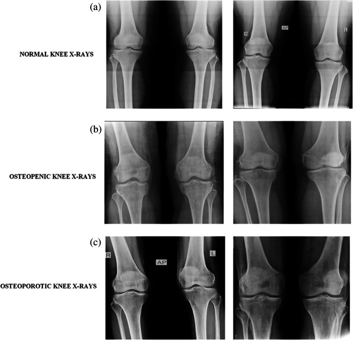
The knee x-ray images were collected from the BMD camp organized by the Unani and Panchkarma Hospital, Srinagar, J&K, India, and its sister branches from 21 to 12-2019 to 31-12-2019 in central Kashmir, north Kashmir, and south Kashmir. The camp was organized in the hospital premises and was open to participants from all age groups, genders, and different regions of Kashmir, India. The dataset consists of both x-ray images as well as osteoporosisrelated clinical factors for each participant. Each patient first went through a personal interview wherein he was informed about the procedure of the QUS BMD test and various clinical factors like age, gender, height, previous history of fracture or any other pathology, lifestyle habits, medications, etc. were documented. Written consent from each participant was taken for using their data without their personal details like name, and address in the research study. Then the BMD was measured just below the knee with the peripheral bone assessment QUS system known as the Sunlight Omnisense 7000S with simulation software from Pegasus Prestige (Osteomed, DMS, France). The QUS system was chosen as it is radiation-free, multisite, easy to use, affordable, accurate, portable, and fits the osteoporosis diagnosis criteria of WHO [17]. The report generated with this QUS system contains the Z-score value, T-score value, diagnosis i.e.; normal, osteopenia or osteoporosis, and area of assessment for measuring the BMD. After the BMD measurement, the knee x-rays in anteroposterior view (AP) were taken from the participants who gave consent to undergo an x-ray. Among the total of 932 participants who went through the BMD test, only 240 gave consent to undergo the x-ray scanning. The x-rays obtained were then kept under the different classes of BMD level on basis of the T-score values recommended by WHO obtained from the QUS system. The BMD tests of the participants confirmed that among the 240 participants, ones with normal BMD were 37 with 18 males and 19 females; 154 were osteopenic with 59 males and 95 females; 49 were osteoporotic with 31 males and 18 females. The dataset is available at [43]. The demographic information of the 240 participants is given in Table 1 with sample knee x-rays from normal, osteopenic, and osteoporotic classes shown in Fig. 1 [64].

Table 1.

Demographic information like lifestyle factors, clinical factors, and no. of samples in QUS classified Classes for the dataset. BMI: body mass index

Variables		Values
Males		108
Females		132
		Males	Females
Normal subjects		18	19
Osteopenic subjects		59	95
Osteoporotic subjects		31	18
Age group (years)
1st group	<18	1	0
2nd group	18–30	5	12
3rd group	31–45	18	39
4th group	46–60	42	72
5th group	61–75	40	9
6th group	>75	2	0
Mean age		51
Standard Deviation of age		13
Mean height (m)		2
Standard deviation of height		0.096
Mean weight (kg)		69.1
Standard deviation of weight		9.6
BMI mean		28
BMI standard deviation		4
Obesity		Normal weight	Overweight	Obese
		58	112	67
No smokers			41
No of postmenopausal women			83
History of Fracture			61
Family history of osteoporosis			66
Diabetic Participants			12
Thyroidic Participants			34

Fig. 1.

Sample images from the database from top to bottom (a) normal X-ray, (b) Osteopenia X-ray, (c) Osteoporosis X-ray

In the x-rays collected from the camp, some X-rays had scans of both the knees so, the left and right knee x-rays were separated and then the dimensions of all the x-rays were kept the same, and finally, we have 381 knee x-rays. The region of interest containing the knee joint and some area from the top and bottom limb was extracted from each x-ray to be used for further processing. In this study, we have used only the x-ray images from the database to make the vision-based classification system from CNNs. The image dataset was further split into training and validation sets. The CNNs AlexNet, Resnet-50, VggNet-16, and VggNet-19 are trained with the training set and the accuracy of the classifier is then validated with the validation sets.

Proposed methodology

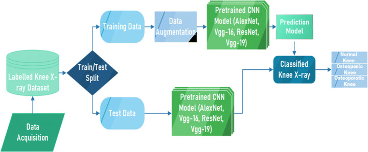
Figure 2 shows the block diagram of proposed model for detection of osteoporosis from knee x-rays. Firstly, the knee X-rays were collected as mentioned in Section 3.1 to form an image dataset which is then split into training data (used to train CNN classifier) and test data (used to test the trained classifier). The training data is augmented to increase the number of images in the training set as CNN works better with more data. Then the imageset is passed on to CNN model for training the CNN. Then finally the prediction ratio of train and test data is analysed and performance of classifier to classify images into normal, osteopenia, and osteoporostic images is evaluated.

Fig. 2.

Block Diagram of Proposed Methodology

CNN architectures

CNN is the variant of deep neural networks whose intermediate levels are based on the principle of convolution. The convolution is the mathematical function in which one function is modified with another function to get a new function with some modified features. CNNs are used for the processing of images in which the image is convolved with a filter of less length * width to reduce the size of the images but maintain the basic information contained in the image. CNN as compared to other deep learning architectures have received more interest from researchers because they can utilize both the configural and the spatial information of the 2D as well as 3D images [34]. The source of power in CNN is that it can learn the image data directly from the image without any extra methods required for feature extraction as in other machine learning methods [27] or object segmentation [55]. Many CNNs have been developed to solve various types of problems and they vary with each other in one or the other aspect but the basic components are the same. The CNNs consist of three types of layers viz.; convolutional layer, pooling layer, and fully connected layer. The convolutional layer is responsible for learning the feature representations of the input images by using the set of filters. The pooling layer helps in reducing the computations and parameters with the downsampling of the representations to achieve the shift-invariance. It is usually placed in between the two convolutional layers. There could be any number of convolutional and pooling layers in the network. By stacking them properly we can extract the feature maps containing the higher-level representations. One or more fully connected (FC) layers are present at the end of the stacked convolutional and pooling layers and before the output layer, to perform the task of reasoning.

In our study, we have employed the popular pretrained CNN architectures namely AlexNet, ResNet-18, VggNet-16, and VggNet-19.

AlexNet

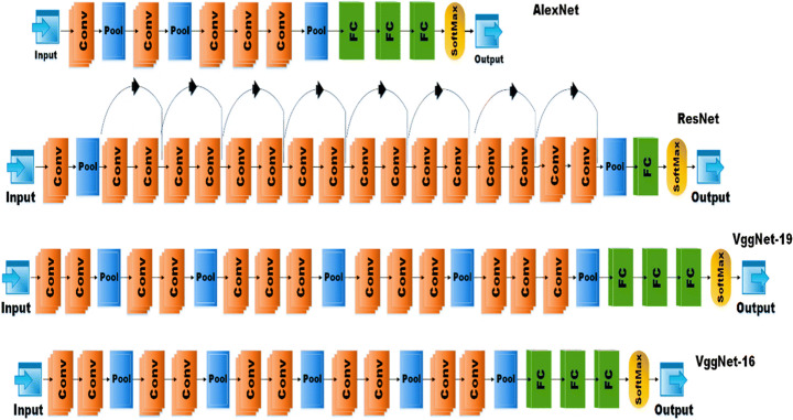
AlexNet proposed by Krizhevsky et al. is known for its breakthrough in machine learning for achieving high accuracy in the classification of 1.2 million HR (high resolution) images at ImageNet LSVRC-2010 contest in 1000 different classes with a 15.3% of top error rate. It outperformed the previous state-of-the-art architectures. The network consists of 5 convolutional neural networks followed by max-pooling layers and then three fully connected layers with a 1000-way softmax classifier at the end. The basic architecture of AlexNet from [33] is shown in Fig. 3. AlextNet has been used in many applications to classify different types of images. In disease detection from medical images, AlexNet has shown efficient results and outperformed the expertise of medical experts in many applications like brain tumor detection from brain MRI [42], skin lesion detection [25], COVID -19 [50], etc. AlexNet was chosen for this comparison as its training speed is 5 times faster than other DL architectures, it works with any GPU with no extra hardware requirement, and uses a RELU activation function that can converge the stochastic gradient descent with good acceleration [25].

Fig. 3.

Basic Network architecture of AlexNet, ResNet-18, VggNet-19, and VggNet-16.Fastai

ResNet-18

ResNet CNN architecture, proposed by He et al. [23] won the ILSVC challenge of 2015 bringing the error rate as low as 3.6%. It was an extremely deep network with 152 layers. ResNets are built on multiple stocks of residual blocks. Residual blocks help to feed the activation of one layer to the layer deeper in the network by using skip connections. This helps the system train faster. ResNet has many variants like ResNet-18, ResNet-34, ResNet-50, ResNet-101, ResNet-152 as per the number of layers in the network. In our study, we have used the ResNet −18 architecture as our dataset is not so large. The network architecture for ResNet −18 is given in Fig. 3. In medical image classification ResNet has shown very promising results in detecting brain pathology [39], Thyroid Ultrasound images [20], breast cancer detection [69], etc.

VggNet

VggNet CNN architecture, proposed by Simonyan et al. [51] of the Visual Geometry Group of Oxford University and was the first runner-up in the ILSVR challenge of 2014. The main aspect of VggNet is its cascading network architecture. it uses small 3✕3 convolution filters and a pooling layer after 2 or 3 convolutional layers. The network has two variants on basis of the number of convolution, pooling, and fully connected layers i.e. 16 or 19 known as VggNet-16 and VggNet-19 models respectively. The general architecture of VggNets is given in Fig. 2. In medical diagnosis, VggNet has shown the state of the art results in detecting many diseases from medical images like diabetic retinopathy [31], Alzheimer’s disease detection [14], malaria disease detection [45], etc.

The model architecture layers and basic features of AlexNet, VggNet-16, ResNet, and VggNet-19 are given in Table 2.

Table 2.

The table depicts the number of convolution, pooling layers, FC layers, and basic features of AlexNet, VggNet-16, ResNet-18, and VggNet-19 architectures

Model	Year	No. of Covoluti on Layers	No. of Pooling Layers	Fully Connect ed Layers	Main Features
AlexNet	2012	5	3	3	▪ First CNN architecture to win ImageNet challenge with top-5 error rate of 15.3%.
					▪ Used ReLU as activation function instead of tanh or sigmoid.
					▪ AlexNet has 60 million parameters.
					▪ It had used the Stochastic Gradient descent as the learning algorithm.
VggNet-16	2014	13	5	3	▪ The model achieved 92.7% top-5 test accuracy in ImageNet challenge.
					▪ The model replaces the the large sized kernals used in AlexNet with 3✕3 sized multiple kernals enabling better learning.
					▪ Main con of this network is that it is slow to train.
					▪ And network architecture weights are quite large.
ResNet	2015	17 with 8 residual units	2	1	▪ Main building blocks are residual blocks that increase the performance of the network.
					▪ The identity connection helps the network to handle vanishing gradient problem.
					▪ The batch normalisation used by network mitigates the problem of covariant shift.
					▪ ResNet 18 has residual blocks of two layers deep.
VggNet-19	2014	16	5	3	▪ Has 3 additional convolutional layers than that of Vgg-16.
					▪ Deep network is believed to train more efficiently.
					▪ Requires more memory than Vgg-16.

A fastai [26] is a layered application programming interface built for deep learning. Components provided by fastai are of a high level that can help the standard deep learning architecture to get the state-of-the-art results quickly and easily as well as a low level that can help to build new approaches with alterations or updations. The library has dynamism from the python language and flexibility of the Pytorch library. The dynamism of the python language and flexibility of the Pytorch library present in the fastai makes it a good choice to be used for implementing the deep learning architectures.

Transfer learning

Transfer learning, used in machine learning, is the reuse of a pre-trained model on a new problem. In transfer learning, a machine exploits the knowledge gained from a previous task to improve generalization about another. It’s currently very popular in deep learning because it can train deep neural networks with comparatively little data. In the medical field, obtaining millions of labelled images required to train a convolutional neural network is a great challenge. Several benefits include: saving training time, better performance of neural networks (in most cases), and not needing a lot of data.

Experimentations and results

For experimentation, we have compared the performance of four CNN architectures namely AlexNet, ResNet −18, VggNet-16, and VggNet-19 for classifying the three stages of osteoporosis in knee x-rays. These architectures have been successfully used in classifying the medical images of other diseases so can be used for osteoporosis detection from knee x-rays. These architectures classify the images by extracting the feature maps of what is in a knee x-ray. These architectures vary from each other in way of the number of layers (convolution, pooling, or FCC), or some other units. The basic architecture details and features of the CNN architectures used are given in Table 2.

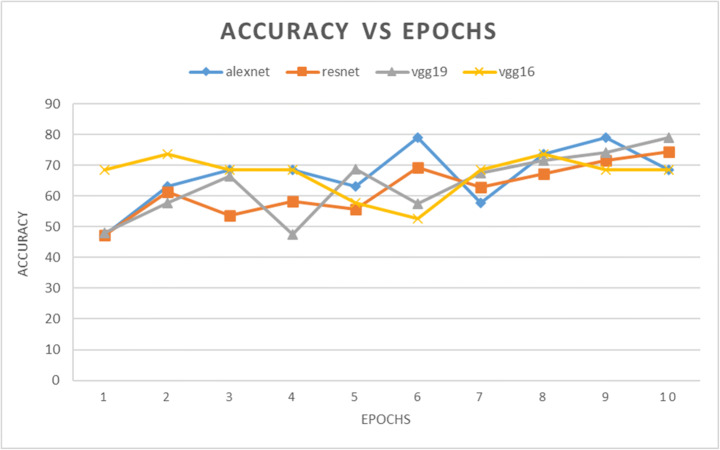
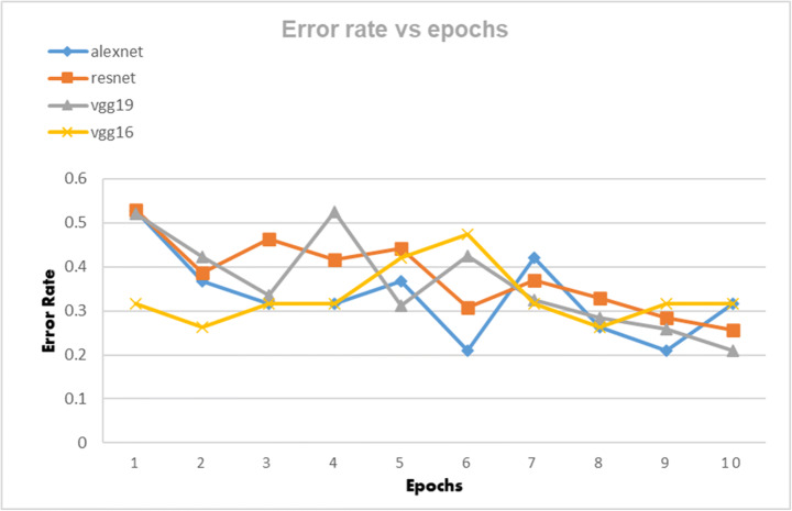
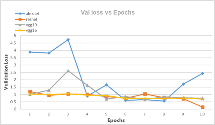
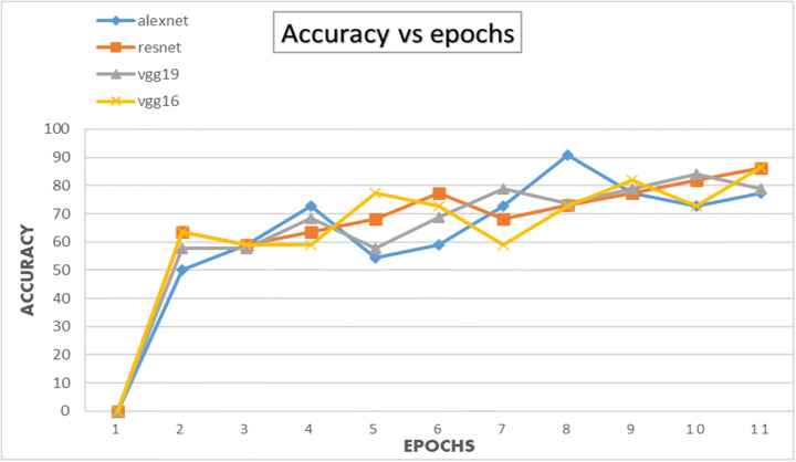
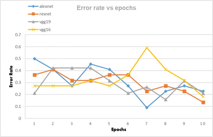
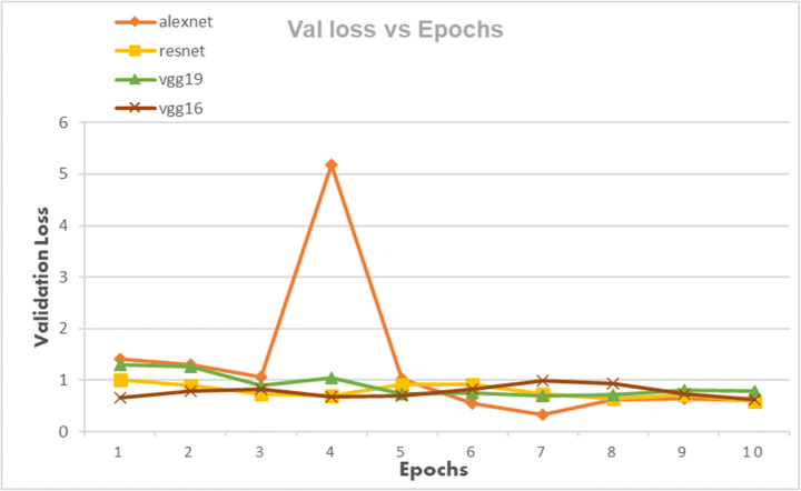
The CNN architectures were loaded from the Fastai library using the cnn_learner function. The CNN architectures are data-thirsty networks and we have only 381 knee x-ray scans having 60 in normal, 245 in osteopenia, and 76 in osteoporosis class so to increase the number of images data augmentation was done by using the Dataloader() function from Fastai library. The CNN networks were first trained on just our dataset and then transfer learning was employed by using the pretrained networks trained on ImageNet dataset containing millions of images to check whether transfer learning can improve the classification performance or not. Due to less number of images, the dataset was divided into a 95:5 ratio of training and validation sets. All four CNN architectures namely: AlexNet, ResNet-18, VggNet-16, and VggNet-19 were first only trained with the training set of knee x-ray images for 10 epochs and then CNNs pretrained with ImageNet dataset was trained with knee x-ray dataset. The performance of both types of CNNs was measured in terms of accuracy, error rate and validation loss which are shown in table form as well as graphically below. The Tables 3, 4 and 5 show the results obtained when CNNs were not pre-trained with ImageNet dataset and corresponding graphs are displayed in Figs. 4, 5 and 6 respectively. Results corresponding to pretrained CNNs are shown in Tables 6, 7 and 8 and graphically displayed in Figs. 7, 8 and 9.

Table 3.

The table depicts the error rates achieved by AlexNet, VggNet-19, ResNet, and VggNet-16 for 10 epochs

Model	Error Rate
	Loss_1	Loss_2	Loss_3	Loss_4	Loss_5	Loss_6	Loss_7	Loss_8	Loss_9	Loss_10
AlexNet	0.526316	0.368421	0.315789	0.315789	0.368421	0.210526	0.421053	0.263158	0.210526	0.315789
ResNet	0.5284	0.38748	0.464	0.41679	0.4428	0.3079	0.37	0.328	0.284	0.257
VggNet-19	0.5202	0.4222	0.3346	0.5252	0.3121	0.4251	0.3254	0.2841	0.2588	0.210526
VggNet-16	0.315789	0.263158	0.315789	0.315789	0.421053	0.473684	0.315789	0.263158	0.315789	0.315789

Table 4.

The table depicts the validation losses of AlexNet, VggNet-19, ResNet, and VggNet-16 for 10 epochs

Model	Validation Loss
	error-1	error-2	error-3	error-4	error-5	error-6	error-7	error-8	error-9	error-10
AlexNet	3.886485	3.811952	4.722492	0.888557	1.653029	0.596375	0.65505	0.544729	1.703589	2.444296
ResNet	1.199991	0.935812	1.044388	0.99777	0.864306	0.748894	1.044388	0.784841	0.71679	0.13829
VggNet-19	1.011665	1.292617	2.610984	1.623787	0.691115	0.857193	0.671244	0.840298	0.771979	0.747634
VggNet-16	1.016403	1.006614	1.040957	0.952533	0.92211	0.733812	0.740189	0.736071	0.758872	0.685425

Table 5.

The table depicts the accuracies of AlexNet, VggNet-19, ResNet, and VggNet-16 for 10 epochs

Model	Accuracy for 10 epochs
	Epoch-1	Epoch − 2	Epoch-3	Epoch − 4	Epoch − 5	Epoch − 6	Epoch − 7	Epoch − 8	Epoch − 9	Epoch − 10
AlexNet	47.37	63.16	68.42	68.42	63.16	78.95	57.89	73.68	78.95	68.42
ResNet	47.16	61.252	53.6	58.321	55.72	69.21	63	67.2	71.6	74.3
VggNet-19	47.98	57.78	66.54	47.48	68.79	57.49	67.46	71.59	74.12	78.9
VggNet-16	68.42	73.68	68.42	68.42	57.89	52.63	68.42	73.68	68.42	68.42

Fig. 4.

The classification accuracies for AlexNet, VggNet-19, ResNet, and VggNet-16 for 10 epochs

Fig. 5.

Error rate of AlexNet, VggNet-19, ResNet, and VggNet-16 achieved for 10 epochs

Fig. 6.

Validation Loss of AlexNet, VggNet-19, ResNet, and VggNet-16 achieved for 10 epochs

Table 6.

The table depicts the error rates achieved by AlexNet, VggNet-19, ResNet, and VggNet-16 for 10 epochs

Model	Error Rate
	Loss_1	Loss_2	Loss_3	Loss_4	Loss_5	Loss_6	Loss_7	Loss_8	Loss_9	Loss_10
AlexNet	0.5	0.409091	0.272727	0.454545	0.409091	0.272727	0.090909	0.227273	0.272727	0.227273
ResNet	0.363636	0.409091	0.318182	0.318182	0.363636	0.363636	0.227273	0.272727	0.227273	0.136364
VggNet-19	0.210526	0.421053	0.421053	0.421053	0.315789	0.210526	0.263158	0.157895	0.315789	0.210526
VggNet-16	0.272727	0.272727	0.272727	0.318182	0.272727	0.363636	0.590909	0.409091	0.318182	0.181818

Table 7.

The table depicts the validation losses of AlexNet, VggNet-19, ResNet, and VggNet-16 for 10 epochs

Model	Validation Loss
	error-1	error-2	error-3	error-4	error-5	error-6	error-7	error-8	error-9	error-10
AlexNet	1.417419	1.300952	1.068952	5.189301	1.026389	0.543029	0.325405	0.630233	0.639842	0.598446
ResNet	0.91028	0.91676	0.74584	0.70828	0.92563	0.9123	0.73799	0.641843	0.714709	0.59273
VggNet-19	1.33567	1.27235	0.954364	1.049802	0.741645	0.76157	0.69157	0.722578	0.81445	0.78148
VggNet-16	0.667435	0.790739	0.821053	0.678536	0.702504	0.820445	0.980566	0.92768	0.724928	0.625168

Table 8.

The table depicts the accuracies of AlexNet, VggNet-19, ResNet, and VggNet-16 for 10 epochs

Model	Accuracy for 10 epochs
	Epoch-1	Epoch − 2	Epoch-3	Epoch − 4	Epoch − 5	Epoch − 6	Epoch − 7	Epoch − 8	Epoch − 9	Epoch − 10
AlexNet	50	59.1	72.8	54.5	59.1	72.7	91.1	77.2	72.7	77.7
VggNet-16	63.6	59.9	59.9	77.2	72.7	59.9	72.7	81.8	72.7	86.3
ResNet	63.6	59	63.6	68.1	77.2	68.1	73	77.2	81.8	86.3
VggNet-19	57.8	57.8	68.4	57.8	68.9	78.9	73.6	78.9	84.2	78.9

Bold text inside the body is to highlight the highest accuracy achieved by each classifier

Fig. 7.

The classification accuracies for AlexNet, VggNet-19, ResNet, and VggNet-16 for 10 epochs

Fig. 8.

Error rate of AlexNet, VggNet-19, ResNet, and VggNet-16 achieved for 10 epochs

Fig. 9.

Validation Loss of AlexNet, VggNet-19, ResNet, and VggNet-16 achieved for 10 epochs

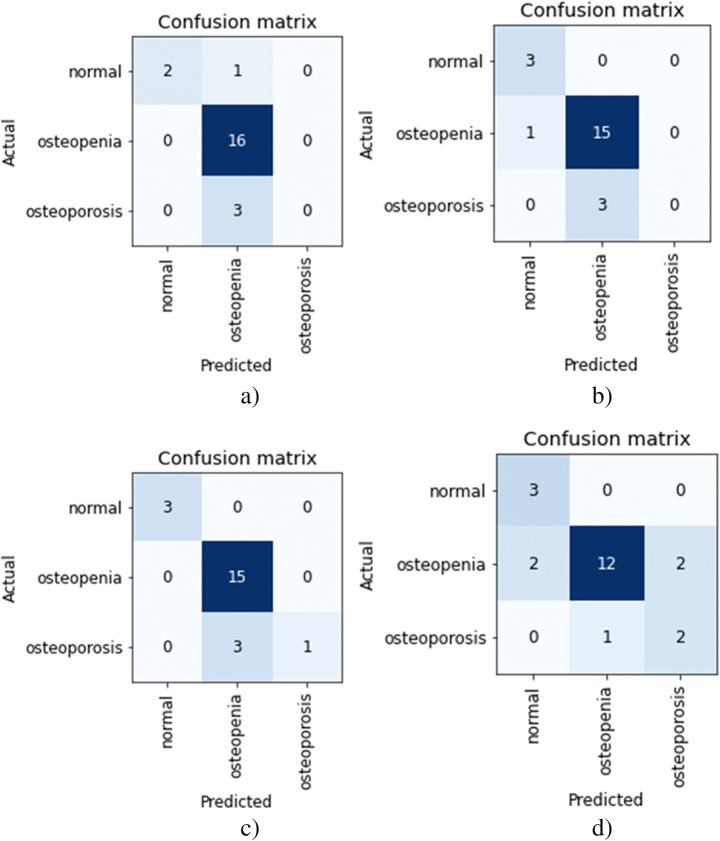
Figure 10 shows the confusion matrix for AlexNet, ResNet, Vgg-19, and Vgg-16 models obtained for validation sets in pretrained CNNs. The osteopenia disease group has the highest classification accuracy with X-ray images. The images with the lowest classification accuracy are the osteoporosis images. Both the variants of VggNet CNN were not able to classify the osteoporotic images while obtaining the highest accuracy of 86.3 and 84.2 for Vgg-16 and Vgg-19 respectively. The poor classification performance for classifying the osteoporosis disease group and then the normal group is because the number of images in each class was low. The collected dataset of knee X-ray images had a maximum number of images in the osteopenia group than the normal and osteoporosis group. The results from all CNN architectures suggest that X-ray images can be used to detect osteoporosis from the knees.

Fig. 10.

The confusion matrixes for the validation set of the dataset, (a) Vgg-19, (b) Vgg-16, (c) ResNet, (d) AlexNet

Discussion

This is the first study that is aimed to detect osteoporosis from knee X-rays that are classified into disease groups (osteopenia and osteoporosis) and normal on basis of BMD values obtained from the medical diagnostic test QUS. We have used the power of CNN networks to classify the class of X-ray images by interpreting the differences in the image groups and then classifying them automatically. The performance of well-known CNNs was compared in order to get the best performing CNN for detecting osteoporosis from knee X-rays. The participants of the study included participants of all genders and ages. Deep learning architectures have been used to detect osteoporosis from other sites like hand, spine, or hip scans.

From Figs. 4 and 7 we can observe that the best classification accuracy is achieved by AlexNet and the lowest performance is obtained by Vgg-19 and Vgg-16 in normal CNN and pre trained CNN respectively. In Table 9 we have summarised the best values from all the metrics of both types of CNNs. We can see that the best classification accuracy achieved by AlexNet, ResNet, VggNet-16, and VggNet-19 is 78.95%, 74.3%, 78.9%, and 73.68% and 91%, 86.4%, 86.3%, and 84.2% for normal CNN and pretrained CNN respectively. From Table 9, we can see that the lowest error rates achieved by AlexNet, ResNet, VggNet-16, and VggNet-19 are 0.21, 0.257, 0.21, and 0.263, and 0.09, 0.136, 0.181, and 0.157 for normal CNN and pretrained CNN respectively. Also we can see that the lowest validation loss from AlexNet, ResNet, VggNet-16, and VggNet-19 is 0.544, 0.138, 0.671 and 0.685 and 0.325, 0.694, 0.625, and 0.692 for normal and pretrained CNN respectively. The results obtained suggests that when CNNs were trained with only knee x-ray dataset although showed good classification accuracy but pretrained CNNs when trained with knee x-ray dataset showed improved accuracy. This implies that using transfer learning improves the overall performance of the system without building a new CNN from scratch or adding or deleting any layer. The highest classification accuracy of 91% achieved by AlexNet suggests of using CNN for classification of knee X-ray images. The previous deep learning models used in osteoporosis detection from other sites showed good performance but had some limitations for eg; in study of Zhang et al. [71] to detect osteoporosis from lumbar spine X-rays using deep learning model but they included that dataset containing the images of only women aged ≥50. Lee et al. [36] achieved the maximum classification accuracy of 71% with VGG for feature extraction and random forest for classification. Yasaka et al. [68] studied CT images of vertebrae and found a good correlation between the predicted BMD from CNN and the DXA BMD. Study of Liu et al. [40] poorly diagnosed the images of the bone mass reduction group and osteoporosis group. AlexNet CNN used by Yu et al. [70] detected osteoporosis from DPRs with good accuracy but doesn’t include the osteopenia class exclusively. He et al. [24] analysed that radiographic parameters from knee X-rays have a significant correlation with BMD and T-score. Bortone et al. [5] used the artificial neural network and support vector machine classifiers to classify the subjects with osteopenia, osteoporosis and normal bone functions on basis of the lifestyle factors, the previous history of fractures based on data, collected from participants by filling up the questionaries. Tang et al. [57] used CNN model for bone type determination with accuracy of 76.65%. Table 10 presents the comparison of our work with existing state-of-the-art works.

Table 9.

Comparison of different metrics of normal CNN and pretrained CNN

	Normal CNN			Pre-trained CNN
Model	Accuracy	Error rate	Validation Loss	Accuracy	Error rate	Validation Loss
AlexNet	78.95	0.21	0.544	90.91	0.09	0.54
ResNet	74.3	0.257	0.138	86.3	0.136	0.592
VggNet-19	78.9	0.21	0.671	84.2	0.157	0.691
VggNet-16	73.68	0.263	0.685	86.3	0.181	0.625

Table 10.

Comparison with existing state-of-the-art works

Author	Year	Bone Type	Image Type	Classifier	Performance
			Computed		TPR: 64.7%
Hatano et al	2016	Phalanges	Radiography	DCNN	FPR: 6.51%
			Computed
Tomita et al	2018	Vertebrae	Tomography	LSTM	acc: 89.2%
Lee et al	2018	tooth	Radiographs	DCNN	AUC: 0.9991
Derkatch et al	2019	Vertebrae	DXA	CNN	AUC:0.94
Tecle et al	2020	Hand	Radiographs	LeNet	acc: 99.62%,
Lee et al	2020	Tooth lumbar	Radiographs	Vgg-16	AUC: 0.858
Zhang et al	2020	spine	X-ray	DCNN	AUC: 0.81
	2021		Computed
Fang et al		Vertebrae	Tomography	DenseNet-121	r: 0.98
			Computed
Sollmann et al	2022	Spine	Tomography	DCNN	AUC: 0.862
Sukegawa et al	2022	DPRs	Radiographs	Ensemble CNN	acc: 84%
Pretrained CNN1		Knee	X-ray	AlexNet	91%
Pretrained CNN2		Knee	X-ray	VggNet-16	86.30%
Pretrained CNN3		Knee	X-ray	ResNet	86.30%
Pretrained CNN4		Knee	X-ray	VggNet-19	84.20%

Our dataset consists of image data as well as numerical data containing the clinical, lifestyle, and other important factors. But in this study, we devised a system that can detect osteoporosis directly from X-ray images. The images used are grouped in three different classes viz.: normal, osteopenia, and osteoporosis on basis of the T-score calculated from the QUS system, unlike many other computer-aided systems which are built on binary classification. The images consist of the x-rays from both males and females and the age group varies from 18 to 107 years of age. The deep learning-based detection system for osteoporosis can be a good choice and can help medical experts to identify the patients with risk of osteoporosis and osteoporotic risk fractures at very early stages. The deep learning model trained on the supervised X-ray images can help in diagnosing osteoporosis not only in the early stages but also can prove to be a cost-effective and easily available tool in low-income economies having higher population rates like India or other countries. The clinical factors can also help the medical practitioner to make a wise decision for a patient in addition to classification from a deep learning system. The CNN systems are completely automatic as they do not require any additional effort for feature extraction, selection, or classification. The inability of the VggNets to classify the osteoporotic class can be the result of having fewer images in this class. The maximum participants were diagnosed with osteopenia from the QUS system and all four CNNs were able to detect the Knee X-rays of osteopenia class very efficiently. We could increase the efficiency of CNNs in classifying the normal and osteoporotic x-rays by adding more images to each class. The main outcomes of our study are summarised below:

1. Mostly the studies work on a particular age group or gender. The X-ray images included in the study are collected from different age groups and all genders.

2. Our study covers all three classification criteria of osteoporosis i.e.; normal, osteopenia, and osteoporosis. and our study is validated by the medical test QUS which calculates the T-score by measuring the bone mineral density of the bones.

3. Classification of x-rays with CNN is purely automatic. It doesn’t involve separate methodologies for feature extraction, selection, or classification.

4. We have compared the performance of well-known CNN architectures viz.: AlexNet, VggNet-16, VggNet-19, and ResNet-18 in classifying the knee X-rays.

5. To overcome the problem of the small number of images in the dataset we have used data augmentation and transfer learning.

6. The comparison with existing state-of-the-art works shows that our proposed model shows good performance (Table 10) and can be used for osteoporosis detection.

Our study suffers from some limitations. Firstly the performance of the CNNs was affected by a small number of images in the dataset especially in normal and osteoporosis classes. We believe increasing the number of images in each class will enhance the performance of the networks. Secondly, the T-score was calculated from the QUS system which is a cost-effective technique for assessing the fracture risk by examining the calcaneus of the different bones but it gives unstable bone parameters and its validation database is different from the BMD DXA. So, we can further validate our dataset by measuring the BMD with DXA. Thirdly, the clinical and other factors which were collected from the participants can also help in predicting the bone condition of the patient but it was not used in the classification process. So, we will try to inculcate these features with image data for better diagnosis. Despite some limitations our comparison could help to find the best CNN architecture to be used in clinical settings for diagnosing osteoporosis at early stages, reducing the risk of fractures which will automatically decrease the testing and treatment costs of osteoporosis.

We can summarize that the simple knee X-ray scans, taken for whatsoever reason can be passed through the system made with CNN and can be assessed for risk of osteoporosis or osteopenia without any extra cost or screening. The medical acceptance of these deep learning systems is not yet available but using Artificial Intelligent systems to give the first advice on the possibility of having some disease can be very helpful in modern medicine.

Conclusion and recommendation

In our study, we have evaluated and compared the performance of popular CNN architectures namely ResNet-18, VggNet-16, AlexNet, and VggNet-19 in diagnosing osteoporosis from knee X-ray images. The X-ray images used were taken from the custom dataset that was classified into normal, osteopenia, and osteoporosis group with the help of a medically accepted BMD test known as the Quantitative Ultrasound system which calculates the T-score by measuring the BMD of bone. The custom dataset contained a total of 381 knee x-ray scans. The results show that the best performance was achieved by AlexNet with 91% of accuracy and the lowest performance of 84.2% was given by VggNet-19. The results from all CNNs showed good diagnostic performance and suggest that diagnosing osteoporosis from knee X-ray using transfer learning with CNN can serve to be a cost-effective and readily available diagnostic tool.

In the future, more data can be collected especially from normal and osteoporotic subjects. Secondly, we can find the relationship of knee osteoporosis with osteoporosis at other sites to make universal diagnostic system of osteoporosis. Thirdly, the system can be build which will detect osteoporosis from clinical factors in combination with images.

Data availability

The image data that support the findings of this study are available in “Knee X-ray Osteoporosis Database” with the identifier “https://data.mendeley.com/datasets/fxjm8fb6mw/10.17632/fxjm8fb6mw.2” [43].

Declarations

Conflict of interest

The authors declare that they have no conflict of interest.

References

- 1.Ali AM, El-Shafie M, Willett KM. Failure of fixation of tibial plateau fractures. J Orthop Trauma. 2002;16(5):323–329. doi: 10.1097/00005131-200205000-00006. [DOI] [PubMed] [Google Scholar]
- 2.Ambati LS, El-Gayar O. Human activity recognition: a comparison of machine learning approaches. J Midwest Assoc Inf Syst (JMWAIS) 2021;2021(1):4. [Google Scholar]
- 3.Ambati LS, El-Gayar OF, Nawar N (2021) "Design principles for multiple sclerosis Mobile self-management applications: a patient-centric perspective," in AMCIS
- 4.Becker DJ, Kilgore ML, Morrisey MA (2010) "The societal burden of osteoporosis," vol. 12, no. 3, pp. 186–191 [DOI] [PubMed]
- 5.Bortone I, Trotta GF, Cascarano GD, Paola R, Antonio B, De Feudis I, Buongiorno D, Loconsole C, Bevilacqua V (2018) A supervised approach to classify the status of bone mineral density in post-menopausal women through static and dynamic baropodometry. In: 2018 International Joint Conference on Neural Networks (IJCNN). IEEE, pp 1–7
- 6.Brett AD, Brown JK. Quantitative computed tomography and opportunistic bone density screening by dual use of computed tomography scans. J Orthop Transl. 2015;3(4):178–184. doi: 10.1016/j.jot.2015.08.006. [DOI] [PMC free article] [PubMed] [Google Scholar]
- 7.Chen Y, Guo Y, Zhang X, Mei Y, Feng Y, Zhang XJER. Bone susceptibility mapping with MRI is an alternative and reliable biomarker of osteoporosis in postmenopausal women. Eur Radiol. 2018;28(12):5027–5034. doi: 10.1007/s00330-018-5419-x. [DOI] [PubMed] [Google Scholar]
- 8.Chen Y, Zhang Q, Wu Y, Liu B, Wang M, Lin Y (2018) Fine-tuning ResNet for breast cancer classification from mammography. In: The International Conference on Healthcare Science and Engineering. Springer, pp 83–96
- 9.C. Cooper, L. J. J. T. i. E. Melton III, and Metabolism, "Epidemiology of osteoporosis," vol. 3, no. 6, pp. 224–229, 1992. [DOI] [PubMed]
- 10.Court-Brown CM, Caesar BJI. Epidemiology of adult fractures: a review. Injury. 2006;37(8):691–697. doi: 10.1016/j.injury.2006.04.130. [DOI] [PubMed] [Google Scholar]
- 11.Deniz CM, et al. Segmentation of the proximal femur from MR images using deep convolutional neural networks. Sci Rep. 2018;8(1):1–14. doi: 10.1038/s41598-018-34817-6. [DOI] [PMC free article] [PubMed] [Google Scholar]
- 12.Derkatch S, Kirby C, Kimelman D, Jozani MJ, Davidson JM, Leslie WDJR. Identification of vertebral fractures by convolutional neural networks to predict nonvertebral and hip fractures: a registry-based cohort study of dual X-ray absorptiometry. Radiol. 2019;293(2):405–411. doi: 10.1148/radiol.2019190201. [DOI] [PubMed] [Google Scholar]
- 13.Dimai HPJB (2017) "Use of dual-energy X-ray absorptiometry (DXA) for diagnosis and fracture risk assessment; WHO-criteria, T-and Z-score, and reference databases," vol. 104, pp. 39–43 [DOI] [PubMed]
- 14.Ebrahimi-Ghahnavieh A, Luo S, Chiong R (2019) Transfer learning for Alzheimer's disease detection on MRI images. In: 2019 IEEE International Conference on Industry 4.0, Artificial Intelligence, and Communications Technology (IAICT). IEEE, pp 133–138
- 15.El-Gayar OF, Ambati LS, Nawar N (2020) "Wearables, artificial intelligence, and the future of healthcare," in AI and Big Data’s Potential for Disruptive Innovation: IGI Global, pp. 104–129
- 16.Fang Y, et al. Opportunistic osteoporosis screening in multi-detector CT images using deep convolutional neural networks. Eur Radiol. 2021;31(4):1831–1842. doi: 10.1007/s00330-020-07312-8. [DOI] [PubMed] [Google Scholar]
- 17.Fathima SN, Tamilselvi R, Beham MPJB, Journal P. XSITRAY: a database for the detection of osteoporosis condition. Biomed Pharma J. 2019;12(1):267–271. doi: 10.13005/bpj/1637. [DOI] [Google Scholar]
- 18.Ferizi U, et al. Artificial intelligence applied to osteoporosis: a performance comparison of machine learning algorithms in predicting fragility fractures from MRI data. J Magn Reson Imaging. 2019;49(4):1029–1038. doi: 10.1002/jmri.26280. [DOI] [PMC free article] [PubMed] [Google Scholar]
- 19.Gregg EW et al. (1997) "The epidemiology of quantitative ultrasound: a review of the relationships with bone mass, osteoporosis and fracture risk," vol. 7, no. 2, pp. 89–99 [DOI] [PubMed]
- 20.Guo M, Du Y (2019) "Classification of Thyroid Ultrasound Standard Plane Images using ResNet-18 Networks," in 2019 IEEE 13th International Conference on Anti-counterfeiting, Security, and Identification (ASID), pp. 324–328: IEEE
- 21.Hans D, Baim S. Quantitative ultrasound (QUS) in the management of osteoporosis and assessment of fracture risk. J Clin Densitometry. 2017;20(3):322–333. doi: 10.1016/j.jocd.2017.06.018. [DOI] [PubMed] [Google Scholar]
- 22.Hatano K, Murakami S, Lu H, Tan JK, Kim H, Aoki T (2017) Classification of osteoporosis from phalanges CR images based on DCNN. In: 2017 17th International Conference on Control, Automation and Systems (ICCAS). IEEE, pp 1593–1596
- 23.He K, Zhang X, Ren S, Sun J (2016) "Deep residual learning for image recognition," in Proceedings of the IEEE conference on computer vision and pattern recognition, pp. 770–778
- 24.He Q, et al. Radiographic predictors for bone mineral loss: cortical thickness and index of the distal femur. Bone Joint Res. 2018;7(7):468–475. doi: 10.1302/2046-3758.77.BJR-2017-0332.R1. [DOI] [PMC free article] [PubMed] [Google Scholar]
- 25.Hosny KM, Kassem MA, Foaud MM. Classification of skin lesions using transfer learning and augmentation with Alex-net. Plos One. 2019;14(5):e0217293. doi: 10.1371/journal.pone.0217293. [DOI] [PMC free article] [PubMed] [Google Scholar]
- 26.Howard J, Gugger S (2020) Fastai: A layered API for deep learning. J Information 11(2):108
- 27.Jain S, Salau AO. An image feature selection approach for dimensionality reduction based on kNN and SVM for AkT proteins. Cogent Eng. 2019;6(1):1599537. doi: 10.1080/23311916.2019.1599537. [DOI] [Google Scholar]
- 28.Jiang H, Yates CJ, Gorelik A, Kale A, Song Q, Wark JD. Peripheral Quantitative Computed Tomography (pQCT) measures contribute to the understanding of bone fragility in older patients with low-trauma fracture. J Clin Densitom. 2018;21(1):140–147. doi: 10.1016/j.jocd.2017.02.003. [DOI] [PubMed] [Google Scholar]
- 29.Johnell O, Kanis JJOI (2006) "An estimate of the worldwide prevalence and disability associated with osteoporotic fractures," vol. 17, no. 12, pp. 1726–1733 [DOI] [PubMed]
- 30.Kanis JA (2008) "Assessment of osteoporosis at the primary health-care level. Techn Rep,"
- 31.Khan Z, et al. Diabetic Retinopathy Detection Using VGG-NIN a Deep Learning Architecture. IEEE Access. 2021;9:61408–61416. doi: 10.1109/ACCESS.2021.3074422. [DOI] [Google Scholar]
- 32.Krishnaraj A, et al. Simulating dual-energy X-ray absorptiometry in CT using deep-learning segmentation cascade. J Am College Radiol. 2019;16(10):1473–1479. doi: 10.1016/j.jacr.2019.02.033. [DOI] [PubMed] [Google Scholar]
- 33.Krizhevsky A, Sutskever I, Hinton GE. Imagenet classification with deep convolutional neural networks. Commun ACM. 2012;25:1097–1105. [Google Scholar]
- 34.LeCun Y, Bottou L, Bengio Y, Haffner P (1998) Gradient-based learning applied to document recognition. J Proceedings of the IEEE 86(11):2278–2324
- 35.Lee J-S, Adhikari S, Liu L, Jeong H-G, Kim H, Yoon S-J. Osteoporosis detection in panoramic radiographs using a deep convolutional neural network-based computer-assisted diagnosis system: a preliminary study. Dentomaxillofacial Radiol. 2019;48(1):20170344. doi: 10.1259/dmfr.20170344. [DOI] [PMC free article] [PubMed] [Google Scholar]
- 36.Lee S, Choe EK, Kang HY, Yoon JW, Kim HS. The exploration of feature extraction and machine learning for predicting bone density from simple spine X-ray images in a Korean population. Skelet Radiol. 2020;49(4):613–618. doi: 10.1007/s00256-019-03342-6. [DOI] [PubMed] [Google Scholar]
- 37.Lee K-S, Jung S-K, Ryu J-J, Shin S-W, Choi J. Evaluation of transfer learning with deep convolutional neural networks for screening osteoporosis in dental panoramic radiographs. J Clin Med. 2020;9(2):392. doi: 10.3390/jcm9020392. [DOI] [PMC free article] [PubMed] [Google Scholar]
- 38.Li Q, Cai W, Wang X, Zhou Y, Feng DD, Chen M (2014) "Medical image classification with convolutional neural network," in 2014 13th international conference on control automation robotics & vision (ICARCV), pp. 844–848: IEEE
- 39.Liu D, Liu Y, Dong L (2019) "G-ResNet: Improved ResNet for brain tumor classification," in International Conference on Neural Information Processing, pp. 535–545: Springer
- 40.Liu J, Wang J, Ruan W, Lin C, Chen D. Diagnostic and Gradation Model of Osteoporosis Based on Improved Deep U-Net Network. J Med Syst. 2020;44(1):15. doi: 10.1007/s10916-019-1502-3. [DOI] [PubMed] [Google Scholar]
- 41.Lu S, Wang S-H, Zhang Y-DJH. Detecting pathological brain via ResNet and randomized neural networks. Heliyon. 2020;6(12):e05625. doi: 10.1016/j.heliyon.2020.e05625. [DOI] [PMC free article] [PubMed] [Google Scholar]
- 42.Lu S, Wang S-H, Zhang Y-D, Applications (2020) "Detection of abnormal brain in MRI via improved AlexNet and ELM optimized by chaotic bat algorithm," pp. 1–13
- 43.Majeed Wani I, Sakshi A (2021) Knee X-ray Osteoporosis Database. Mendeley Data V2. 10.17632/fxjm8fb6mw.2
- 44.Mallina R, Kanakaris NK, Giannoudis PV. Peri-articular fractures of the knee: an update on current issues. The Knee. 2010;17(3):181–186. doi: 10.1016/j.knee.2009.10.011. [DOI] [PubMed] [Google Scholar]
- 45.Militante SV (2019) "Malaria Disease Recognition through Adaptive Deep Learning Models of Convolutional Neural Network," in 2019 IEEE 6th International Conference on Engineering Technologies and Applied Sciences (ICETAS), pp. 1–6: IEEE
- 46.Mithal A, Bansal B, Kyer CS, Ebeling P, metabolism The Asia-pacific regional audit-epidemiology, costs, and burden of osteoporosis in India 2013: a report of international osteoporosis foundation. Indian J Endocrinol. 2014;18(4):449. doi: 10.4103/2230-8210.137485. [DOI] [PMC free article] [PubMed] [Google Scholar]
- 47.Rahman T, Chowdhury MEH, Khandakar A, Islam KR, Islam KF, Mahbub ZB, Kadir MA, Kashem S (2020) Transfer learning with deep convolutional neural network (CNN) for pneumonia detection using chest X-ray. J Appl Sci 10(9):3233
- 48.Salau AO, Jain S. Adaptive diagnostic machine learning technique for classification of cell decisions for AKT protein. Inf Med Unlocked. 2021;23:100511. doi: 10.1016/j.imu.2021.100511. [DOI] [Google Scholar]
- 49.Salau AO, Jain S, Biotechnology Computational modeling and experimental analysis for the diagnosis of cell survival/death for Akt protein. J Gen Eng Biotechnol. 2020;18(1):1–10. doi: 10.1186/s43141-020-00026-w. [DOI] [PMC free article] [PubMed] [Google Scholar]
- 50.Salih SQ, Abdulla HKh, Ahmed ZSh, Surameery NMS, Rashid RDh (2020) Modified alexnet convolution neural network for covid-19 detection using chest x-ray images, pp 119–130
- 51.Simonyan K, Zisserman A (2014) "Very deep convolutional networks for large-scale image recognition,"
- 52.Sollmann N et al. (2022) "Automated opportunistic osteoporosis screening in routine computed tomography of the spine–comparison with dedicated quantitative CT," [DOI] [PubMed]
- 53.Stange R, Raschke MJ (2020) Principles, and Practice, "Osteoporotic distal femoral fractures When to replace and how,"
- 54.Sukegawa S, et al. Identification of osteoporosis using ensemble deep learning model with panoramic radiographs and clinical covariates. Sci Rep. 2022;12(1):1–10. doi: 10.1038/s41598-022-10150-x. [DOI] [PMC free article] [PubMed] [Google Scholar]
- 55.Suzuki K, Technology Overview of deep learning in medical imaging. Radiol Phys Technol. 2017;10(3):257–273. doi: 10.1007/s12194-017-0406-5. [DOI] [PubMed] [Google Scholar]
- 56.Szegedy C, Liu W, Jia Y, Sermanet P, Reed S, Anguelov D, Erhan D, Vanhoucke V, Rabinovich A (2015) Going deeper with convolutions. In: Proceedings of the IEEE conference on computer vision and pattern recognition, pp 1–9
- 57.Tang C et al. (2019) "CNN-based automatic detection of bone conditions via diagnostic CT images for osteoporosis screening,"
- 58.Tecle N, Teitel J, Morris MR, Sani N, Mitten D, Hammert WC. Convolutional neural network for second metacarpal radiographic osteoporosis screening. J Hand Surge. 2020;45(3):175–181. doi: 10.1016/j.jhsa.2019.11.019. [DOI] [PubMed] [Google Scholar]
- 59.Tomita N, Cheung YY, Hassanpour S, Medicine Deep neural networks for automatic detection of osteoporotic vertebral fractures on CT scans. Comput Biol Med. 2018;98:8–15. doi: 10.1016/j.compbiomed.2018.05.011. [DOI] [PubMed] [Google Scholar]
- 60.Torrey L, Shavlik J (2010) "Transfer learning," in Handbook of research on machine learning applications and trends: algorithms, methods, and techniques: IGI global, pp. 242–264
- 61.Wang S-P, Wu P-K, Lee C-H, Shih C-M, Chiu Y-C, Hsu C-E. Association of osteoporosis and varus inclination of the tibial plateau in postmenopausal women with advanced osteoarthritis of the knee. BMC Musculoskelet Disord. 2021;22(1):1–8. doi: 10.1186/s12891-021-04090-2. [DOI] [PMC free article] [PubMed] [Google Scholar]
- 62.Wani IM, Arora S (2020) Deep neural networks for diagnosis of osteoporosis: a Review. In: Proceedings of ICRIC 2019. Springer, pp 65–78
- 63.Wani IM, Arora S. Computer-aided diagnosis systems for osteoporosis detection: a comprehensive survey. Med Biol Eng Comput. 2020;58(9):1873–1917. doi: 10.1007/s11517-020-02171-3. [DOI] [PubMed] [Google Scholar]
- 64.Wani IM, Arora S (2021) A knee X-ray database for osteoporosis detection. In: 2021 9th International Conference on Reliability, Infocom Technologies and Optimization (Trends and Future Directions)(ICRITO). IEEE, pp 1–5
- 65.World Health Organization (1994) Assessment of fracture risk and its application to screening for postmenopausal osteoporosis: report of a WHO study group [meeting held in Rome from 22 to 25 June 1992] [PubMed]
- 66.Yadav SS, Jadhav SM. Deep convolutional neural network based medical image classification for disease diagnosis. J Big Data. 2019;6(1):1–18. doi: 10.1186/s40537-019-0276-2. [DOI] [Google Scholar]
- 67.Yamamoto N, et al. Deep learning for osteoporosis classification using hip radiographs and patient clinical covariates. Biomolecules. 2020;10(11):1534. doi: 10.3390/biom10111534. [DOI] [PMC free article] [PubMed] [Google Scholar]
- 68.Yasaka K, Akai H, Kunimatsu A, Kiryu S, Abe O (2020) Prediction of bone mineral density from computed tomography: application of deep learning with a convolutional neural network. J Eur Radiol: 1–9. 10.1007/s00330-020-06677-0 [DOI] [PubMed]
- 69.Yu X, Wang S-H. Abnormality diagnosis in mammograms by transfer learning based on ResNet18. Fundamenta Informaticae. 2019;168(2–4):219–230. doi: 10.3233/FI-2019-1829. [DOI] [Google Scholar]
- 70.Yu S, Chu P, Yang J, Huang B, Yang F, Megalooikonomou V, Ling H (2019) Multitask osteoporosis prescreening using dental panoramic radiographs with feature learning. J Smart Health
- 71.Zhang B, Yu K, Ning Z, Wang K, Dong Y, Liu X, Liu S, Wang J, Zhu C, Yu Q (2020) Deep learning of lumbar spine X-ray for osteopenia and osteoporosis screening: a multicenter retrospective cohort study. J Bone 140:115561 [DOI] [PubMed]
Associated Data
This section collects any data citations, data availability statements, or supplementary materials included in this article.
Data Availability Statement