Using Machine Learning to Identify Organ System Specific Limitations to Exercise Via Cardiopulmonary Exercise Testing

Abstract

Cardiopulmonary Exercise Testing (CPET) is a unique physiologic medical test used to evaluate human response to progressive maximal exercise stress. Depending on the degree and type of deviation from the normal physiologic response, CPET can help identify a patient’s specific limitations to exercise to guide clinical care without the need for other expensive and invasive diagnostic tests. However, given the amount and complexity of data obtained from CPET, interpretation and visualization of test results is challenging. CPET data currently require dedicated training and significant experience for proper clinician interpretation. To make CPET more accessible to clinicians, we investigated a simplified data interpretation and visualization tool using machine learning algorithms. The visualization shows three types of limitations (cardiac, pulmonary and others); values are defined based on the results of three independent random forest classifiers. To display the models’ scores and make them interpretable to the clinicians, an interactive dashboard with the scores and interpretability plots was developed. This machine learning platform has the potential to augment existing diagnostic procedures and provide a tool to make CPET more accessible to clinicians.

I. Introduction

Cardiopulmonary Exercise Testing (CPET) is a unique physiologically-based test for the assessment of human limitations to exercise through gas exchange analysis (i.e., O₂ and CO₂) via progressive maximal aerobic exercise [1]. Among its many uses in clinical medicine (e.g., diagnosis and prognosis of patients with cardiopulmonary disorders and those undergoing heart transplant) [2–4], CPET is used to identify impairments in individual body systems critical in sustaining the work of exercise: the lungs, heart, circulatory system, and skeletal muscle O₂-CO₂ exchange and mitochondrial metabolism [5]. Through simultaneous study of the responses of cardiovascular, pulmonary, peripheral vascular, and peripheral metabolic systems during exercise, CPET is a cost-effective and efficient diagnostic tool. It is capable of identifying and localizing primary functional limitations to exercise in a variety of disorders, i.e., myocardial ischemia, chronic obstructive pulmonary disease, or metabolic myopathies [6]. CPET is underutilized primarily due to the challenges of data interpretation, despite its advantages compared to more expensive and invasive testing to assess exertional dyspnea or exercise intolerance [1, 7].

Interpretation of CPET results for the purpose of identifying body system limitations in exercise requires incorporation of both maximal and submaximal data values into flowchart and graphical visualizations. One common method used to visualize and interpret CPET data is the Wasserman nine-panel plot (Figure 1), which takes advantage of the breadth and diversity of CPET data to display it in a format accessible to trained and experienced clinicians [8]. Even with the richness of data insights provided by platforms like the Wasserman nine-panel plot, however, correct CPET interpretation still requires many hours of specialized medical training and experience. Thus, CPET interpretation remains allusive to the less experienced reader, and different methods are needed to expand its use within the broader medical community [7].

Figure 1.

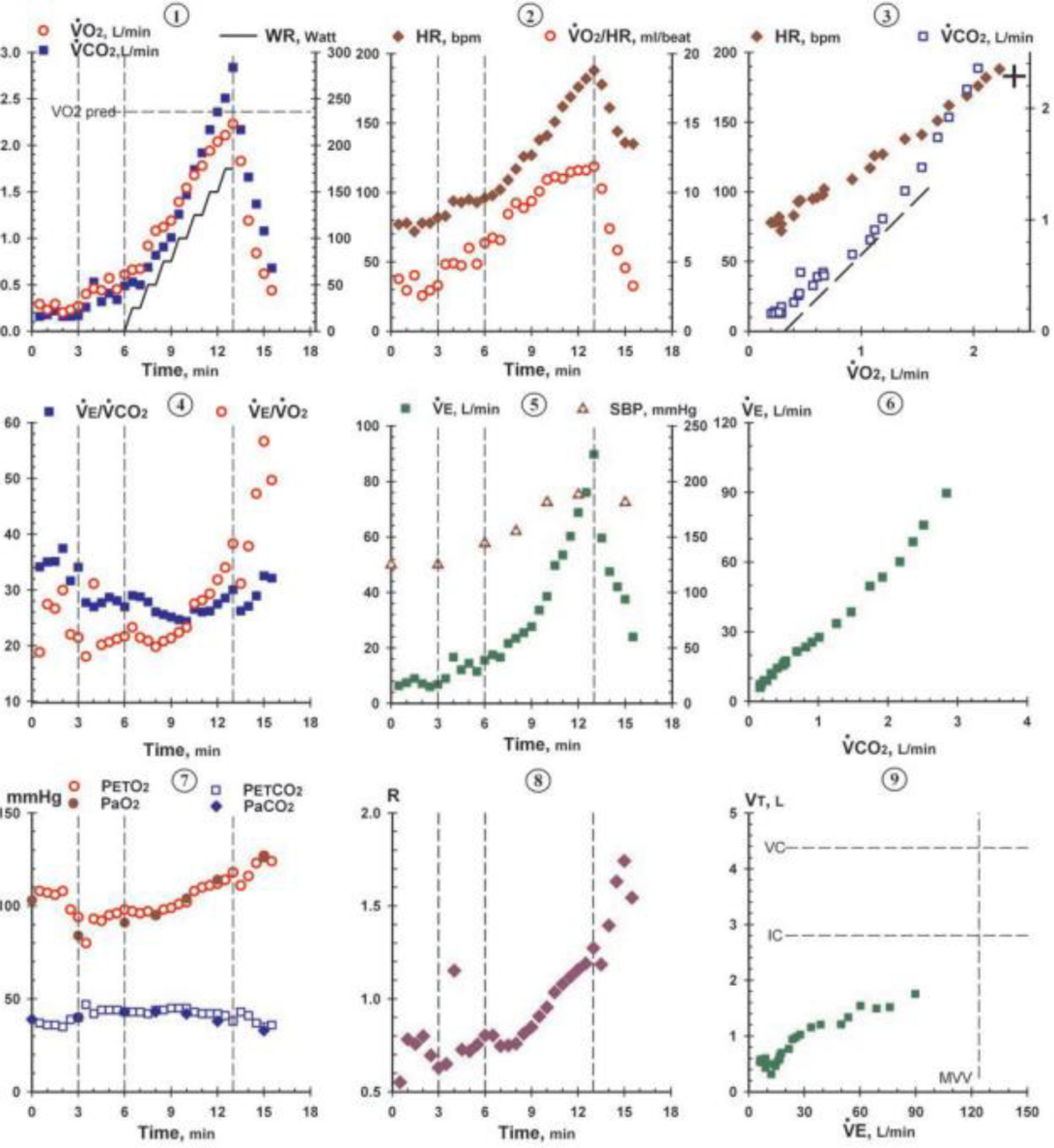
Example of Wasserman nine-panel plot (used with permission from Wolters Kluwer Health) [1].

To overcome barriers to CPET data interpretation, several solutions have been proposed to improve its utilization. Early attempts include changes to the scaling, styling the graphs, and standardizing the plots [8]. Another visualization alternative used changes in data variable relationships to classify severity in patients with heart failure [7]. In a preliminary proof-of-concept study, our team previously used simple formulas from CPET-generated data to assess and present organ system-specific limitations to exercise using both 2D and 3D plot visualizations [9]. CPET results from this preliminary work are presented as pulmonary, cardiac, and skeletal muscle limitations in percentages from 0% to 100%[9].

Machine learning algorithms hold considerable promise to simulate human analysis of CPET-generated data [10–13]. Machine learning methods use data engineering to identify key features from raw data and involve algorithms such as logistic regression, decision trees, time warping, and k-nearest neighbor matching [12, 14, 15]. Previous machine learning methods for CPET analysis used convolutional neural networks and recurrent neural networks to detect nonlinear patterns to determine the ventilatory threshold [12, 13]. Another study used data from CPET and support vector machine learning to differentiate patients with chronic heart failure (CHF) versus those with chronic obstructive pulmonary disease (COPD) [15].

In this study machine learning algorithms were applied to CPET-generated data for the purpose of identifying and differentiating among pulmonary, cardiac, and other system limitations to exercise and to aid clinical evaluation of exercise intolerance. Compared to previous studies, the model selection was done through the use of automatic machine learning.

II. METHODS

A. Data Collection and Labeling

Data from 225 CPET cases were used for analyses: 110 CPET cases obtained for the purposes of clinical assessment or for research purposes (from Duke University and the University of Virginia) and 115 cases used and transcribed from “Principles of Exercise Testing and Interpretation” by Wasserman K et. al. (with permission) [1]. All tests were conducted with the highest standard by expert exercise physiologists at each location to ensure participant achievement of maximal exertion. CPET data from Duke University and the University of Virginia were from cases where testing was performed on a treadmill, and data from the Wasserman textbook were from tests completed on a cycle ergometer. Our rationale for using cases with different protocols was to produce more generalizable results for real-world implementation. Both sets of cases were labeled and reviewed collaboratively by two of our experts in CPET assessments (BJA, WEK). Each CPET case was labeled as binary data with only one of the following: 1) primary cardiac limitation to exercise; 2) primary pulmonary limitation to exercise; 3) primary limitation to exercise other than cardiac or pulmonary; or 4) normal exercise response. Labeling of CPET cases was based on expert opinion given available clinical and CPET data. For example, a patient with exercise limitation from congestive heart failure was labeled a primary cardiac limitation. A patient with exercise limitation from interstitial lung disease was labeled as primary pulmonary limitation. A patient with exercise limitation originating from any other peripheral system (i.e. a mitochondrial myopathy) or with no cardiac or pulmonary primary identified was labeled as other limitation. A healthy participant without pathological response to exercise was labeled as normal. Each label represents the primary effected organ system limiting exercise without consideration for disease severity or co-existing conditions. Patients with co-existing conditions (e.g., both ischemic heart disease and chronic obstructive pulmonary disease) were labeled by the primary limitation to exercise based on expert review. The goal of labeling only by the primary limitation was to better inform real-world clinical decision making in patients presenting with co-existing conditions yet unclear etiology of exercise intolerance or dyspnea.

B. Data Sampling and Feature Engineering

Feature engineering was performed to extract necessary features from the CPET data prior to running machine learning algorithms. Our feature engineering pathway included both sampling of the dataset and selection of data features. As an initial step, data were sampled into 30-second intervals to minimize empty spaces in the dataset. As an example, the second 30-second data point contained the mean value of all the data points between one and thirty. The size of the interval was chosen empirically.

The fundamental variables chosen for analyses were based on key parameters important for interpreting CPET data including slopes, sub-maximum values, maximum values, and the relationships between VO₂, VCO₂, HR, VE, RER, RR and VT. Only two parameters were estimated: the O₂ pulse and VT. The O₂ pulse was generated with a mathematical formula involving the quotient of VO₂ and HR.

O₂pulse = VO₂/(HR)

VO₂estimated = V′O₂ ‧ 10⁻³ ‧ weight

where:

• V′O₂, peak estimated in mL /min⁻¹ ‧ kg⁻¹

• weight: patient’s weight in kg

O₂ peak estimated = O′₂, peak ‧ 10⁻³

where:

• O′₂, peak estimated from the SHIP study

HR_max = 208 − 0.7 ‧ age

where:

• HR_max : maximal Heart Rate estimated

• age: patient’s age

The first VT occurs when the slope of VCO₂/VO₂ increases its steepness from less than 1 to greater than 1 [16] (see Figure 2 top). We first sqauredVCO₂ to make the inflection point easily detectable for a computer algorithm (see Figure 2, bottom). To exclude the extremes in the VCO₂ squared graph, we took the VO₂ points with values between 25% and 75% of peak VO₂. Then, for each point between the new extremes, we traced two linear regressions, the first with the lowest and the middle points, the second with the middle and the highest points. Then, we proceeded to get the R squared coefficients using the lowest to middle points for the first line and the middle to highest points for the second line. The inflection point tended to have the highest sum of R squared scores (Figure 2, yellow dot with green lines), while the other points had a lower score (Figure 2, red dot with red lines).

Figure 2.

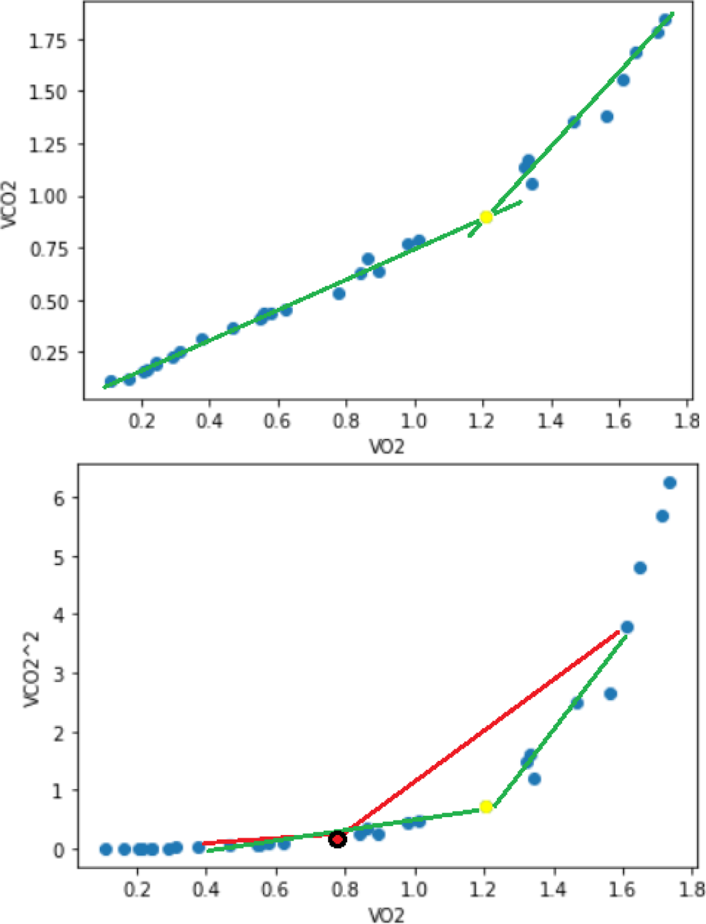
Top: slopes of VO₂ vs VCO₂ plot analysis to detect VT. Bottom: the same variables but with VCO₂ squared, the yellow dot indicates the moment of VT. The yellow dot draws two lines that fit the best with all the dots, while the red dot only fits well with the values behind it.

Expected values for VO₂ peak, and O₂ pulse peak were calculated based on the Study of Health in Pomerania (SHIP) CPET reference equations [17]. Expected values for heart rate at peak exercise were calculated based on reference equations from healthy individuals [18]. We calculated the minimum, maximum, mean, standard deviation, and slope in each quarter of the total time of each CPET. The slope from 15 and 85 percent of all the variables in CPET test time was calculated based on a visual analysis to assess the most stable variable slopes while minimizing noise. In order to isolate the physiological variables from CPET that have the most relevance in the prediction of a patient’s limitation to exercise, the variables age, gender, anthropomorphic measures, and other clinical metrics (e.g., lab values, medical problems, and medications) were ignored. A complete list of the variables used is in the following link (https://dx.doi.org/10.21227/m4h8-z187 ).

C. Feature Selection

After feature engineering, the variables (106 in total) were filtered using the Boruta algorithm, a random forest-based method with the following steps [14, 19]:

• Generate copies of the variables with random data. These copies are shadow attributes; they have no predictive value.

• Shuffle the added variables to eliminate their correlations with the response.

• Create a random forest classifier to evaluate the variables.

• Compute Z scores from the classifier’s variables.

• Find the maximum Z score among shadow attributes (MZSA) and assign a value for each feature that scores better than MZSA.

• For each feature of undetermined importance, perform a two-sided equity test with the MZSA.

• Features with an importance significantly lower than MZSA can be considered unimportant and removed from the system.

• Attributes significantly greater than MZSA are important and remain.

• Remove all shadow attributes.

• Repeat the process until the importance is assigned to all the features or the algorithm reaches its defined limits.

• The iteration assures the selected attributes are not limited to one run.

The Boruta algorithm was applied to each organ system limitation (cardiac, pulmonary, or other system) to identify the most useful features. After the algorithm was run, the features were divided into three groups: important, tentative, and rejected. The “important” group has a strong influence in the model and removing one of the features may reduce the model’s precision. The “tentative” group has some importance, but the contribution is not as strong. The “rejected” group does not provide any improvement to the model. By analyzing the z-scores, the Boruta algorithm chose all the important features with some tentative features for its final selection. It is important to note that the Boruta algorithm’s feature importance may be different from the best performing model. The feature’s order from Boruta is from an iteration of many random forests. The final model is only one algorithm depending on different configuration parameters; this makes its final selection slightly different from Boruta’s algorithm.

D. Classifier

Once the features were selected, automatic machine learning (AutoML) experiments were run in Microsoft Azure Machine Learning to generate different algorithms for primary pulmonary, cardiac, and other system limitations detection. With AutoML the data normalization, model selection, and hyper parameters’ optimization was done automatically. Then, the best performing models with their configurations from the AutoML experiments were chosen. Different experiments on each limitation were run with over 1000 models, including algorithms such as logistic regression, support vector machine, and K-nearest neighbors. Because it had the best results most of the time on each limitation, random forest was selected from all the types of models. This model is a combination of unpruned classification trees created from bootstrapping samples and random feature selection. Random forest predicts by aggregating the prediction from the ensemble of trees [20]. The final models from AutoML were manually tuned using K-fold validation. Due to the size of the data there were five folds, each fold with a similar number of positive cases. The final model was created using 80% of the samples for training.

E. Model Explanation

Given that the output of the random forest models does not produce easy interpretation of the variables that differentially contribute to predictions, we used Shapley Additive Explanations (SHAP) to aid model interpretation. SHAP is a method from coalitional game theory, calculating Shapley values to explain a feature’s contribution [21, 22]. Shapley values do not provide the direct odds of a result, but rather the relative magnitude and direction—either positive or negative—of feature contribution. The combination of all the interpretations in the training dataset creates useful interpretation graphs (i.e., the SHAP summary plot) showing the importance of a feature and the direction of the importance (whether positive, negative, or non-linear). We also used dependency plots generated by plotting all the SHAP values on the y-axis and all the features values on the x-axis [23]; this plot provides the evolution of the Shapley values based on a feature value in the model, giving useful interpretation patterns

F. Dashboard

To visualize information from the classifiers for each case, a custom dashboard was created with the model’s predictions on the patient’s limitations displayed. Once the classifiers and scalers were selected, they were applied to the existing dataset. The patient’s number, description, predictions, and actual label were merged into a table. The dashboard was created with the models, adapters, previous results, and interpretation. The front end was hosted in Amazon Web Service (AWS) and the back end in Azure.

III. RESULTS

A. Data Analysis Summary

From the original 225 CPET cases, 219 cases remained after data processing and the removal of patients with no HR data. From the filtered list, the most common label for primary limitation to exercise was normal (43%), followed by cardiac (24%), other (21%), and pulmonary (12%) (Table I) (Supplemental Table I). The normal group had greater values in several key indicators, most notably for percentage predicted VO₂ peak where the mean for limited individuals was less than 65% versus over 100% for normal. Other observations from this group are the low percentage of females across categories and the similar VO₂ peak (mean and percentage of predicted) between limitation groups.

TABLE I.

PATIENT INFORMATION

	Primary limitation to exercise
Variable	Cardiac	Pulmonary	Other	Normal
Number of cases (%)	51 (24%)	26 (12%)	45 (21%)	95 (43%)
Age: mean (SD)	59.57 (15.48)	51.58 (14.15)	56.33 (15.31)	52.16 (14.66)
Gender: female (%)	14 (7%)	3 (1%)	14 (6%)	44 (20%)
VO2 peak: mean, L/min (SD)	1.42 (0.45)	1.37 (0.61)	1.25 (0.64)	2.45 (0.97)
VO2 peak: % predicted (SD)	63 (15)	60 (25)	57 (15)	107 (28)
Percent VO2 peak at VT: (SD)	35 (12)	32 (16)	34 (11)	57 (21)
HR peak: mean (SD)	136 (28)	145 (20)	132 (28)	168 (21)
O2 pulse at peak: mean, mL/beat (SD)	11.15 (3.7)	9.71 (3.65)	10.33 (3.8)	16.79 (12.23)
VE peak: mean, L/min (SD)	60.13 (15.78)	67.8 (28.77)	53.67 (30.63)	91.74 (34.55)
RER peak: mean (SD)	1.37 (0.25)	1.27 (0.22)	1.18 (0.22)	1.30 (0.21)
VE/VCO2 min: mean (SD)	30.42 (5.26)	35.77 (9.84)	34.81 (7.08)	26.39 (4.27)

B. Cardiac Limitation Model

The Boruta algorithm-selected features were normalized and the model generated based on the AutoML recommendations. For the model’s interpretation, a SHAP summary plot was created where the general model behavior on each feature was described (Figure. 3, top). The complete summary plot for each limitation model can be found in the Supplemental Figure 1. The detailed dependency of the most important feature in the final model is shown in the dependency plot (Figure 3, bottom). Given that the model has 24 features, details of the five most important dependencies are shown in Supplemental Figure 2; the final model had some minor adjustments (see Supplemental Table II for details of each model). The performance from the K-fold validation and the best model are shown in Table II.

Figure 3.

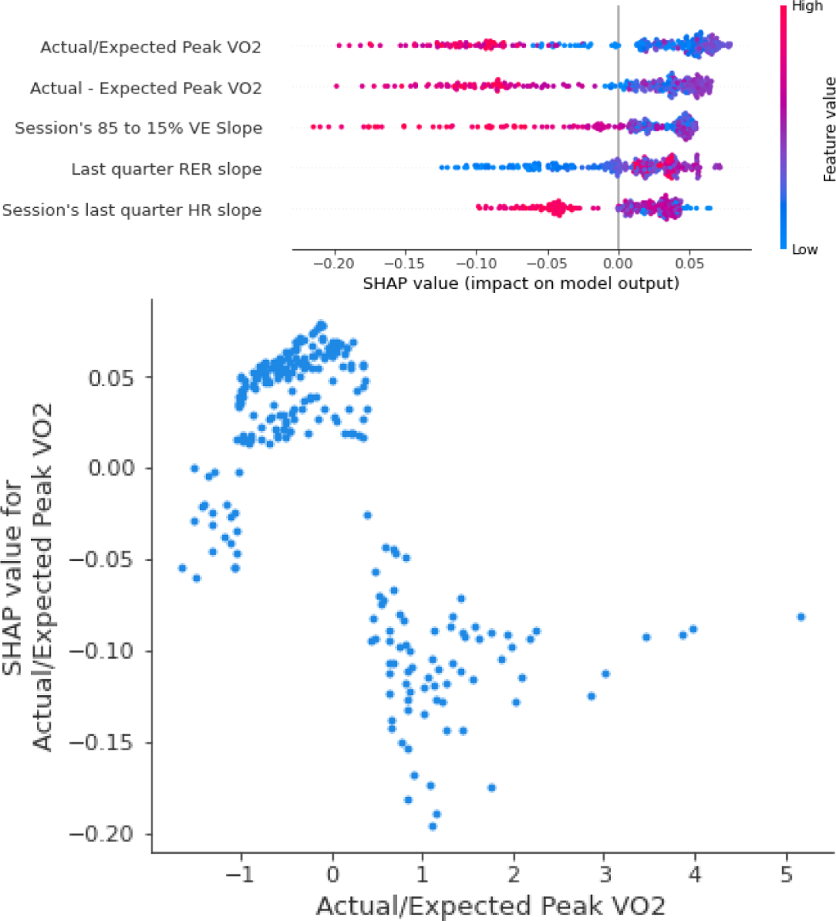
Top: SHAP summary plot for the five most important features in the cardiac limitation model. Positive SHAP values refer to increased odds of having a cardiac limitation, while negative SHAP values refer to decreased odds. The dot color corresponds to the feature’s actual value. For example, for the difference from predicted VO₂ (Actual/Expected Peak VO₂), lower values refer to higher odds of a cardiac limitation. Bottom: the dependency plot for the most important feature in the model showing more details with an inverse relationship between Actual/Expected Peak VO₂ and the SHAP values.

TABLE II.

PERMORMANCE METRICS FOR THE CARDIAC LIMITATION MODEL

	Mean	Std	Best
AUC	0.898	0.062	0.961
Sensitivity	0.762	0.083	0.909
Specificity	0.897	0.031	0.941
Positive Predictive Value	0.696	0.083	0.833
Accuracy	0.866	0.041	0.933

C. Pulmonary Limitation Model

Using the Boruta’s selected features, the final model was chosen from the AutoML specifications and manually tuned to achieve the best generalization possible. As expected, given the small number of cases, its performance metrics were less than the cardiac model. However, its best performing model had good results with a positive predictive value 0.4 (Table III). Compared to the cardiac model, O₂ pulse became more relevant for the model as it was included in three of the eleven predictive variables (Figure 4, Supplemental Figure 1, and Supplemental Figure 3).

TABLE III.

PEFORMANCE METRICS FOR PULMONARYLIMITATION MODEL

	Mean	Std	Best
AUC	0.834	0.066	0.926
Sensitivity	0.5	0.2	0.8
Specificity	0.838	0.024	0.868
Positive Predictive Value	0.285	0.079	0.4
Accuracy	0.798	0.027	0.837

Figure 4.

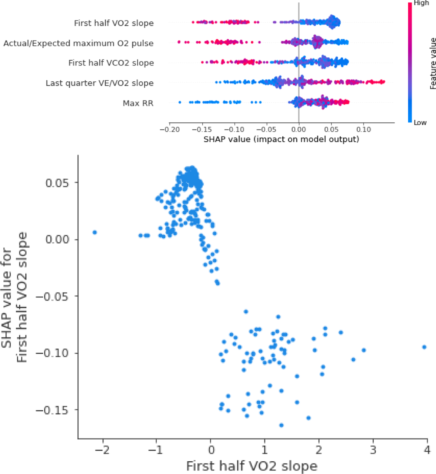
Top: the SHAP summary plot for the five most important features in the pulmonary limitation model. Bottom: the dependency plot for the most important feature in the model.

D. Other Limitations Models

Following the same procedure, the Boruta’s selected features were scaled based on the recommendations. For this limitation, a normalizer was used to scale the data and a random forest with 75 estimators was used for the final model. Its performance metrics, mean and best are in Table IV Also, the configuration, specifications and other details can be seen in the Supplementary Table II. Compared to the other limitation models, this model has 23 variables but only eight with high relevance (Figure 5, Supplemental Figure 1, and Supplemental Figure 4).

TABLE IV.

PERFORMANCE METRICS FOR THE OTHER LIMITATIONS MODEL

	Mean	Std	Best
AUC	0.843	0.110	0.935
Sensitivity	0.600	0.206	0.889
Specificity	0.868	0.082	0.971
Positive Predictive Value	0.575	0.180	0.833
Accuracy	0.812	0.072	0.884

Figure 5.

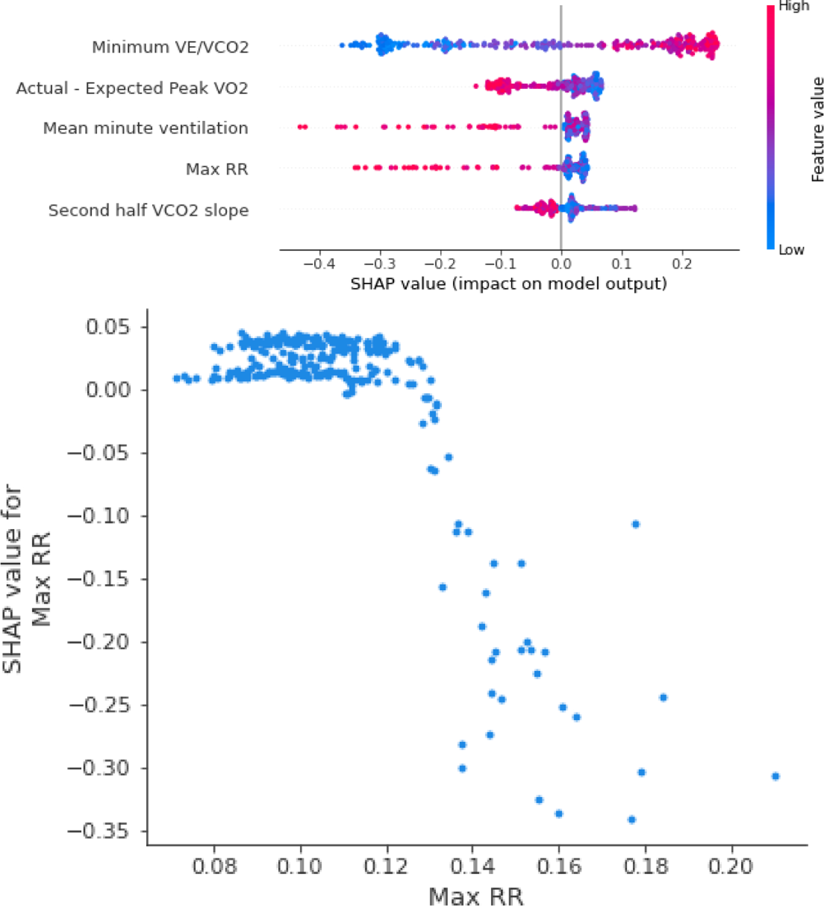
Top: SHAP summary plot for the top five most important features in the other primary limitation model. Bottom: the dependency plot for the most important feature in the model.

E. Dashboard

The dashboard contains three main components. First, the radar plot shows the likelihood of a patient’s primary limitations based on the current dataset (Figure 6). The second component shows the model’s performance at different stages of the CPET session. The last component contains a form where clinicians can upload their own data to achieve results. A model of the full three-component dashboard is shown at http://cpet-radar-plot-duke.s3-website-us-east-1.amazonaws.com/

Figure 6.

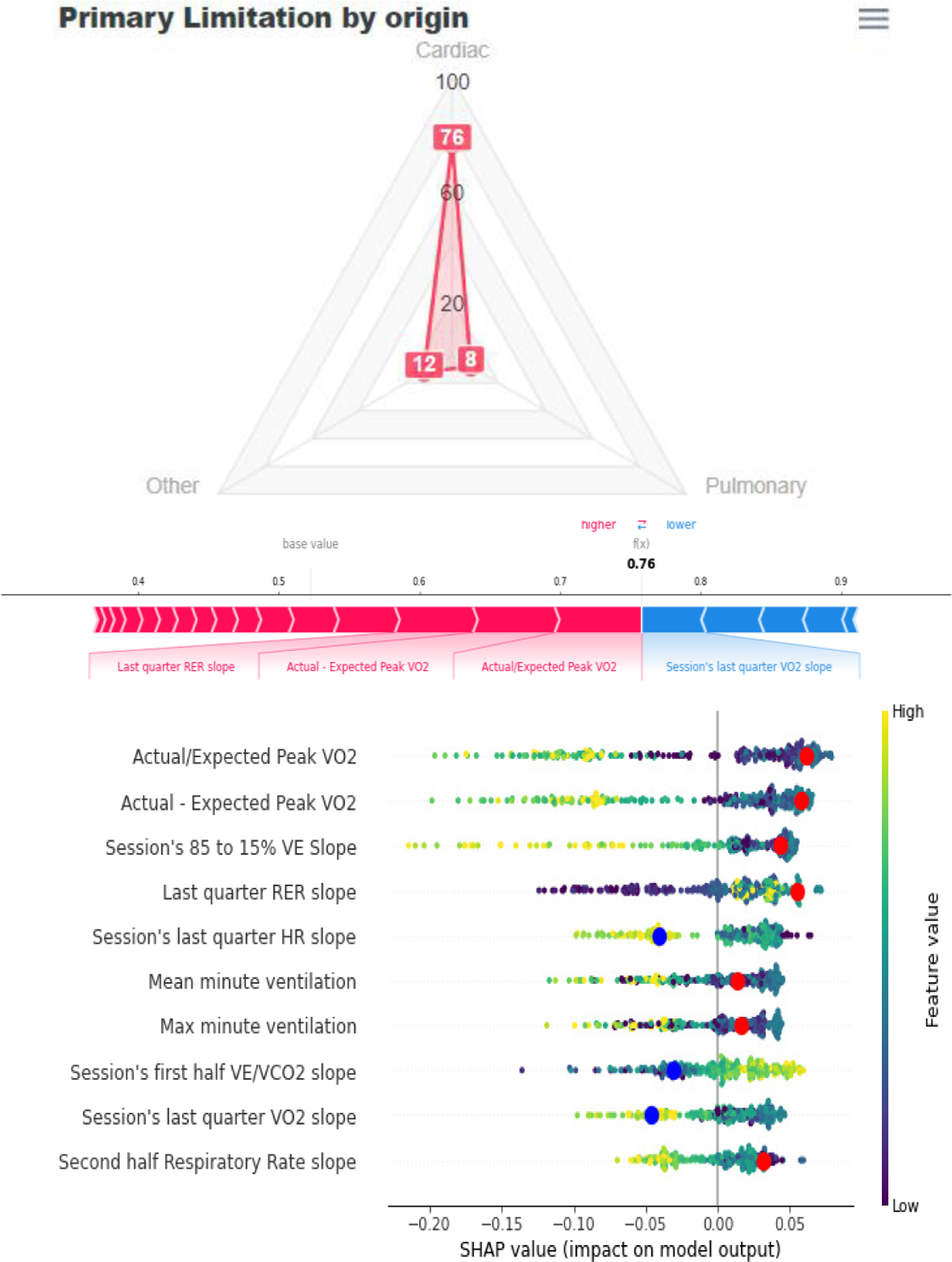
CPET dashboard display. Top: radar plot depicting the model’s predictions. Bottom: explanations for each model shown in a pop-up SHAP force plot (middle) and modified SHAP summary plot function that indicates the patient’s values (red dots for increasing the odds and blue dots for reducing the odds).

To ensure interpretability, the radar plot has three buttons that show two types of complementary SHAP summary plots (Figure 6, Top). A customized SHAP summary plot highlights the features that the model considers in its final decision (See Figure 6, bottom). A force plot then shows the most important features for a particular session (Figure 6, Bottom).

IV. Discussion

A. Clinical Implications

CPET is a valuable, yet underutilized tool for clinician assessment of exercise limitation [23–25]. CPET use is generally confined to the few expert clinicians (i.e., specialized cardiologists, pulmonologists, and exercise physiologists) with the dedicated training and experience needed for interpretation of the considerable data obtained from each test; thus, new ways of analyzing and visualizing CPET data are needed [9, 24, 26]. As a major step forward in CPET data analysis, our platform combines machine learning with a novel interpretive and visualization dashboard to differentiate multiple possible etiologies of exercise limitation (i.e., cardiac, pulmonary, or peripheral/skeletal muscle localizations). For inexperienced users and general clinicians, this machine learning-generated classification system and visualization of the primary exercise limitation (e.g., primary cardiac limitation) guides next steps in diagnosis and clinician-patient communication. For the expert exercise physiologist, the model explanations with SHAP and dependency plots enrich current pathways of CPET interpretation by highlighting specific features relevant to individual patients, aiding in communication about the results with the clinician ordering the test. With further refinement and the addition of more prospective use cases, this machine learning platform can inform clinical care in challenging cases (e.g., the patient with multiple medical co-morbidities with worsening exertional dyspnea or the elite athlete with a new decline in performance). Still, even in its current form, our reported models provide many useful clinical insights to aid CPET data interpretation.

Regarding the cardiac limitation model, the random forest model algorithm identified several patterns predicted by clinical experts. For example, the final cardiac limitation model considers the difference between the maximum expected VO₂ and the actual VO₂ peak (i.e., actual/expected peak VO₂) as the variable with highest predictive power, which is similar to previous clinical findings [8]. Importantly, actual/expected peak VO₂ detected via CPET can help identify patients with heart failure and exercise limitations [8, 27]. Further, in the cardiac limitation model, the slope of the HR response to peak exercise and the related O₂ pulse variables are important predictive features. The comparison between predicted and actual O₂ pulse is useful for detecting cardiac impairment [9]. Finally, the first half of the VE/VCO₂ was considered by the selection algorithm; a high VE/VCO₂ slope has a strong relationship with impaired cardiac outputs and exercise limitation [10, 28, 29]. Interestingly, the lowest VE/VCO₂ value (which is used to predict outcomes in the patients with heart failure using CPET [10]) was not considered by the selection algorithm.

The pulmonary limitation model also selected and sorted features by importance as expected based on current literature regarding CPET; several of these features were similar to the cardiac limitation model. As an example, the difference between the actual and expected VO₂ peak was considered in both cardiac and pulmonary limitation models. VO₂ peak assessment is of also of importance in the detection of patients with obstructive lung diseases [27]. Further, as in the cardiac limitation model, VE/VCO₂ slope was considered in the pulmonary limitation model; an abnormal VE/VCO₂ slope can also be used to detect pulmonary limitations [9, 24], which matches the model’s final selection and feature importance. Finally, the O₂ pulse was considered in both cardiac and pulmonary limitation models; flattening of the O₂ pulse is also associated with reduced body mass and pulmonary hyperinflation [30].

A few key features differentiated cardiac and pulmonary limitation models with potentially important clinical implications. Only the cardiac limitation model considered VO₂ at VT and the slope of HR and RER at the end of the test in its prediction. On the other hand, only the pulmonary limitation model considered RR at peak exercise and the slope of VE/VO₂. Thus, identification of these key by physiological variables may aid in simplified CPET data interpretation by the clinician. For example, a clinician could readily identify a patient as more likely having a cardiac limitation to exercise via CPET measure of a low VO₂ at ventilatory threshold, high HR slope, and normal RR and slope of VE/VO₂ at peak exercise.

Compared to the cardiac and pulmonary limitation models, the other limitations model offered similar—yet more inconsistent—clinical insights. The variable in the other limitations model with the highest predictive value was the minimum VE/VCO₂. This finding of the importance of VE/VCO₂ is not unexpected given that nearly half of the cases used in the other limitations model were from patients with pulmonary hypertension; abnormalities of VE/VCO₂ are common in pulmonary hypertension patients and help distinguish the disease from other causes [26]. One unexpected finding in the other limitations model was that VT derived variables were not selected considering that many of the CPET cases used in the model were patients with primary musculoskeletal system abnormalities. For limitations caused by alterations in skeletal muscle metabolism, VT becomes an important factor as a patient will reach VT early during the test [9]. One possible reason VT was not selected in the model is because of the heterogeneity in clinical cases used, which may have biased the results (See Supplementary Table I).

B. Models

All the models follow the same feature engineering and feature selection process. The features (e.g., expected peak VO₂ vs actual peak VO₂) were proposed by CPET experts. Then, on each model creation we performed a Boruta feature evaluation. The variables considered important were then added to train the final model on each limitation.

Random forest was chosen for the final model for several reasons. First, it was the method with the best results in the AutoML experiments. Deep learning was also considered as a choice, however it requires more samples than random forest without improving the performance metrics [31]. Another useful attribute of random forest is its robustness and computing power it can deal with missing data and needs less computational power to be used in production[31].

The model with the best performance was the cardiac model. The superiority this model was expected because it included many cases from each of the three data sources. On the other hand, the pulmonary model had the lowest performance because it had the lowest number of cases, with the majority coming from the Wasserman textbook.

There are several useful indicators of model performance, including AUC, accuracy, and positive predictive value. For the AUC interpretation, the Fawcett criterion defines tests as follows: 0.5 to 0.6 is a bad test, 0.6 to 0.75 is a regular test, 0.75 to 0.9 is a good test, 0.9 to 0.97 is a very good test, and over 0.97 to 1 is an excellent test [32]. In terms of AUC, the best cardiac model is in the excellent range, the best pulmonary and other models are in the good range e (See Figure 7).

Figure 7.

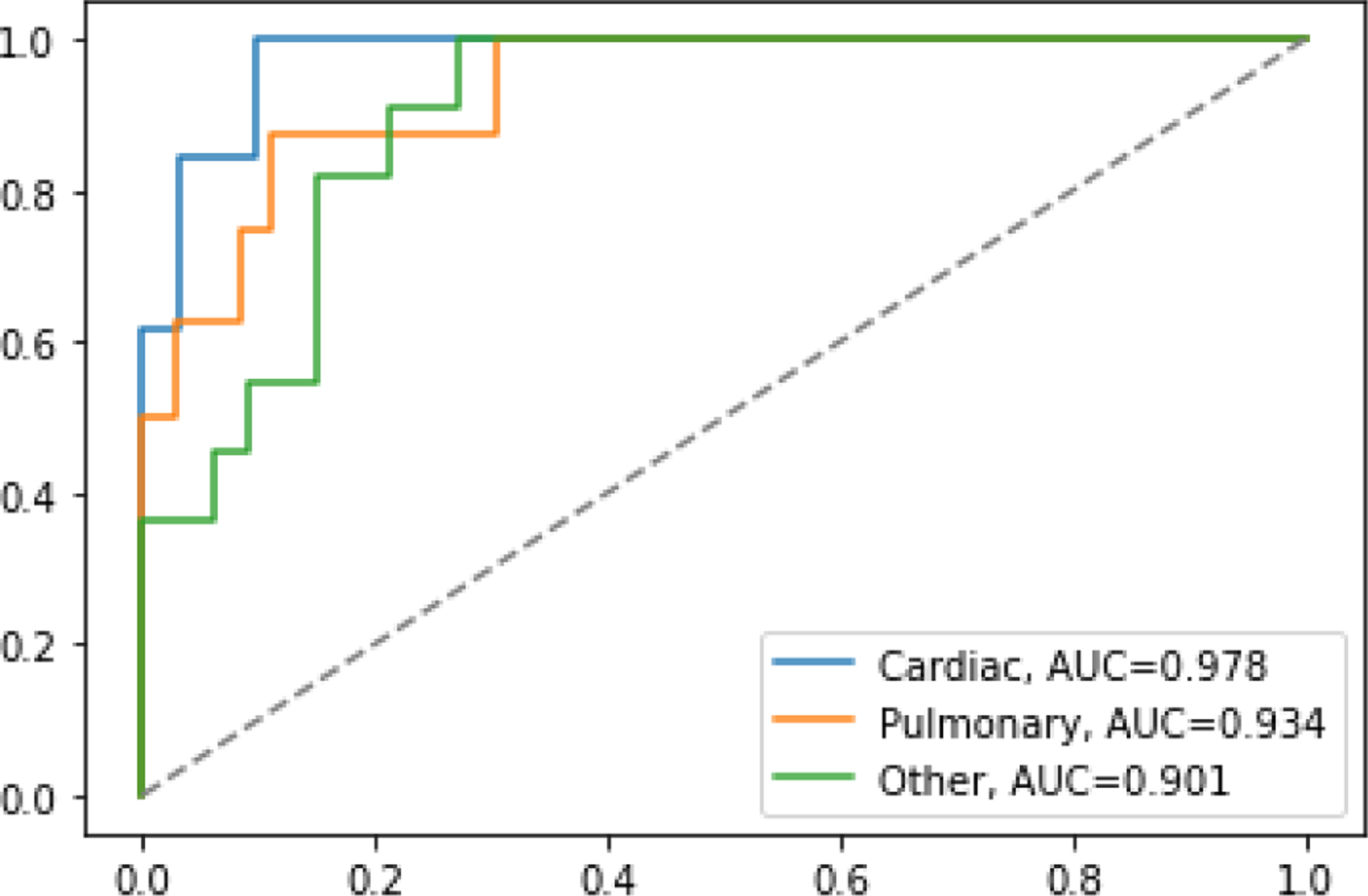
AUC for all the best performing models on the test dataset

C. Technology

We used R for the feature selection and Python for feature engineering, AutoML, and model selection. In the feature engineering and creation phase, the library Pandas was used on a Python Jupyter notebook given its versatility. For feature selection, different libraries were explored in Python and R. For this project we used R with the library Boruta. Compared to the Python equivalent, R’s random Boruta was more effective. AutoML can be used with different tools: AWS Sage Maker autopilot, Vertex AI from Google Cloud Platform (GCP), or Azure Machine Learning Studio. AWS needs at least 500 data samples, and GCP needs at least 1000 data samples. We therefore selected Azure Machine Learning Studio, which has no data size restriction; it also provides a detailed report of the generated models with performance metrics and interpretability.

For the interpretation, the Python SHAP package was used to display the summary and dependency plots. The dashboard evolved from a prototype in R shiny to a website coded in Angular with Material design. This change allowed a cleaner display of the models’ results with the explanation of the scores generated. The dashboard back end was coded in Python using Flask for communication between the service and the front end.

The use of AutoML for the model selection is unique and provided alternatives that are possible with a manual model (e.g., searching for new alternatives and configuration of the data normalization). An advantage of AutoML is that it saves time and energy needed for these tasks [33]. Compared to previous other studies on CPET, the use of SHAP also helps clinicians understand how the algorithm models the features behavior and may be a way to increase adoption of the ML tools.

D. Dashboard

The purpose of the dashboard was to display the information from the machine learning algorithm in a user-friendly way to help clinical decision making. As a means to achieve this goal, the dashboard display provides both simplified outputs from the model and an explanation for its decision. To display the models’ scores, previous CPET data visualization alternatives were used as a baseline [9]. We experimented with display alternatives such as heat maps, reorganization of the plot, and animations, but they were not as simple and user-friendly as the 3D plot alternative. For example, compressing 3D visualizations into two-dimensional images once displayed on a screen or printed can lead to challenges with interpretation; the human eye tries to correct the distortion from 2D back to 3D depending on the angle of the information display [34]. To avoid distortions in display, we used a radar plot as a surrogate 3D plot.

The next step was to provide a graph or a combination of many that will add interpretability to the decision of the ML model. A major challenge in the dashboard was deciding the amount of information to display the plots and how. Although dependency plots provide the most details on how a feature increases or reduces the odds of having a limitation, displaying all or even five of them were not viable to our experts (BJA and WEK), thus, the dependency plots were not considered in the dashboard. Instead, the SHAP summary plot of the 10 most relevant features combined with highlights of the patient’s values (Figure 6, bottom) proved to be clearer. To complement it, a SHAP force plot was used, this shows the most important features in the decision, providing a complementary filter to the clinician for the indicators to look for.

V. LIMITATIONS

The primary limitations of this project are related to the number and type of CPET cases used for analyses. First, only 19 of the 225 CPET cases had primary pulmonary limitations to exercise. As evident by the greater accuracy and predictive power of models with a greater number of cases (i.e., cardiac and other limitations models versus the pulmonary model), the addition of more prospective CPET cases will improve model performance. Further, CPET cases were obtained from a variety of databases, including cases for research and clinical purposes from multiple institutions, in addition to 110 cases transcribed from the “Principles of Exercise Testing and Interpretation” textbook by Wasserman et al.[1]. While cases from the Wasserman textbook provided an additional source of case variety encompassing a large spectrum of disease states, these cases also skewed toward more severe manifestations of disease. Given that a majority of primary pulmonary limitation cases came from the Wasserman textbook, the results of this study need to be interpreted with caution as some of the machine learning features differentiating pulmonary versus cardiac and other limitations may be detecting disease severity as opposed to intrinsic differences in those conditions. Regardless, average peak heart rates and fitness levels from the CPET cases did not significantly differ between groups (see Table I). The addition of prospective data in future work should eliminate potential bias in the current analyses. Finally, the “other” category for defining exercise limitation with CPET was from a heterogeneous group of multiple dissimilar disease states (e.g., pulmonary hypertension, peripheral vascular disease, and muscle metabolic disease). This categorization of exercise limitation was purposely chosen given the small number of CPET cases available, with the primary purpose to differentiate these cases from the most clinically relevant cardiac or pulmonary etiologies.

Compared to previous research using SVM to aid CPET data interpretation, we included a lower number of cases in the dataset [15]; however, their target study outcome was more specific and their datasets more uniform. Further, we used broader definitions to label cases as chronic heart failure and the obstructive pulmonary disease definitions, which may make our data more susceptible to errors.

Regarding the model, using three types of limitations may be broad, especially for the other origin type. Many cardiac and pulmonary causes of exercise limitation have common interpretability patterns that match the experts’ knowledge. However, cases used in the other limitations model include patients with a variety of disease-states. This likely explains why the model chose different variables compared to those recommended by the experts (i.e., VT). Other cases can also be classified as a mix of pulmonary and cardiac which difficult the effectiveness of the classifier and the detection of expected patterns. Given these diverse disease-states and inclusion of few cases, detection and interpretation of the other limitations was more challenging compared to primary cardiac and pulmonary limitations. Finally, inclusion of cases performed using different CPET protocols (i.e., treadmill and cycle ergometer) restricts the number of variables used in our modeling to those universally detected across protocols. For example, estimation of work rate via CPET may improve the performance of the cardiac model [26]; however, work rate can only be reliably assessed using cycle ergometer protocols.

VI. Conclusion

CPET assesses critical components of human health (i.e., exercise capacity and limitations to exercise) that are not commonly considered in clinical practice due to challenges with data interpretation. In this project, we used a machine learning process that creates the features, filters them, and creates models to successfully differentiate patients with cardiac, pulmonary, or other organ-system limitations to exercise. Our platform provides both simplified CPET analysis output to aid general clinician-patient communication and more detailed feature analysis to inform and help the expert exercise physiologist understand individual responses to exercise. More robust and accessible exercise testing data interpretation platforms will aid clinical decision making across a wide spectrum of cardiopulmonary disorders to enhance the care of patients with chronic diseases.

VII. FUTURE DIRECTIONS

In all the cases, the models’ prediction of the primary organ-system limiting exercise incorporated CPET variables similar to expert classification. With the addition of prospective case samples, the patterns detected can be corroborated and uncovered for all the limitations. Furthermore, with additional and more diverse data samples we anticipate that the subtypes of exercise limitations can be detected.

Further additional work includes the use of neural networks to explore if there is a better model and interpretation for identifying limitations to exercise with CPET. An advantage of neural networks is that they analyze non-linearities appearing in time series data usually lost during features engineering. With interpretation algorithms such as Gradient-Weighted Class Activation Mapping, neural networks can show the visual patterns on the signals comparable to a physician’s interpretation. The main disadvantage of neural networks is the large number of training samples needed to be effective.

Another approach for improving model performance is to capture and use earlier CPET data to process into features before the middle of the session. Early data capture would allow for exercise limitation assessment in patients who are unable to complete a maximal CPET session (e.g., pediatric and very elderly patients). By having an accurate diagnostic without the need for maximal or peak CPET data, a patient may not need to complete the entire CPET session to assess their exercise limitations.

Currently our CPET dashboard display is for research purposes. It was developed as a proof-of-concept to show the model’s performance using real clinical cases. Changes to the dashboard will be needed to incorporate into clinical settings (e.g., inputs could be added manually or through software that completes feature engineering automatically). Future dashboard changes will be based on feedback from the users (e.g., clinicians and exercise physiology specialists) regarding the benefits and usability of the models and interpretation graphs.

Nomenclature.

Key terms are defined as follows:

• VO₂ (Oxygen consumption): rate of oxygen consumption expressed in absolute terms (mL/min), (L/min) or relative (mL/kg/min).

• VO₂ peak (Peak oxygen consumption): greatest rate of oxygen consumption during maximal progressive exercise; a measure of cardiorespiratory fitness.

• VCO₂ (Carbon dioxide production): rate of carbon dioxide exhaled (mL/min).

• HR (Heart Rate): number of beats per minute (bpm); a variable progressing from less than 100 bpm while resting and increasing during progressive exercise to a peak.

• VE (Minute ventilation): volume of air exhaled per minute (L/min).

• RER (Respiratory exchange ratio): molar ratio of CO₂ produced per O₂ consumed; a variable progressing from less than 0.80 to greater than 1.10 during progressive exercise.

• RR (Respiratory Rate): number of breaths per minute.

• O₂ pulse (Oxygen pulse): volume of oxygen uptake per heartbeat (VO₂/HR; mL/beat); an alternative measure for stroke volume.

• VE/VCO₂ (Slope of minute ventilation versus carbon dioxide production): measurement of ventilatory efficiency or dead space ventilation.

• VT (Ventilatory threshold): point in time when ventilation disproportionally increases compared to oxygen consumption (VO₂ @ VT (mL/min) or HR at VT (beats/min)); reflects increased energy demands from anaerobic metabolism.

REFERENCES

- [1].Wasserman K, Hansen JE, and Sue DY, “Principles of Exercise Testing and Interpretation : Including Pathophysiology and Clinical Applications,” (in English), 2015. [Online]. Available: http://qut.eblib.com.au/patron/FullRecord.aspx?p=2031851. [Google Scholar]
- [2].Balady GJ et al. , “Clinician’s Guide to cardiopulmonary exercise testing in adults: a scientific statement from the American Heart Association,” Circulation, vol. 122, no. 2, pp. 191–225, Jul 13 2010, doi: 10.1161/CIR.0b013e3181e52e69. [DOI] [PubMed] [Google Scholar]
- [3].Hunt SA et al. , “ACC/AHA 2005 Guideline Update for the Diagnosis and Management of Chronic Heart Failure in the Adult: a report of the American College of Cardiology/American Heart Association Task Force on Practice Guidelines (Writing Committee to Update the 2001 Guidelines for the Evaluation and Management of Heart Failure): developed in collaboration with the American College of Chest Physicians and the International Society for Heart and Lung Transplantation: endorsed by the Heart Rhythm Society,” Circulation, vol. 112, no. 12, pp. e154–235, Sep 20 2005, doi: 10.1161/CIRCULATIONAHA.105.167586. [DOI] [PubMed] [Google Scholar]
- [4].Albouaini K, Egred M, Alahmar A, and Wright DJ, “Cardiopulmonary exercise testing and its application,” Heart, vol. 93, no. 10, pp. 1285–92, Oct 2007, doi: 10.1136/hrt.2007.121558. [DOI] [PMC free article] [PubMed] [Google Scholar]
- [5].Boyd J, Powell P, Vogiatzis I, Kontopidis D, and Hebestreit H, “Cardiopulmonary exercise testing (CPET) patient survey,” European Respiratory Journal, vol. 52, no. suppl 62, p. PA2473, 2018, doi: 10.1183/13993003.congress-2018.PA2473. [DOI] [Google Scholar]
- [6].Maeder MT, “[Cardiopulmonary exercise testing for the evaluation of unexplained dyspnea],” Ther Umsch, vol. 66, no. 9, pp. 665–9, Sep 2009, doi: 10.1024/0040-5930.66.9.665. Stellenwert der Spiroergometrie in der Diagnostik der Belastungsdyspnoe. [DOI] [PubMed] [Google Scholar]
- [7].Hansen JE, Sun XG, and Stringer WW, “A simple new visualization of exercise data discloses pathophysiology and severity of heart failure,” J Am Heart Assoc, vol. 1, no. 3, p. e001883, Jun 2012, doi: 10.1161/JAHA.112.001883. [DOI] [PMC free article] [PubMed] [Google Scholar]
- [8].Dumitrescu D and Rosenkranz S, “Graphical Data Display for Clinical Cardiopulmonary Exercise Testing,” Ann Am Thorac Soc, vol. 14, no. Supplement_1, pp. S12–S21, Jul 2017, doi: 10.1513/AnnalsATS.201612-955FR. [DOI] [PubMed] [Google Scholar]
- [9].Andonian BJ, Hardy N, Bendelac A, Polys N, and Kraus WE, “Making Cardiopulmonary Exercise Testing Interpretable for Clinicians,” Curr Sports Med Rep, vol. 20, no. 10, pp. 545–552, Oct 1 2021, doi: 10.1249/JSR.0000000000000895. [DOI] [PMC free article] [PubMed] [Google Scholar]
- [10].Myers J et al. , “The lowest VE/VCO2 ratio during exercise as a predictor of outcomes in patients with heart failure,” J Card Fail, vol. 15, no. 9, pp. 756–62, Nov 2009, doi: 10.1016/j.cardfail.2009.05.012. [DOI] [PMC free article] [PubMed] [Google Scholar]
- [11].Hearn J et al. , “Neural Networks for Prognostication of Patients With Heart Failure,” Circ Heart Fail, vol. 11, no. 8, p. e005193, Aug 2018, doi: 10.1161/CIRCHEARTFAILURE.118.005193. [DOI] [PubMed] [Google Scholar]
- [12].Zignoli A et al. , “Expert-level classification of ventilatory thresholds from cardiopulmonary exercising test data with recurrent neural networks,” Eur J Sport Sci, vol. 19, no. 9, pp. 1221–1229, Oct 2019, doi: 10.1080/17461391.2019.1587523. [DOI] [PubMed] [Google Scholar]
- [13].Zignoli A et al. , “Oxynet: A collective intelligence that detects ventilatory thresholds in cardiopulmonary exercise tests,” Eur J Sport Sci, pp. 1–11, Jan 31 2021, doi: 10.1080/17461391.2020.1866081. [DOI] [PubMed] [Google Scholar]
- [14].Maeda-Gutierrez V et al. , “Distal Symmetric Polyneuropathy Identification in Type 2 Diabetes Subjects: A Random Forest Approach,” Healthcare (Basel), vol. 9, no. 2, Feb 1 2021, doi: 10.3390/healthcare9020138. [DOI] [PMC free article] [PubMed] [Google Scholar]
- [15].Inbar O, Inbar O, Reuveny R, Segel MJ, Greenspan H, and Scheinowitz M, “A Machine Learning Approach to the Interpretation of Cardiopulmonary Exercise Tests: Development and Validation,” Pulm Med, vol. 2021, p. 5516248, 2021, doi: 10.1155/2021/5516248. [DOI] [PMC free article] [PubMed] [Google Scholar]
- [16].Mezzani A, “Cardiopulmonary Exercise Testing: Basics of Methodology and Measurements,” Ann Am Thorac Soc, vol. 14, no. Supplement_1, pp. S3–S11, Jul 2017, doi: 10.1513/AnnalsATS.201612-997FR. [DOI] [PubMed] [Google Scholar]
- [17].Koch B et al. , “Reference values for cardiopulmonary exercise testing in healthy volunteers: the SHIP study,” Eur Respir J, vol. 33, no. 2, pp. 389–97, Feb 2009, doi: 10.1183/09031936.00074208. [DOI] [PubMed] [Google Scholar]
- [18].Tanaka H, Monahan KD, and Seals DR, “Age-predicted maximal heart rate revisited,” J Am Coll Cardiol, vol. 37, no. 1, pp. 153–6, Jan 2001, doi: 10.1016/s0735-1097(00)01054-8. [DOI] [PubMed] [Google Scholar]
- [19].Kursa MB and Rudnicki WR, “Feature Selection with the Boruta Package,” 2010, vol. 36, no. 11, p. 13, 2010–09-16 2010, doi: 10.18637/jss.v036.i11. [DOI] [Google Scholar]
- [20].Svetnik V, Liaw A, Tong C, Culberson JC, Sheridan RP, and Feuston BP, “Random forest: a classification and regression tool for compound classification and QSAR modeling,” J Chem Inf Comput Sci, vol. 43, no. 6, pp. 1947–58, Nov-Dec 2003, doi: 10.1021/ci034160g. [DOI] [PubMed] [Google Scholar]
- [21].Lundberg SM and Lee S-I, “A unified approach to interpreting model predictions,” presented at the Proceedings of the 31st International Conference on Neural Information Processing Systems, Long Beach, California, USA, 2017. [Google Scholar]
- [22].Štrumbelj E and Kononenko I, “Explaining prediction models and individual predictions with feature contributions,” Knowledge and Information Systems, vol. 41, no. 3, pp. 647–665, 2014/12/01 2014, doi: 10.1007/s10115-013-0679-x. [DOI] [Google Scholar]
- [23].Molnar C, Interpretable machine learning : a guide for making black box models explainable. (in English), 2020. [Google Scholar]
- [24].Guazzi M, Arena R, Halle M, Piepoli MF, Myers J, and Lavie CJ, “2016 Focused Update: Clinical Recommendations for Cardiopulmonary Exercise Testing Data Assessment in Specific Patient Populations,” Circulation, vol. 133, no. 24, pp. e694–711, Jun 14 2016, doi: 10.1161/CIR.0000000000000406. [DOI] [PubMed] [Google Scholar]
- [25].Irvin CG and Kaminsky DA, “Exercise for fun and profit: joint statement on exercise by the American Thoracic Society and the American College of Chest Physicians,” Chest, vol. 125, no. 1, pp. 1–3, Jan 2004, doi: 10.1378/chest.125.1.1. [DOI] [PubMed] [Google Scholar]
- [26].Guazzi M et al. , “EACPR/AHA Scientific Statement. Clinical recommendations for cardiopulmonary exercise testing data assessment in specific patient populations,” Circulation, vol. 126, no. 18, pp. 2261–74, Oct 30 2012, doi: 10.1161/CIR.0b013e31826fb946. [DOI] [PMC free article] [PubMed] [Google Scholar]
- [27].Guazzi M, “How to interpret cardiopulmonary exercise tests,” Heart and Metabolism, Article no. 64, pp. 31–36, 2014. [Online]. Available: http://www.scopus.com/inward/record.url?scp=84908475851&partnerID=8YFLogxK. [Google Scholar]
- [28].Arena R, Myers J, Aslam SS, Varughese EB, and Peberdy MA, “Prognostic Comparison of the Minute Ventilation/Carbon Dioxide Production Ratio and Slope in Patients with Heart Failure,” Heart Drug, vol. 4, no. 3, pp. 133–139, 2004, doi: 10.1159/000078907. [DOI] [Google Scholar]
- [29].Mejhert M, Linder-Klingsell E, Edner M, Kahan T, and Persson H, “Ventilatory variables are strong prognostic markers in elderly patients with heart failure,” Heart, vol. 88, no. 3, pp. 239–43, Sep 2002, doi: 10.1136/heart.88.3.239. [DOI] [PMC free article] [PubMed] [Google Scholar]
- [30].Chuang ML, Lin IF, Huang SF, and Hsieh MJ, “Patterns of Oxygen Pulse Curve in Response to Incremental Exercise in Patients with Chronic Obstructive Pulmonary Disease - An Observational Study,” Sci Rep, vol. 7, no. 1, p. 10929, Sep 7 2017, doi: 10.1038/s41598-017-11189-x. [DOI] [PMC free article] [PubMed] [Google Scholar]
- [31].Roßbach P, “Neural Networks vs. Random Forests–Does it always have to be Deep Learning,” Germany: Frankfurt School of Finance and Management, 2018. [Google Scholar]
- [32].Fawcett T, “An introduction to ROC analysis,” Pattern Recognition Letters, vol. 27, no. 8, pp. 861–874, 2006/06/01/2006, doi: 10.1016/j.patrec.2005.10.010. [DOI] [Google Scholar]
- [33].Kulkarni GN, Ambesange S, Vijayalaxmi A, and Sahoo A, “Comparision of diabetic prediction AutoML model with customized model,” in 2021. International Conference on Artificial Intelligence and Smart Systems (ICAIS), 25–27 March 2021 2021, pp. 842–847, doi: 10.1109/ICAIS50930.2021.9395775. [DOI] [Google Scholar]
- [34].Wilke C, “Fundamentals of data visualization : a primer on making informative and compelling figures,” (in English), 2019. [Online]. Available: https://search.ebscohost.com/login.aspx?direct=true&scope=site&db=nlebk&db=nlabk&AN=2087271. [Google Scholar]
Associated Data
This section collects any data citations, data availability statements, or supplementary materials included in this article.