Abstract
This paper studies how people make decisions over preventive behaviors under ambiguity (i.e., Knightian uncertainty) where they do not even know the probability of a loss. In the context of the current COVID-19 pandemic, scientific uncertainty makes it hard to evaluate not only whether one will be infected, but also probabilities such as the infection rate. We constructed a simple model and demonstrated how its effect was heterogeneous depending on ambiguity-attitudes. Motivated by the model, we further conducted a survey experiment in Japan where we manipulated the information regarding scientific uncertainty on COVID-19. We found that higher ambiguity induced by scientific uncertainty increased the level of social distancing among ambiguity-loving people, but such evidence was nonexistent for ambiguity-averse counterparts.
Supplementary Information
The online version contains supplementary material available at 10.1007/s42973-022-00120-3.
Keywords: Scientific uncertainty, Ambiguity, Self-protection, Preventive behaviors, COVID-19
Introduction
In our daily lives, people engage in all kinds of preventive activities to avert losses. For example, a driver’s high attention level decreases the probability of a car accident, and a patient’s health investment makes him or her less likely to be sick. Although such self-protection has been extensively analyzed (e.g., Chiu, 2000; Eeckhoudt & Gollier, 2005; Peter, 2017), the bulk of this literature assumes that people know the probability of a loss, which, however, is not always readily available given the complexity of the real world. As a matter of fact, people oftentimes face ambiguity (i.e., Knightian uncertainty), where such a probability is elusive. As Ellsberg (1961) shows in his famous experiment, people’s decision-making under ambiguity is different from that under risk where its probability is known. Motivated by this fact, several existing studies have theoretically analyzed the self-protection under ambiguity (Alary et al., 2013; Snow, 2011). However, its empirical literature is still quite scarce and underdeveloped. This study therefore aims at filling this gap by leveraging the recent outbreak of COVID-19 (the novel coronavirus disease) in Japan.
While scientists worldwide have been devoting tremendous efforts to understanding the nature of COVID-19, in an early stage of this global pandemic, it was hard to answer questions regarding the nature of the virus, the transmission, or its mutations. For example, the percentage of people who are infected with the novel coronavirus yet asymptotic can be uncertain. Back in April 2020, Dr. Anthony Fauci, the then head of the US National Institute of Allergy and Infectious Diseases, used to say,
“It’s somewhere between 25 and 50 percent. [...] I don’t have any scientific data yet. You know when we’ll get the scientific data? When we get those antibody tests out there.”1
Apparently, lacking enough data for investigating the nature of such an emerging infectious disease, even scientists do not fully understand it. The resulting scientific uncertainty therefore makes it even harder for non-experts to evaluate COVID-19’s rates of infection and mortality in probabilistic terms and forces them to face ambiguity when determining the level of preventive behavior such as social distancing they should adopt. The informational environment of COVID-19 therefore provides an exceptional opportunity and realistic setting for conducting an empirical analysis of the effect of ambiguity on preventive behavior.
To identify the causal effect of ambiguity caused by scientific uncertainty, we first developed a theoretical model. Next, given the ethical concerns over manipulating ambiguity and measuring its effect on people’s real-life preventative behvaiors amid the pandemic, we joined the recent burgeoning literature of online information experiments (Alesina et al., 2018; Kuziemko et al., 2014, 2015; Karadja et al., 2017; Weinzierl, 2018). Specifically, we conducted a survey experiment where each subject was randomly assigned the information about scientific uncertainty and asked to state his or her beliefs and preferences over social distancing.
On the theoretical front, we introduced ambiguity into a standard model of self-protection by using -Maxmin expected utility (-MEU) theory, which was first suggested by Hurwicz (1951) and has been adopted by various applied studies. The advantage of -MEU is that it allows us to separate the degree of ambiguity from ambiguity-attitudes and to deal with ambiguity-loving as well as ambiguity-aversion. By utilizing these two distinctive features of -MEU, we prove that the effect of higher ambiguity depends on situations. In one scenario, higher ambiguity encourages preventive behavior only among ambiguity-loving people, whereas in the other scenario, it does so only among ambiguity-averse ones. That is, the effect of higher ambiguity is expected to be heterogeneous depending on ambiguity-attitudes. Furthermore, the direction of the effect cannot be uniquely determined in theory for the COVID-19 case, and thus empirical analysis is essential.
Our empirical analysis was motivated by this theoretical framework and we conducted an online survey experiment on approximately 1600 individuals in Japan in early July, 2020.2 In Japan, the government’s preventative measures were not legally binding even under the declared state of emergency, and therefore had to depend on citizens’ cooperation to be effective. We took advantage of this special Japanese context to analyze the effect on one’s voluntary decision of social distancing. In the experiment, each respondent was randomly assigned to either the treatment group where the scientific uncertainty about COVID-19 was presented, or the control group where such uncertainty was removed. After this step, we asked if they would go outside in various hypothetical situations during the outbreak of COVID-19. The same information treatment can predict different effects depending on whether subjects are ambiguity-averse or ambiguity-loving. As a result, even an effective intervention may produce average treatment effects that spuriously appear to be null results. To deal with this issue, we measured each respondent’s degree of ambiguity-attitude by using Ellsberg (1961)’s two urn experiments.
The results are summarized as follows. First, as expected, the average treatment effect on one’s social distancing decision is found to be statistically insignificant. Since the effect could be heterogeneous depending on one’s attitude toward ambiguity, we then explored causal heterogeneities by splitting our data into three sub-samples: ambiguity-averse, ambiguity-loving, and ambiguity-neutral respondents. We found that the treatment information substantially increased the level of social distancing among those who were ambiguity-loving, whereas such effect did not exist among either ambiguity-averse or ambiguity-neutral subjects. This result is robust across four different scenarios along two important dimensions in the transmission of the novel coronavirus: (1) crowdedness of a location (high versus low) and (2) mask-wearing (yes versus no). That is, higher uncertainty induces social distancing only among ambiguity-loving respondents. When communicating scientific uncertainty to the public, governments and experts should take this heterogeneous effect on preventive behavior into account.
Related literature: From a theoretical side, several existing studies analyze self-protection under ambiguity. Specifically, based on the smooth ambiguity model à la Klibanoff et al. (2005), Snow (2011) and Alary et al. (2013) show that whether more ambiguity-aversion reduces preventive behavior is contingent on situations.3 Our model has two distinctive features. First, instead of the degree of ambiguity, they actually derive their comparative statics with respect to the degree of ambiguity-attitudes. Second, their model does not allow agents to be ambiguity-loving.
From an empirical side, the effects of scientific uncertainty on both beliefs and behavior have been extensively studied in the literature of risk communication for topics such as risk perceptions in food—as well as health-related fields (e.g., Johnson & Slovic, 1995; Miles & Frewer, 2003) and trust toward scientists (e.g., Teitelbaum, 2007).
Compared to our study, Han et al. (2018) conducted in Spain a similar survey experiment where subjects read one of three versions of a hypothetical newspaper article describing a vaccine-preventable pandemic, but varying in scientific uncertainty. They found that uncertainty reduced vaccination intentions and argued that this was induced by ambiguity-aversion. Our study has three distinctive features vis-á-vis theirs. First, their study was about a hypothetical infectious disease, while ours featured the information of scientific uncertainty regarding a real and ongoing pandemic. Second, the type of preventive behavior is different. In the case of vaccination, the risk of preventive behavior is uncertain, whereas such uncertainty is absent in social distancing. Third, they did not measure ambiguity-attitudes in a rigorous manner, whereas we did it based on Ellsberg’s two-urn experiments and investigated how the effect of scientific uncertainty was interacted with ambiguity-attitudes.
Moreover, another closely related study is Kreps and Kriner (2020), where the authors show experimentally that scientific uncertainty regarding COVID-19 could lead to a distrust in both science and science-based policies. Compared to them, our study has a richer setting where we incorporated two measures of scientific uncertainty and different individual attitudes towards ambiguity.4
The remainder of the paper is organized as follows. Section 2 presents theoretical hypotheses. Sections 3 and 4 explain our experimental design, and Sect. 5 presents empirical results. Section 6 concludes.
Theoretical framework
Setting
To fix the idea, let us consider a single-person decision-making problem where an individual chooses a level of preventive behaviors: . The individual faces uncertainty about whether she or he will be infected. The state space is given by , where I represents infection, and S represents no infection. The infection rate is determined depending on the value of e,5 and thus the expected utility given e is
where V(I) is the material payoff when she or he is infected, V(S) is the payoff when she or he is not, and C(e) is the cost of preventive behaviors. Note that , , and are assumed. So far, the model is the standard model of self-protection, which has been widely analyzed in the literature, although we interpret the model in terms of COVID-19.
In standard models, it is assumed that (the probability of infection) is known to citizens. However, for emerging infectious diseases such as COVID-19, this is not the case due to scientific uncertainty. In other words, scientific uncertainty inevitably creates ambiguity (i.e., Knightian uncertainty), where people do not even know the probability distribution, . Motivated by this fact, we adopt the -Maxmin expected utility theory, which was first suggested by Han et al. (2018) and has been adopted by various applied studies. That is, an individual has a set of candidates for the true probability: . Having this in mind, she or he maximizes the weighted average of the maximum expected utility and the minimum expected utility:
Because the true probability is uncertain, an individual takes both the worst and the best cases into account. The decision weight for the best case is represented by . Hence, can be interpreted as the degree of ambiguity-loving. On the contrary, how large is represents the degree of ambiguity.
To specify , we suppose that is parameterized by a positive real number k: , where Higher k implies the higher marginal effectiveness of preventive behaviors. We describe ambiguity by introducing uncertainty about the value of k.6 That is,
In this specification, higher leads to an expansion of , and thus it represents higher ambiguity. Note that , and are assumed. The effect of higher ambiguity on the optimal level of preventive behaviors, , is different depending on whether b(k, e) is increasing in k.7
Theoretical result
The effect of higher ambiguity on is derived as follows:
Proposition 1
-
(i)
Let b(k, e) be decreasing in k. On the one hand, when is sufficiently high, is decreasing in . On the other hand, when is sufficiently low, is increasing in .8
-
(ii)
Let b(k, e) be increasing in k. On the one hand, when is sufficiently high, is increasing in . On the other hand, when is sufficiently low, is decreasing in .
To see the intuitive mechanism, suppose first that the marginal effectiveness of preventive behaviors and the probability of a loss (i.e., k and ) are positively correlated. This is the case (i) in the above proposition.9 In this case, the agent’s utility is rewritten as
Hence, when , higher implies the lower perceived marginal effectiveness, discouraging preventive behaviors. On the contrary, when , higher implies the higher perceived marginal effectiveness, inducing preventive behaviors. Since similar properties hold as long as is close to one or zero, it is shown that higher ambiguity induces preventive behaviors only among ambiguity-averse agents.
To put it differently, the ambiguity-averse (resp. ambiguity-loving) agents are pessimistic (resp. optimistic) so that they expect that the probability of a loss is higher (resp. lower) in the presence of higher ambiguity. Since this implies the higher (resp. lower) marginal effectiveness of preventive behaviors for the ambiguity-averse (resp. ambiguity-loving) agents, higher ambiguity induces preventive behaviors only among ambiguity-averse agents.
On the other hand, the opposite can be the case in a different situation. To see this, next suppose that the marginal effectiveness of preventive behaviors and the probability of a loss are negatively correlated, which is the case (ii) in the above proposition.10 In this situation, the agent’s utility is rewritten as
That is, the ambiguity-averse (resp. ambiguity-loving) agents, who are pessimistic (resp. optimistic), expect that the marginal effectiveness of preventive behaviors is smaller (resp. larger) in the presence of higher ambiguity. Hence, higher ambiguity induces preventive behaviors only among ambiguity-loving agents.
Hypotheses in the context of COVID-19 outbreak
In the context of social distancing under the COVID-19 outbreak, both cases in the above proposition can be plausible. On the one hand, for example, a determinant of the marginal effectiveness of social distancing is the expected number of infected people one would contact with when going outside. Suppose that k represents this expected number of infected people. Since the probability of infection is obviously increasing in this value, the positive correlation between k and is expected. That is, the situation can be regarded as case (i) in the proposition. If the ambiguity is stemming from uncertainty about this factor, higher ambiguity induces social distancing among ambiguity-averse people.
On the other hand, another determinant of the marginal effectiveness of social distancing is whether their family members are infected. One’s social distancing reduces the probability of infection only when his or her family members living in the same place are unlikely to be infected. Otherwise, he or she will be infected anyway. Hence, the marginal effectiveness of social distancing is increasing in the likelihood of the family members not being infected. Suppose that k represents the probability of one’s family members not being infected. Since the probability of one’s infection is obviously decreasing in this value, the negative correlation between k and is expected. That is, the situation can be regarded as case (ii) in the proposition. If the ambiguity is stemming from uncertainty about this factor, higher ambiguity rather induces social distancing among ambiguity-loving people.
Consequently, we have the following two competing hypotheses:
Hypothesis 1: Higher ambiguity encourages (resp. reduces) social distancing among ambiguity-averse (resp. ambiguity-loving) agents.
Hypothesis 2: Higher ambiguity encourages (resp. reduces) social distancing only among ambiguity-loving (resp. ambiguity-averse) agents.
Since the direction of its effect cannot be uniquely determined in theory and both scenarios can be plausible, empirical analysis is essential. Motivated by this theoretical framework, we next turn to our empirical analysis in the particular context of COVID-19.
The survey
Data collection and sample
In total, 1581 adults in Japan were recruited11 from the online panel (with a size of 2.2 million Japanese members (Rakuten Insight, 2020)) maintained by the Rakuten Insight, a global survey company. We adopted a quota sampling method based on Japan’s current demographics (education level, gender, age, and residential area) to make our sample more representative. The survey was approved by the Institutional Review Boards at both Columbia University (AAAT0545) and National Taiwan University (202005HS103), and pre-registered at the AEA RCT Registry (AEARCTR-0006115).
Survey structure
The survey was administered online on Qualtrics (licensed to Columbia University) in early July, 2020 when Japan’s second wave of the COVID-19 outbreak just arrived.12 It included a total of 63 questions sequenced by the structure illustrated by Fig. 1.13
Fig. 1.
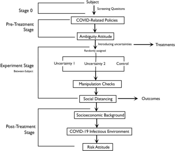
The survey flow
Stage 0
Immediately after accepting our survey invitation, one would then be asked two attention check questions for filtering out perfidious careless respondents (Shamon & Berning, 2020). We then collected the information about our subjects’ age, gender, level of education, and residential area to make sure our final sample could be as similar as Japan’s actual demographics along these dimensions.
Pre-treatment stage
We also asked our respondents various questions about COVID-related policies. They were then followed by a series of Ellsberg (1961)’s two-urn questions to measure one’s attitude towards ambiguity.14 In the literature, it is well known that one’s ambiguity preference is shaped by many factors. For example, it depends on the probability of the risky alternative offered and the outcome domain (e.g., Kocher et al., 2018).
To deal with this issue, we measured ambiguity-attitudes using six different questions involving gain and loss outcomes for both moderate and low likelihood events. For example, the question involving a gain outcome for a moderate event is the following:
Suppose that you pick up a ball from the bag consisting of various color balls. You receive 20,000 yen if you pick up a red ball. Which bag do you prefer?
- A.
Exactly 50% of balls in the bag are red
- B.
The bag consists of red and blue balls, but the exact fraction of red balls is uncertain.
Since B is an ambiguous option, on the one hand, ambiguity-averse (resp. ambiguity-loving) respondents should choose A (resp. B). On the other hand, ambiguity-neutral ones should be indifferent between the two options.15 Summing up the number of times choosing B allows us to construct a measure of ambiguity-attitudes for each subject. Under the assumption that subjects randomly choose either A or B in the indifferent case, ambiguity-neutral ones are expected to choose B three times on average. We therefore coded the ambiguity-averse respondents as those who chose B for two times or less, the ambiguity-neutral ones as those who did so for three times, and the ambiguity-loving ones as those who did so for four times or more.16
What should be noticed here is that they were administered before each subject entered the experiment stage to avoid the post-treatment bias (Montgomery et al., 2018).
Experiment stage
At the experiment stage, all the respondents were randomly assigned to three groups, each of which was provided with a different informational stimulus of the scientific uncertainty surrounding COVID-19. The informational stimuli were then immediately followed by the manipulation check and various questions about respondents’ social distancing decisions. The experiment design will be detailed shortly in Sect. 4.
Post-treatment stage
Finally, to avoid respondent fatigue before the experiment, we left various non-attitudinal survey questions orthogonal to scientific uncertainties to the post-treatment stage. First, we asked respondents’ socioeconomic background and their previous behaviors about COVID-19. At last, we followed Holt and Laury’s (2002) ten paired lottery-choice method to measure subjects’ risk (known probabilities) preferences.
Experimental method and design
Informational treatments
Our experimental design included three groups: Ambiguity 1, Ambiguity 2, and Control. Subjects were randomly assigned to one of them. All subjects read a piece of text (i.e., a vignette) describing the role of science during the COVID-19 outbreak in Japan (see Online Appendix B.1 for both the Japanese vignettes and their English translations). After reading their assigned vignettes, all the respondents were then asked to answer the same set of questions on their perceptions of COVID-19 and preferred levels of preventive behavior.
The vignettes as treatments differ in the nature of scientific (un)certainty in their descriptions. First of all, all the groups were provided with the following plain description about the effective number of reproduction (Re, a measurement of how infectious the virus was) in March estimated by experts with zero ambiguity:
[...] One important scientific reference is the average number of people who become infected by an infectious person (the effective number of reproduction), an important measure of how widespread the virus is. Back in March, this number in Tokyo was estimated by experts to be 2.6. (Experts Meeting on COVID-19 Response, “COVID-19 Response’s Analysis and Advice,” May 1, 2020) In other words, in March, one infected person passed on the virus to 2.6 people, and so on and so forth. The number above indicates how quickly the virus will spread, and it is important to have proper measures.
While the subjects in the Control group then proceed directly to the manipulation checks and social distancing questions, those in both Ambiguity 1 and Ambiguity 2 groups continue to read a few more sentences as informational manipulations that remind them of the uncertain nature of Re.17 Specifically, following the literature of scientific uncertainty (Kreps & Kriner, 2020; Van Der Bles et al., 2020), the respondents of the former read the following information obtained from the same government report:
However, since this number is only an estimate, they also report a possible error and argue that the true number is somewhere between 2.2 and 3.2 with 95% chance. In other words, the number of people one sick person infected in March can either be 2.2 or 3.2 persons.
Since a range of values Re could take would make it harder to mentally formulate the infection rate as a single probability, this vignette attribute help increase the perceived degrees of ambiguity for our subjects. For robustness, we also included the other more intuitive way of inducing ambiguity in Re for the Ambiguity 2 group by utilizing a BBC news article:
On the contrary, since the novel cornonavirus (COVID-19) is a new virus, there is still much these experts do not understand. For example, the answers to the following nine issues are still unknown.
How many people have been infected.
How deadly it really is.
The full range of symptoms.
The role children play in spreading it.
Where exactly it came from.
Whether there will be fewer cases in summer.
Why some people get much more severe symptoms.
How long immunity lasts, and whether you can get it twice.
Whether the virus will mutate.
Compared to the Ambiguity 1 treatment, the one we used for the Ambiguity 2 group did not count on the statistical concept of confidence interval and was not limited to the infection rate to create a sense of ambiguity for our subjects.
Manipulation checks
Before measuring the outcomes of our experiment, respondents’ social distancing decisions, we first checked if the information treatments induce ambiguity in their scientific understanding of COVID-19. Specifically, the following set of questions about the perceived degree of ambiguity (i.e., scientific uncertainty) were asked:
How well do you think scientists know about the nature of COVID-19 and its outbreak?
How well do you think scientists know about the infection rate of the COVID-19?
How well do you think scientists know about the mortality rate of the COVID-19?
Each question uses a 11-point scale (10: no uncertainty, 0: high uncertainty). Since the most important ambiguity regarding the decision of social distancing is the infection rate, in the analysis, we focus on the second question (the effects on the first and third questions are available at Online Appendix.)
Measuring social distancing decisions
Immediately after the manipulation checks, respondents were asked to answer their social distancing decisions and other related questions regarding their preventive behaviors. While we have modeled social distancing as an individual decision-making problem, as a matter of fact, one’s probability of infection can be largely determined by the social context he or she is in. In this sense, the decision of social distancing could actually be strategic, and ambiguity might change one’s decision in response to others’ preventative behaviors.18
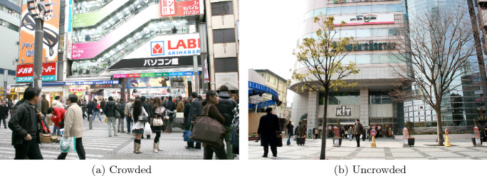
To make the empirical design consistent with our (non-strategic) individual decision-making model, we controlled respondents’ perceived environments by presenting them with two pictures (a, b in Fig. 2) visualizing both crowded and uncrowded situations, and asked the following question for each picture with and without wearing a mask:
Please answer how you would do if a second wave of COVID-19 happens. Suppose you are planning to go to a place with the population density shown in the picture. How likely will you go there during the outbreak of COVID-19 with and without mask?
Each question is a 11-point scale (10: extremely likely, 0: not a chance).19
Fig. 2.
Crowded versus uncrowded situations
All the questions above then constitute four different scenarios in our experiments along two important dimensions in the transmission of the novel coronavirus: (1) crowdedness of a location (high versus low) and (2) mask-wearing (yes versus no). Since our respondents had to make their social distancing decisions in all of them, the setting allows us to estimate the heterogeneous treatment effects across the following four scenarios in Table 1.
Table 1.
Different scenarios
| Crowdedness | Mask-wearing | |
|---|---|---|
| 1 | High | No |
| 2 | High | Yes |
| 3 | Low | No |
| 4 | Low | Yes |
Empirical results
Summary statistics
The effective sample sizes for all experiment conditions and sample balance tests are reported in Appendix B. The balance checks show that there are no systematic differences among them. Since our hypotheses are specific to particular ambiguity attitudes, we also further divided our sample into three sub-samples based on the method specified in Sect. 3.2: ambiguity-averse, ambiguity-neutral, and ambiguity-loving. While they are all quite balanced in almost all the dimensions, the ambiguity-neutral group appears to be unbalanced in gender and education, and this implies that we will have to control for both variables to make sure that the effects we identified are robust.
In addition, Fig. 3 reports the number of subjects for each ambiguity attitude in our sample. Around 50% of subjects are ambiguity-averse, whereas around 25% of subjects are ambiguity-loving. This pattern is consistent with the existing empirical findings (Cavatorta & Schröder, 2019; Dimmock et al., 2015; Kocher et al., 2018) .20 Since the first option (i.e., option A) in each question is an unambiguous option, ambiguity-averse subjects might contain satisficers who chose the first option without reading materials carefully enough. To see if this is the case, Fig. 4 plots the density of response time for each ambiguity-attitude. Since the density is similar across the ambiguity-attitude groups, we don’t have to be worried about this issue.
Fig. 3.
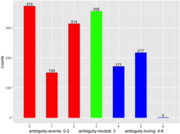
Distribution of ambiguity-attitudes
Fig. 4.
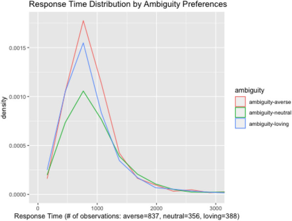
Density plot for response time
Manipulation check: effect on perceived degree of ambiguity
As a manipulation check, we start with examining whether the treatment increased the perceived degree of ambiguity. For this purpose, we estimated the following linear regression model:
| 1 |
where is the outcome, represents the treatment dummy of Ambiguity 1, and represents the treatment dummy of Ambiguity 2. represents that observation i is in the Ambiguity j treatment group, and represents otherwise. If , the observation is in the control group. The coefficient of interest is . A negative implies that the treatment increases the perceived degree of ambiguity compared to the control group. represent the control variables, and is the error term. We estimated this equation with and without controls.
Figure 5 reports the estimated treatment effects on ambiguity regarding the infection rate. Since a higher value represents less ambiguity, on the whole, the findings indicate that the perceived levels of ambiguity in the Ambiguity groups are higher compared to the Control group. That is, our treatment information did increase the perceived degree of ambiguity among our subjects and our manipulation worked.
Fig. 5.
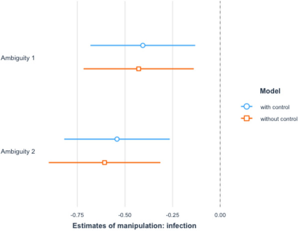
Ambiguity on the infection rate. Notes: We ran OLS with the dummies of Ambiguity 1 and Ambiguity 2 as independent variables and report the estimated coefficients of the two dummy variables
Effect on social distancing
We next report the results on social distancing. To make sure our results are robust across different situations, we asked the willingness to conduct social distancing in four different scenarios along two dimensions in the transmission of the novel coronavirus: (1) crowdedness of a location (high versus low) and (2) mask-wearing (yes versus no). Our respondents had to make their social distancing decisions in all theses cases above.
Pooling results
We start with the aggregated result. To report the pooling results, we estimated the following linear regression model:
| 2 |
is the (un)willingness to social distancing in scenario j, and the higher value implies that a respondent is less willing to take social distancing. We use the clustered standard errors. We estimated this equation with and without controls.
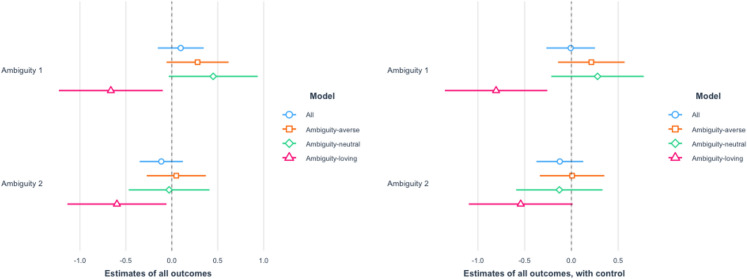
The results are reported in Fig. 6. As in the figure, the treatment has no effect on average. However, this does not imply that the treatment has no influence on respondents’ willingness to take preventive behaviors. As our theory indicates, the effect could be heterogeneous depending on each respondent’s ambiguity-attitude.
Fig. 6.
Aggregated effect for all outcomes. We ran OLS with the dummies of Ambiguity 1 and Ambiguity 2 as independent variables and report the estimated coefficients of the two dummy variables. The left panel shows the result of OLS without controls, whereas the right panel shows the result of OLS with controls
To see whether this is the case, we estimated (2) for each subgroup (ambiguity-loving respondents, ambiguity-neutral respondents, and ambiguity-averse respondents). The results are also reported in Fig. 6. As they show, the findings are consistent with our Hypothesis 2 and robust with additional controls. That is, our treatment increases ambiguity-loving respondents’ level of social distancing. In contrast, there is no such relationship among the ambiguity-averse and ambiguity-neutral ones. In particular, for Ambiguity 1 group, the treatment decreases the level of social distancing among them, while they are not statistically significant.
While this result seems to be puzzling at first glance, it can be understood as follows. Let us take whether one’s family members are infected as an example of the determinants of infection. Regardless of social distancing, one will be infected once his or her family members are infected. Thus, the effectiveness of social distancing is increasing in the likelihood of the family members not being infected. In the presence of higher ambiguity, this likelihood becomes more uncertain. For ambiguity-loving people who are optimistic, this implies that their family members are less likely to be infected; thus their perceived effectiveness of social distancing increases, which induces social distancing. On the other hand, for ambiguity-averse people who are pessimistic, this implies that the family members are more likely to be infected; thus their perceived effectiveness of social distancing decreases, which reduces social distancing. This is (ii) in Proposition 1, and our result is consistent with this prediction.
Individual scenarios
To see whether this identified effect is robust across different scenarios, we estimated the following linear regression model for each scenario:
| 3 |
where is the (un)willingness to social distancing in a scenario. We estimated this equation with and without controls.
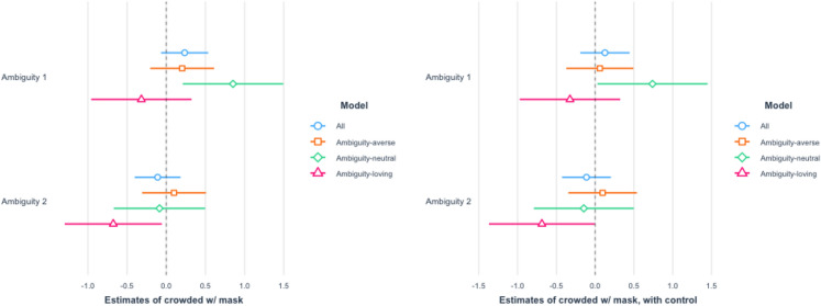
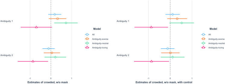
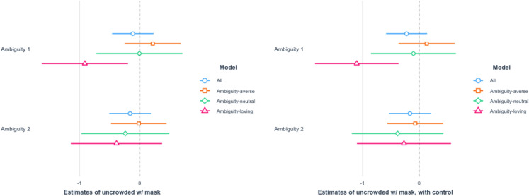
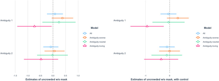
The results for the high crowdedness are reported in Figs. 7 and 8. The effects on ambiguity-loving respondents are statistically significant for the Ambiguity 2 treatment in the high crowdedness scenarios. The results for the low crowdedness are reported in Figs. 9 and 10. In these cases, the effects on ambiguity-loving respondents are statistically significant for the Ambiguity 1 treatment. While which of the two treatment arms is effective differs across scenarios, the findings are consistent with Hypothesis 2.
Fig. 7.
Crowded place with a mask put on The left panel shows the result of OLS without controls, whereas the right panel shows the result of OLS with controls
Fig. 8.
Crowded place without a mask put on. The left panel shows the result of OLS without controls, whereas the right panel shows the result of OLS with controls
Fig. 9.
Uncrowded place with a mask put on. We ran OLS with the dummies of Ambiguity 1 and Ambiguity 2 as independent variables and report the estimated coefficients of the two dummy variables. The left panel shows the result of OLS without controls, whereas the right panel shows the result of OLS with controls
Fig. 10.
Uncrowded place without a mask put on. We ran OLS with the dummies of Ambiguity 1 and Ambiguity 2 as independent variables and report the estimated coefficients of the two dummy variables. The left panel shows the result of OLS without controls, whereas the right panel shows the result of OLS with controls
Overall, the effect of ambiguity is heterogeneous depending on ambiguity-attitudes, and it encourages ambiguity-loving subjects to increase the level of social distancing. Furthermore, these findings are robust across different scenarios.
As for the magnitude, our findings are also fairly substantial. For the scenario of going to a crowded place without wearing a mask, ambiguity-loving respondents were almost 20% (23% for Ambiguity 1 and 20% for Ambiguity 2) less likely to visit a place.21 The percentage went down a bit to near 10-20% with a mask worn (11% for Ambiguity 1 and 23% for Ambiguity 2). As for the less dangerous situation of an almost empty place, the effect is still substantial. For an uncrowded place like Fig. 2b, respondents were 10–20% less likely to keep social distance even with a mask put on (21% for Ambiguity 1 and 9% for Ambiguity 2). The percentage went up a little to 20–30% (30% for Ambiguity 1 and 19% for Ambiguity 2) when no mask was worn.
While the empirical patterns are consistent with our Hypothesis 2, it should be noted that there are still some discrepancies between our theoretical framework and empirical findings. First, our model also predicts that ambiguity-loving agents are more likely to take preventive behaviors than ambiguity-averse ones when b(k, e) is increasing in k. However, according to our regression analysis, the comparison between ambiguity-averse and ambiguity-loving agents in the Control group shows the opposite (see Online Appendix A). Since ambiguity-attitudes are correlated with other factors, this comparison within the Control group has no causal significance, but it should be noted.22
Another discrepancy is about the effect on ambiguity-averse agents. Though we have focused on the ambiguity-loving subjects, our theory also predicts that higher ambiguity reduces social distancing among the ambiguity-averse agents when b(k, e) is increasing in k. The results for ambiguity-averse respondents are consistent with this prediction, but the effect size is smaller than that of ambiguity-loving counterparts.23 Explaining these discrepancies will be our future work.
Conclusion
This paper studies how people make decisions over preventive behaviors under ambiguity (i.e., Knightian uncertainty) where they do not even know the probability of a loss. Scientific uncertainty makes it difficult to evaluate the current COVID-19 situation based on a single probability—e.g., ambiguity regarding its infection rate. As a result, the outbreak of COVID-19 gives us an exceptional opportunity for empirically analyzing the effect of ambiguity on preventive behaviors.
Our theoretical model shows how its effect is heterogeneous depending on ambiguity-attitudes. In particular, higher ambiguity induces only ambiguity-loving agents’ social distancing when the marginal effectiveness of social distancing and the probability of infection are negatively correlated. Motivated by this theory, we conducted a survey experiment in Japan. In the experiment, we manipulated the information regarding the scientific uncertainty on COVID-19. We found that higher ambiguity increased the level of social distancing among the ambiguity-loving respondents, while such an effect was nonexistent for ambiguity-averse counterparts. In short, higher ambiguity has a heterogeneous effect on preventive behaviors, depending on ambiguity-attitudes.
Our results have two implications for the risk communication strategy of governments and experts. First, they should take this heterogeneous effect into account when communicating scientific uncertainty to the public. Since the effect is heterogeneous, risk communication would be more effective if governments have sufficient information on individual heterogeneous ambiguity-attitudes and can design risk communication customarily to each individual. Second, the risk communication strategy should be mainly designed to promote the transparency in disease information. While transparency might introduce more ambiguity regarding the virus among people, it has been shown to enhance the government credibility (Porat et al., 2020; Sheen et al., 2021), which is critical to facilitating the public’s cooperation during a public health crisis. On top of this, our study shows that it has the benefit of making ambiguity-loving people, who are typically regarded as not taking preventive measures, keep social distance. These insights indicate that promoting the transparency is an appropriate risk communication strategy.
Despite the prevalence of ambiguity in daily decisions, this paper is the first attempt to do a rigorous empirical test with a randomized experiment. While it was conducted in a specific context of social distancing amid the COVID-19 outbreak, the implications of our findings can also be readily extended to other contexts of scientific uncertainty. For example, the concept of (scientific) ambiguity has also been applied to the issue of climate change (Millner et al., 2013; Lemoine & Traeger, 2016) where its science has been subject to intensive debates and contested conclusions. Our analytic framework and the empirical finding about ambiguity-lovers’ self-protective behaviors could be extended to such context.
Supplementary Information
Below is the link to the electronic supplementary material.
Appendix
-
A
Proof of Proposition 1
-
B
Sample Balance Tests
A Proof of Proposition 1
-
(i)Since b is decreasing in k, is the best case for the individual, whereas is the worst case. Hence,
By taking the first-order condition, we have
where24
Hence, by applying the implicit function theorem, we have
Since and the denominator is negative, this implies that
Here, (resp. ) is decreasing (resp. increasing) in . Thus, when is close to one, , while when is close to zero. This completes the proof. -
(ii)In this case, is the best case for the individual, whereas is the worst case. Hence,
Given this, as in (i), we obtain the proposition.
B Sample balance tests
Table 2.
Summary statistics and balance checks
| Summary statistics and balance check: all samples | ||||||
|---|---|---|---|---|---|---|
| Variable | N | Overall, | Ambiguity 1, | Ambiguity 2, | Control, | p value |
| Female | 1581 | 790 (50%) | 266 (50%) | 259 (49%) | 265 (51%) | 0.88 |
| Age | 1581 | 52 (40,69) | 51 (39, 68) | 52 (41, 66) | 54 (40,70) | 0.44 |
| College | 1581 | 368 (23%) | 121 (23%) | 133 (25%) | 114 (22%) | 0.40 |
| Highschool | 1581 | 633 (40%) | 216 (41%) | 201 (38%) | 216 (41%) | 0.54 |
| Junior college | 1581 | 180 (11%) | 49 (9.2%) | 62 (12%) | 69 (13%) | 0.12 |
| Vocational school | 1581 | 103 (6.5%) | 39 (7.3%) | 33 (6.3%) | 31 (5.9%) | 0.62 |
| Income | 1359 | 0.54 | ||||
| 99.5 | 174 (13%) | 67 (15%) | 50 (11%) | 57 (13%) | ||
| 299.5 | 387 (28%) | 117 (25%) | 130 (29%) | 140 (31%) | ||
| 499.5 | 318 (23%) | 122 (27%) | 100 (22%) | 96 (21%) | ||
| 699.5 | 202 (15%) | 67 (15%) | 74 (17%) | 61 (13%) | ||
| 899.5 | 132 (9.7%) | 39 (8.5%) | 47 (11%) | 46 (10%) | ||
| 1099.5 | 51 (3.8%) | 15 (3.3%) | 16 (3.6%) | 20 (4.4%) | ||
| 1299.5 | 43 (3.2 %) | 17 (3.7%) | 11 (2.5%) | 15 (3.3%) | ||
| 1400 | 52 (3.8%) | 15 (3.3%) | 18 (4.0%) | 19 (4.2%) | ||
| Unknown | 222 | 72 | 81 | 69 | ||
| Ambiguity averse | 1581 | 837 (53%) | 282 (53%) | 291 (55%) | 264 (50%) | 0.30 |
| Ambiguity neutral | 1581 | 356 (23%) | 117 (22%) | 106 (20%) | 133 (25%) | 0.11 |
| Ambiguity loving | 1581 | 388 (25%) | 132 (25%) | 130 (25%) | 126 (24%) | 0.96 |
n (%); median (IQR)
Pearson’s Chi-squared test; Kruskal-Wallis rank sum test
Table 3.
Summary statistics and balance checks: ambiguity-averse samples
| Summary statistics and balance check: ambiguity-averse samples | ||||||
|---|---|---|---|---|---|---|
| Variable | N | Overall, | Ambiguity 1, | Ambiguity 2, | Control, | p value |
| Female | 837 | 389 (46%) | 140 (50%) | 129 (44%) | 120 (45%) | 0.41 |
| Age | 837 | 52 (40,66) | 50 (39,66) | 52 (40,64) | 54 (40,69) | 0.52 |
| College | 837 | 221 (26%) | 64 (23%) | 86 (30%) | 71 (27%) | 0.17 |
| Highschool | 837 | 315 (38%) | 113 (40%) | 104 (36%) | 98 (37%) | 0.55 |
| Junior college | 837 | 95 (11%) | 23 (8.2%) | 34 (12%) | 38 (14%) | 0.070 |
| Vocational school | 837 | 63 (7.5%) | 28 (9.9%) | 15 (5.2%) | 20 (7.6%) | 0.10 |
| Income | 728 | 0.41 | ||||
| 99.5 | 90 (12%) | 37 (15%) | 29 (11%) | 24 (10%) | ||
| 299.5 | 192 (26%) | 51 (21%) | 68 (27%) | 73 (32%) | ||
| 499.5 | 167 (23%) | 64 (26%) | 58 (23%) | 45 (19%) | ||
| 699.5 | 112 (15%) | 38 (16%) | 40 (16%) | 34 (15%) | ||
| 899.5 | 85 (12%) | 28 (12%) | 32 (13%) | 25 (11%) | ||
| 1099.5 | 30 (4.1%) | 6 (2.5%) | 10 (3.9%) | 14 (6.1%) | ||
| 1299.5 | 22 (3.0%) | 8 (3.3%) | 8 (3.1%) | 6 (2.6%) | ||
| 1400 | 30 (4.1%) | 10 (4.1%) | 10 (3.9%) | 10 (4.3%) | ||
| Unknown | 109 | 40 | 36 | 33 | ||
n (%); median (IQR)
Pearson’s Chi-squared test; Kruskal-Wallis rank sum test
Table 4.
Summary statistics and balance checks: ambiguity-neutral samples
| Summary statistics and balance check: ambiguity-neutral samples | ||||||
|---|---|---|---|---|---|---|
| Variable | N | Overall, | Ambiguity 1, | Ambiguity 2, | Control, | p value |
| Female | 356 | 190 (53%) | 50 (43%) | 63 (59%) | 77 (58%) | 0.019 |
| Age | 356 | 59 (39,71) | 50 (36, 70) | 53 (41,71) | 56 (39,71) | 0.57 |
| College | 356 | 70 (20%) | 28 (24%) | 19 (18%) | 23 (17%) | 0.36 |
| Highschool | 356 | 161 (45%) | 48 (41%) | 46 (43%) | 67 (50%) | 0.30 |
| Junior college | 356 | 33 (9.3%) | 5 (4.3%) | 12 (11%) | 16 (12%) | 0.074 |
| Vocational school | 356 | 19 (5.3%) | 7 (6.0%) | 6 (5.7%) | 6 (4.5%) | 0.86 |
| Income | 315 | |||||
| 99.5 | 39 (12%) | 12 (11%) | 12 (13%) | 15 (13%) | ||
| 299.5 | 103 (33%) | 38 (36%) | 31 (35%) | 34 (29%) | ||
| 499.5 | 80 (25%) | 31 (29%) | 19 (21%) | 30 (35%) | ||
| 699.5 | 33 (10%) | 11 (10%) | 10 (11%) | 12 (10%) | ||
| 899.5 | 33 (10%) | 8 (7.5%) | 11 (12%) | 14 (12%) | ||
| 1099.5 | 9 (2.9%) | 4 (3.7%) | 2 (2.2%) | 3 (2.5%) | ||
| 1299.5 | 7 (2.2%) | 1 (0.9%) | 1 (1.1%) | 5 (4.2%) | ||
| 1400 | 11 (3.5%) | 2 (1.9%) | 3 (3.4%) | 6 (5.0%) | ||
| Unknown | 41 | 10 | 17 | 14 | ||
n (%); median (IQR)
Pearson’s Chi-squared test; Kruskal-Wallis rank sum test
Table 5.
Summary statistics and balance checks: ambiguity-loving samples
| Summary statistics and balance check: ambiguity-loving samples | ||||||
|---|---|---|---|---|---|---|
| Variable | N | Overall, | Ambiguity 1, | Ambiguity 2, | Control, | p value |
| Female | 388 | 211 (54%) | 76 (58%) | 67 (52%) | 68 (54%) | 0.61 |
| Age | 388 | 52 (40,70) | 55 (39,70) | 50 (40, 70) | 52 (40, 71) | 0.96 |
| College | 388 | 77 (20%) | 29 (22%) | 28 (22%) | 20 (16%) | 0.39 |
| Highschool | 388 | 157 (40%) | 55 (42%) | 51 (39%) | 51 (40%) | 0.92 |
| Junior college | 388 | 52 (13%) | 21 (16%) | 16 (12%) | 15 (12%) | 0.58 |
| Vocational school | 388 | 21 (5.4%) | 4 (3.0%) | 12 (9.2%) | 5 (4.0%) | 0.058 |
| Income | 316 | |||||
| 99.5 | 45 (14%) | 18 (16%) | 9 (8.8%) | 18 (17%) | ||
| 299.5 | 92 (29%) | 28 (25%) | 31 (30%) | 33 (32%) | ||
| 499.5 | 71 (22%) | 27 (25%) | 23 (23%) | 21 (20%) | ||
| 699.5 | 57 (18%) | 18 (16%) | 24 (24%) | 15 (14%) | ||
| 899.5 | 14 (4.4%) | 3 (2.7%) | 4 (3.9%) | 7 (6.7%) | ||
| 1099.5 | 12 (3.8%) | 5 (4.5%) | 4 (3.9%) | 3 (2.9%) | ||
| 1299.5 | 14 (4.4%) | 8 (7.3%) | 2 (2.0%) | 4 (3.8%) | ||
| 1400 | 11 (3.5%) | 3 (2.7%) | 5 (4.9%) | 3 (2.9%) | ||
| Unknown | 72 | 22 | 28 | 22 | ||
n (%); median (IQR)
Pearson’s Chi-squared test; Kruskal-Wallis rank sum test
Footnotes
Siobhan Roberts. Embracing the Uncertainties. New York Times, April 7, 2020. https://www.nytimes.com/2020/04/07/science/coronavirus-uncertainty-scientific-trust.html?auth=login-google. Accessed August 20, 2022.
Several other studies also conduct online surveys on COVID-19 preventive behavior in Japan (e.g., Cato et al., 2020; Ikeda et al., 2020; Muto et al., 2020; Stickley et al., 2020).
Millner et al. (2013) also consider a similar issue in the specific context of climate change.
In addition, several studies analyze how the outbreak of COVID-19 changes people’s risk preferences (Bu et al., 2020; Ikeda et al., 2020).
For simplicity, we only focus on the probability of infection in the model. However, it can be easily extended to a situation where other probabilities matter. For example, if we relabel I as the state of death, can be interpreted as the mortality rate.
Another possible specification is that . Here, is a candidate of the true probability. An individual thinks that is true with probability , whereas, is wrong and any distribution can be true with the another probability. This specification is called the Choquet expected utility with a neo-additive capacity. Differently from our hypotheses, this setting predicts that higher ambiguity reduces preventive behaviors independently of ambiguity-attitudes (Teitelbaum, 2007). This prediction is inconsistent with the empirical patterns we found.
-Maxmin expected utility theory does not necessarily allow agents to be ambiguity-neutral, and thus our theoretical prediction does not include the effect on ambiguity-neutral agents. While this is the case, the effect on ambiguity-neutral agents should be zero by definition.
With an additional parametric assumption on b(k, e), we can additionally prove the threshold property: is decreasing in if and only if .
An example is the following functional form: .
An example is the following functional form: .
While 1581 respondents finished the survey, some of them chose “don’t know” or skip the answer for some questions, which causes some missing variables for some questions.
The first wave of the outbreak took place in Japan in March and lasted for about two months. On April 7, a state of emergency was declared for seven prefectures including Tokyo, and expanded to the entire country on April 16. After the number of infections was substantially reduced, the Japanese government lifted the state of emergency on May 25. In early July, however, Japan faced the second wave, whose peak was reached at the end of the same month. During the second wave, the government did not declare a state of emergency and our survey was conducted right at the beginning of the second wave.
See Online Appendix D for the English translation of the full questionnaire. The original Japanese version is also available upon request.
Similar questions are often used to measure the degree of ambiguity-aversion/loving. In particular, Kocher et al. (2018) use a similar set of questions to measure ambiguity-attitudes in their first stage analysis. Note that many studies measuring ambiguity-attitudes are based on incentivized experiments (e.g., Kocher et al. 2018), whereas ours are thought experiments in a survey module. Cavatorta and Schröder (2019) find that an appropriate survey module, just like an incentivized experiment, can also yield predictions about ambiguity-attitudes.
In the framework of Maxmin expected utility theory, a subject strictly prefers A to B if and only if s/he is given that the subject recognizes the existence of ambiguity (see Dimmock et al., 2015, Section 3.4).
Another way to measure ambiguity-attitudes is to monotonically change the probability of winning a prize in the risky urn and identify the switching point (e.g., Dimmock et al., 2015; Kocher et al., 2018; Cavatorta & Schröeder, 2019). For example, in the above question, by monotonically changing the percentage of red balls in A, we can identify the percentage of red balls in A, where a subject is indifferent between the two options. Although this approach enables us to measure the precise degree of ambiguity-attitudes, it forces subjects to answer a lot of questions in addition to those regrading COVID-19. Since this is not very feasible, we adopted the current approach.
The Control group receives information that Re was estimated to be 2.6, which may work as an anchor for subjects’ decision-making. While this is the case, in a vignette design, the remaining part of the information stimulus except the treatment information needs to be as close as possible between the control and the treatment groups. For this purpose, we need to provide information about the estimated number of Re to the control group as well as the treatment groups. Since all the three groups shared the same anchor about the value of Re and the control group received no information about scientific uncertainty, the differences in respondents’ answers regarding their social distancing decisions between the treatment and the control groups is the causal effect of the information about scientific uncertainty.
See, for example, Kishishita and Ozaki (2020) for theoretical predictions about the effect of ambiguity on strategic interactions. In an experiment, Vives and FeldmanHall (2018) find that one’s ambiguity-attitude affects his or her belief on others’ pro-social behaviors, which in turn affects his or her pro-social behavior.
The situation asked in the question was not so realistic given the limited testing scheme the Japanese government adopted at that time. Thus, we do not use the answers for these question. The results for this question is available at Online Appendix.Suppose all the people in the picture above have tested negative for the virus. How likely will you go there during the outbreak of the COVID-19 with and without mask?
While we simply summed up the number of times choosing an ambiguous option, it has been found that one’s ambiguity-attitude tends to be asymmetric between a gain and loss domain as the prospect theory suggests (e.g., Kocher et al., 2018). This regularity found in the literature is also supported by our data. On average, people tend to choose an ambiguous option for loss outcomes rather than gain outcomes (Online Appendix A.2). It should be noted that our simple measurement does not incorporate such asymmetry because it does not distinguish between gain and loss outcomes. Having said this, except for the gain domain with 50% chance, subjects classified as being ambiguity-loving choose an ambiguous option regardless of its domain (Online Appendix A.2). Similarly, subjects classified as being ambiguity-averse choose an unambiguous option regardless of its domain. Hence, the gain-loss asymmetry does not influence ambiguity-attitudes much at least among subjects being classified as being ambiguity-loving or ambiguity-averse. On the other hand, attitudes of subjects classified as being ambiguity-neutral depend on whether outcomes are gains or losses.
This number is calculated as follows based on the regression table available at Online Appendix. Based on the regression without controls, the average for the control group is 2.252, while the average for the Ambiguity 1 group is 1.556. Based on these numbers, the effect size is calculated as .
This discrepancy can be resolved by introducing heterogeneous beliefs on V(I): if ambiguity-averse agents are pessimistic about the value of V(I), their baseline level of social distancing is high. Another potential mechanism is that more ambiguity increases social distancing independently of ambiguity-attitudes, but its effect is weak for ambiguity-averse people because their level of preventive behaviors is already high. However, it is inconsistent with our finding that the treatment sometimes discourages social distancing.
For some outcomes, the treatment effect is statistically significant among ambiguity-neutral subjects. We classified those who chose option B three times in Ellsberg’s urn experiments as ambiguity-neutral subjects, but this classification does not guarantee that the subjects are literally ambiguity-neutral. For example, a subject choosing option A for all the gain domain questions and choosing option B for all the loss domain questions is classified as ambiguity-neutral. However, a more appropriate interpretation is that the subject was ambiguity-averse in the gain domain, while he or she is ambiguity-loving in the loss domain. Consequently, the subjects might contain a mixture of ambiguity-averse and ambiguity-loving agents. This could be a source of the non-zero treatment effect among ambiguity-neutral subjects.
from the assumption that . Furthermore, is assumed. Hence, the second-order condition is trivially satisfied.
The survey was approved by the Institutional Review Boards at both Columbia University (AAAT0545) and National Taiwan University (202005HS103), and pre-registered at the AEA RCT Registry (AEARCTR-0006115). The research was funded by Taiwan’s Ministry of Education (109L8923) and Japan Society for the Promotion of Science (20K22131). The authors would like to thank Takanori Ida (a co-editor), the anonymous referee, Shohei Yanagita, seminar participants at Waseda University, and participants of the 2021 Annual Meeting of the Association of Behavioral Economics and Finance at Seijo University for their helpful comments.
Publisher's Note
Springer Nature remains neutral with regard to jurisdictional claims in published maps and institutional affiliations.
Contributor Information
Daiki Kishishita, Email: daiki.kishishita@gmail.com.
Hans H. Tung, Email: hanstung@ntu.edu.tw
Charlotte Wang, Email: cw3204@columbia.edu.
References
- Alary D, Gollier C, Treich N. The effect of ambiguity aversion on insurance and self-protection. The Economic Journal. 2013;123(573):1188–1202. doi: 10.1111/ecoj.12035. [DOI] [Google Scholar]
- Alesina A, Stantcheva S, Teso E. Intergenerational mobility and preferences for redistribution. American Economic Review. 2018;108(2):521–554. doi: 10.1257/aer.20162015. [DOI] [Google Scholar]
- Bu, D., Hanspal, T., Liao, Y., & Liu, Y. (2020). Economic preferences during a global crisis: Evidence from Wuhan. Available at SSRN 3559870.
- Cato, S., Iida, T., Ishida, K., Ito, A., McElwain, K. M., & Shoji, M. (2020). Social distancing as a public good under the COVID-19 pandemic. Public Health, (Forthcoming). [DOI] [PMC free article] [PubMed]
- Cavatorta E, Schröder D. Measuring ambiguity preferences: A new ambiguity preference survey module. Journal of Risk and Uncertainty. 2019;58(1):71–100. doi: 10.1007/s11166-019-09299-0. [DOI] [Google Scholar]
- Chiu WH. On the propensity to self-protect. Journal of Risk and Insurance. 2000;67:555–577. doi: 10.2307/253850. [DOI] [Google Scholar]
- Dimmock SG, Kouwenberg R, Mitchell OS, Peijnenburg K. Estimating ambiguity preferences and perceptions in multiple prior models: Evidence from the field. Journal of Risk and Uncertainty. 2015;51(3):219–244. doi: 10.1007/s11166-015-9227-2. [DOI] [PMC free article] [PubMed] [Google Scholar]
- Eeckhoudt L, Gollier C. The impact of prudence on optimal prevention. Economic Theory. 2005;26(4):989–994. doi: 10.1007/s00199-004-0548-7. [DOI] [Google Scholar]
- Ellsberg, D. (1961). Risk, ambiguity, and the Savage axioms. The Quarterly Journal of Economics, 75, 643–669.
- Han PK, Zikmund-Fisher BJ, Duarte CW, Knaus M, Black A, Scherer AM, Fagerlin A. Communication of scientific uncertainty about a novel pandemic health threat: Ambiguity aversion and its mechanisms. Journal of Health Communication. 2018;23(5):435–444. doi: 10.1080/10810730.2018.1461961. [DOI] [PMC free article] [PubMed] [Google Scholar]
- Holt CA, Laury SK. Risk Aversion and Incentive Effects. American Economic Review. 2002;92(5):1644–1655. doi: 10.1257/000282802762024700. [DOI] [Google Scholar]
- Hurwicz L. Some specification problems and applications to econometric models. Econometrica. 1951;19(3):343–344. [Google Scholar]
- Ikeda S, Yamamura E, Tsutsui Y. COVID-19 enhanced diminishing sensitivity in prospect-theory risk preferences: A panel analysis. Institute of Social and Economic Research Discussion Papers. 2020;1106:1–25. [Google Scholar]
- Insight R. Panel Book 2020. Rakuten Insight; 2020. [Google Scholar]
- Johnson BB, Slovic P. Presenting uncertainty in health risk assessment: Initial studies of its effects on risk perception and trust. Risk Analysis. 1995;15(4):485–494. doi: 10.1111/j.1539-6924.1995.tb00341.x. [DOI] [PubMed] [Google Scholar]
- Karadja M, Mollerstrom J, Seim D. Richer (and Holier) than thou? The effect of relative income improvements on demand for redistribution. Review of Economics and Statistics. 2017;99(2):201–212. doi: 10.1162/REST_a_00623. [DOI] [Google Scholar]
- Kishishita D, Ozaki H. Public goods game with ambiguous threshold. Economics Letters. 2020;191:109165. doi: 10.1016/j.econlet.2020.109165. [DOI] [Google Scholar]
- Klibanoff P, Marinacci M, Mukerji S. A smooth model of decision making under ambiguity. Econometrica. 2005;73(6):1849–1892. doi: 10.1111/j.1468-0262.2005.00640.x. [DOI] [Google Scholar]
- Kocher MG, Lahno AM, Trautmann ST. Ambiguity aversion is not universal. European Economic Review. 2018;101:268–283. doi: 10.1016/j.euroecorev.2017.09.016. [DOI] [Google Scholar]
- Kreps SE, Kriner DL. Model uncertainty, political contestation, and public trust in science: Evidence from the COVID-19 pandemic. Science Advances. 2020;6(43):eabd4563. doi: 10.1126/sciadv.abd4563. [DOI] [PMC free article] [PubMed] [Google Scholar]
- Kuziemko I, Buell RW, Reich T, Norton MI. “Last-place Aversion”: Evidence and redistributive implications. The Quarterly Journal of Economics. 2014;129(1):105–149. doi: 10.1093/qje/qjt035. [DOI] [Google Scholar]
- Kuziemko I, Norton MI, Saez E, Stantcheva S. How elastic are preferences for redistribution? Evidence from randomized survey experiments. American Economic Review. 2015;105(4):1478–1508. doi: 10.1257/aer.20130360. [DOI] [Google Scholar]
- Lemoine D, Traeger CP. Ambiguous tipping points. Journal of Economic Behavior & Organization. 2016;132:5–18. doi: 10.1016/j.jebo.2016.03.009. [DOI] [PMC free article] [PubMed] [Google Scholar]
- Miles S, Frewer LJ. Public perception of scientific uncertainty in relation to food hazards. Journal of Risk Research. 2003;6(3):267–283. doi: 10.1080/1366987032000088883. [DOI] [Google Scholar]
- Millner A, Dietz S, Heal G. Scientific ambiguity and climate policy. Environmental and Resource Economics. 2013;55(1):21–46. doi: 10.1007/s10640-012-9612-0. [DOI] [Google Scholar]
- Montgomery JM, Nyhan B, Torres M. How conditioning on posttreatment variables can ruin your experiment and what to do about it. American Journal of Political Science. 2018;62(3):760–775. doi: 10.1111/ajps.12357. [DOI] [Google Scholar]
- Muto K, Yamamoto I, Nagasu M, Tanaka M, Wada K. Japanese citizens’ behavioral changes and preparedness against COVID-19: An online survey during the early phase of the pandemic. PLoS One. 2020;15(6):e0234292. doi: 10.1371/journal.pone.0234292. [DOI] [PMC free article] [PubMed] [Google Scholar]
- Peter R. Optimal self-protection in two periods: On the role of endogenous saving. Journal of Economic Behavior & Organization. 2017;137:19–36. doi: 10.1016/j.jebo.2017.01.017. [DOI] [Google Scholar]
- Porat T, Nyrup R, Calvo RA, Paudyal P, Ford E. Public health and risk communication during COVID-19-enhancing psychological needs to promote sustainable behavior change. Frontiers in Public Health. 2020;8:1–15. doi: 10.3389/fpubh.2020.573397. [DOI] [PMC free article] [PubMed] [Google Scholar]
- Shamon H, Berning C. Attention check items and instructions in online surveys with incentivized and non-incentivized samples: Boon or bane for data quality? Survey Research Methods. 2020;14(1):55–77. [Google Scholar]
- Sheen G, Tung HH, Wen-chin W. Citizen journalism reduces the credibility deficit of authoritarian government in risk communication amid COVID-19 outbreaks. PLoS One. 2021;16(12):e0260961. doi: 10.1371/journal.pone.0260961. [DOI] [PMC free article] [PubMed] [Google Scholar]
- Snow A. Ambiguity aversion and the propensities for self-insurance and self-protection. Journal of Risk and Uncertainty. 2011;42(1):27–43. doi: 10.1007/s11166-010-9112-y. [DOI] [Google Scholar]
- Stickley, A., Matsubayashi, T., Sueki, H., & Ueda, M. (2020). COVID-19 preventive behaviors among people with anxiety and depression: Findings from Japan. medRxiv. [DOI] [PMC free article] [PubMed]
- Teitelbaum JC. A unilateral accident model under ambiguity. The Journal of Legal Studies. 2007;36(2):431–477. doi: 10.1086/511895. [DOI] [Google Scholar]
- Van Der Bles AM, van der Linden S, Freeman AL, Spiegelhalter DJ. The effects of communicating uncertainty on public trust in facts and numbers. Proceedings of the National Academy of Sciences. 2020;117(14):7672–7683. doi: 10.1073/pnas.1913678117. [DOI] [PMC free article] [PubMed] [Google Scholar]
- Vives ML, FeldmanHall O. Tolerance to ambiguous uncertainty predicts prosocial behavior. Nature Communications. 2018;9(1):1–9. doi: 10.1038/s41467-018-04631-9. [DOI] [PMC free article] [PubMed] [Google Scholar]
- Weinzierl M. Revisiting the classical view of benefit-based taxation. Economic Journal. 2018;128(612):37–64. doi: 10.1111/ecoj.12462. [DOI] [Google Scholar]
Associated Data
This section collects any data citations, data availability statements, or supplementary materials included in this article.


