Artificial intelligence strategy integrating morphologic and architectural biomarkers provides robust diagnostic accuracy for disease progression in chronic lymphocytic leukemia

Abstract

Artificial intelligence-based tools designed to assist in the diagnosis of lymphoid neoplasms remain limited. The development of such tools can add value as a diagnostic aid in the evaluation of tissue samples involved by lymphoma. A common diagnostic question is the determination of chronic lymphocytic leukemia (CLL) progression to accelerated CLL (aCLL) or transformation to diffuse large B-cell lymphoma (Richter transformation; RT) in patients who develop progressive disease. The morphologic assessment of CLL, aCLL, and RT can be diagnostically challenging. Using established diagnostic criteria of CLL progression/transformation, we designed four artificial intelligence-constructed biomarkers based on cytologic (nuclear size and nuclear intensity) and architectural (cellular density and cell to nearest-neighbor distance) features. We analyzed the predictive value of implementing these biomarkers individually and then in an iterative sequential manner to distinguish tissue samples with CLL, aCLL, and RT. Our model, based on these four morphologic biomarker attributes, achieved a robust analytic accuracy. This study suggests that biomarkers identified using artificial intelligence-based tools can be used to assist in the diagnostic evaluation of tissue samples from patients with CLL who develop aggressive disease features.

Introduction

Deep learning algorithms have been applied on digital pathology images to improve diagnostic accuracy and correlate with biologic subsets [1–5]. Limited studies have described deep learning algorithms to evaluate lymphoid proliferations, and their main focus has been to distinguish benign from malignant conditions [6–11] and different subtypes of lymphoma [9,10,12]. Most studies have adopted a patch-wise strategy for whole-slide image analysis, which entails making diagnostic predictions for patches using a convolutional neural network (CNN) followed by fusing patch predictions to render a final slide diagnosis. The main limitation of this deep learning model is the lack of clinical relatability, as using CNNs derives uninterpretable features from patches without a systematic stepwise approach of disease-specific feature identification.

Artificial intelligence (AI) models used to date to evaluate lymphocytic proliferations remain limited. Meanwhile, several persistent and clinically relevant areas of diagnostic overlap in the evaluation of lymphomas in tissue samples exist and can benefit from machine-assisted diagnostic evaluation. We hypothesized that generating patterns integrating cell morphologic traits (nuclear size and nuclear intensity) and spatial patterns (cellular density and cell to nearest-neighbor cell distance) would be uniquely suited for enhancing the diagnostic accuracy of lymphoid neoplasms.

To test our hypothesis and develop our model, we used chronic lymphocytic leukemia (CLL) as a disease prototype, as it is among the most common lymphoid neoplasms in adults. In addition, CLL is known to undergo stepwise progression to aggressive disease. Typical CLL comprises monomorphous sheets of small, mature lymphocytes interspersed by areas termed ‘proliferation centers’ containing larger cells that include prolymphocytes and large cells referred to as paraimmunoblasts. CLL is generally an indolent disease, although in ~10% of patients it can undergo transformation to a more clinically aggressive variant, most commonly diffuse large B-cell lymphoma (DLBCL) [13]. This phenomenon is termed Richter transformation (RT). An intermediate stage of progression, termed accelerated phase CLL (aCLL), demonstrates overlapping clinical and morphologic features of both CLL and RT [14]. The morphologic assessment of CLL, aCLL, and RT can be diagnostically challenging, particularly in small needle core biopsy specimens. We thought that this stepwise progression model of CLL, aCLL, and RT would be an ideal substrate to test our hypothesis and refine an AI model.

We demonstrate herein that the sequential implementation of key morphologic biomarkers including nuclear size, nuclear intensity, cellular density, and cell to nearest-neighbor distance improved incrementally the accuracy of assessing CLL, aCLL, and RT.

Materials and methods

Study design

The study design is shown in Figure 1 and is detailed below. In brief, we collected and analyzed digital slides of patients diagnosed with at least one of the following entities: CLL, aCLL, and/or RT. Starting with digitized whole-slide images (WSI), we manually selected regions of interest (ROI) (Figure 1A) and then applied stain normalization (Figure 1B) followed by nuclear segmentation (Figure 1C) to delineate nuclei. We used nuclear filtering (Figure 1D) to exclude overlapping nuclei. We characterized each ROI through quantification of nuclear size (Figure 1E) and nuclear intensity (Figure 1F) based on nuclear color composition. Next, we developed signatures to classify cellular density (Figure 1G) and cell to nearest-neighbor distance (Figure 1H). We analyzed the predictive value of implementing these ‘biomarkers’ individually (nuclear size, nuclear intensity, cellular density, and cell to nearest-neighbor distance). Finally, we assessed the synergistic effects of sequentially adding these biomarkers to enhance diagnostic accuracy.

Figure 1.

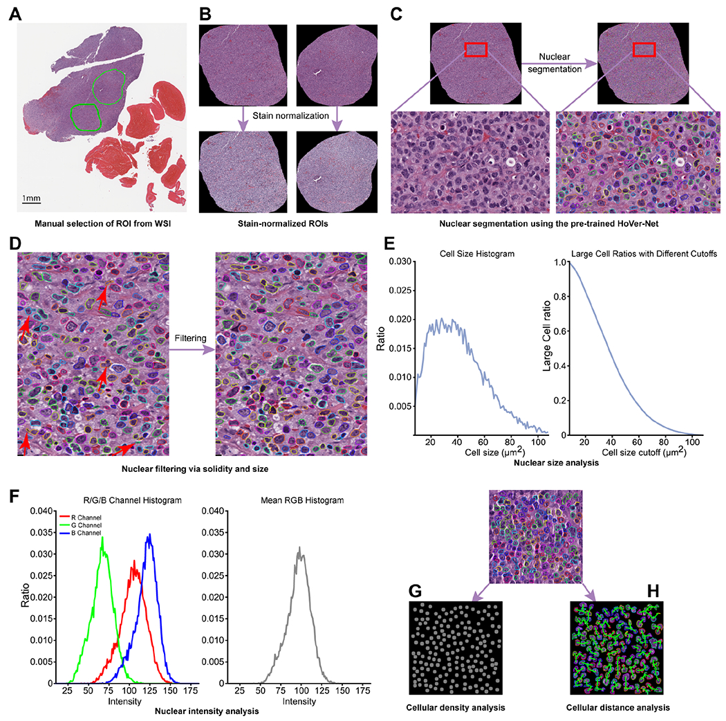
Pipeline illustrating the proposed disease diagnosis model encompassing four biomarkers (nuclear size, nuclear intensity, cellular density, and cell to nearest-neighbor distance). (A) Step 1: manual selection of ROIs from a WSI. (B) Step 2: ROI stain normalization. (C) Step 3: cell segmentation using the pre-trained Hover-Net. (D) Step 4: cell filtering is then performed via solidity and size. Steps 1 through 4 all included quality control by pathologists as needed. (E) Nuclear size analysis of the selected ROI was subsequently performed, followed by analysis of (F) nuclear intensity, (G) cellular density, and (H) nearest-neighbor distance (cellular distance for simplicity) to further enhance the performance of the disease diagnosis model. ROIs, regions of interest. WSI, whole-slide image.

Patient groups and histology slides

The study was approved by The University of Texas MD Anderson Cancer Center (UTMDACC) Institutional Review Board and conducted in accord with the Declaration of Helsinki. We retrospectively searched records for patients with hematolymphoid diseases clinically evaluated at UTMDACC between 1 February 2009 and 31 July 2021. In total, 125 patient biopsy specimens were eligible, consisting of 69 CLL slides (from 44 patients), 44 aCLL slides (from 34 patients), and 80 RT-DLBCL slides (from 47 patients). Inclusion in this study was based on the following criteria: (1) availability of archived glass slides and digital slides; (2) lymph node biopsy confirmed diagnosis; (3) availability of clinical and laboratory data to support the diagnosis in the electronic medical records. Microscopic diagnosis was confirmed in all cases by two hematopathologists (JDK and SEH), and challenging cases were resolved by a third hematopathologist (LJM). CLL and RT were defined as described by the World Health Organization Classification [15], and aCLL was defined as described previously [14]. A sizable subset (45.5%) of histology slides represented referred material from other institutions, increasing the diversity of slide sources.

Glass slides of sections stained with hematoxylin and eosin (H&E) were scanned using an Aperio AT2 scanner (Leica Biosystems, Brighton, NY, USA) at ×20 (0.50 μm/pixel). Scanning was performed in three batches within the same day, using the same scanner. The overall study group was divided equally into separate training and testing cohorts. To mitigate random effects and ensure balanced splitting, we stratified patients by matching age (above or below 60 years), gender, overall survival (>40 or <40 months for CLL, >19 or <19 months for aCLL, >9 or <9 months for RT), case source (in house versus referred consultation cases), and biopsy techniques (core-needle versus excisional). Details of patient demographic features and slide characteristics as well as the splitting of training and testing sets are outlined in Table 1.

Table 1.

Training and testing sets based on patients’ age, gender, overall survival, case source, and biopsy technique.

	Training										Testing
	Age*		Gender		Case source		Biopsy technique				Age		Gender		Case source		Biopsy technique
	>60	<60	M	F	I	O	E	CNB	OS		>60	<60	M	F	I	O	E	CNB	OS
					NCLL = 22										NCLL = 22
CLL									>40	<40									>40	<40
	9	13	15	7	11	11	11	11	9	13	9	13	14	8	6	16	12	9	9	13
					NaCLL = 17										NaCLL = 17
aCLL									>19	<19									>19	<19
	10	7	11	6	9	8	7	10	7	10	7	10	13	4	8	9	7	10	7	10
					NRT = 28										NRT = 29
RT									>9	<9									>9	<9
	15	13	17	11	19	9	8	20	12	16	15	14	18	11	20	9	10	19	13	16

^*Age: >60 years old at time of CLL diagnosis or <60 years old at time of CLL diagnosis.

CNB, core needle biopsy; E, excisional biopsy; F, female; I, in-house case; M, male; N, number of patients; O, outside institution case; OS, overall survival.

Image analysis

Selection of regions of interest (ROIs)

A regular lymph node excisional biopsy specimen digital slide (e.g. 80 000 × 50 000 pixels in level 0 of the digital slide pyramidal storage) contains more than two million cells. Analyzing a whole-slide image is computationally too expensive to implement, and the quality of some regions of the digital slide in some instances may not be suitable for diagnosis. For example, several kinds of tissue-processing artifacts including tissue folding, crush artifact, and tissue section thickness may result in a suboptimal whole-slide tissue assessment. To overcome these pre-analytic impediments, we adopted the region of interest (ROI) approach for cell morphology analysis. This approach is inherently similar to that taken routinely by pathologists when evaluating biopsy specimen materials. Diagnostically informative ROIs with the highest tissue quality were manually selected for subsequent analysis (Figure 1A). The gold standard was based on review of the whole slide. The ROIs were selected in a manner that is representative of the final diagnosis; for example, if a case was finally diagnosed as RT, the ROI was selected to include the predominant population on the whole slide, the large cells, and not the small residual CLL foci in the background.

The number of ROIs per slide averaged 2.4 and ranged from 1 to 8. The numbers of ROIs in CLL, aCLL, and RT were 159, 141, and 165, respectively. To ensure the availability of sufficient cells in each ROI, we limited the minimum width and height of all selected ROIs to 500 pixels, which corresponded to 0.25 mm. Total sizes of ROIs were overall very similar. Stain normalization was performed on all ROIs prior to further processing [16] (Figure 1B).

Nuclear segmentation

Nuclear segmentation is a prerequisite for H&E digital pathology computing workflow to carry out cellular feature analysis. We performed nuclear segmentation of selected ROIs using the robust and highly generalized Hover-Net [17] (Figure 1C). We avoided time-consuming cell annotation and fine-tuning processes by directly applying the Hover-Net model, which is pre-trained on the PanNuke dataset. The PanNuke dataset covers exhaustive nuclear labels across 19 different tissue types with H&E staining from The Cancer Genome Atlas (TCGA) [18]. The diversity of tissue types in the PanNuke dataset enables adequate generalization of the pre-trained Hover-Net model. The nuclear segmentation results were visually checked by a hematopathologist (SEH) to confirm their quality.

Nuclear filtering

The Hover-Net leverages the encoded information within the vertical and horizontal directions to tackle cell-clustering issues and thus provides high nuclear segmentation performance. Yet overlapping nuclei still pose substantial challenges to nuclear segmentation, as many nuclei appear to merge together (Figure 2A) and affect the sensitivity of nuclear size analysis. To overcome this challenge, we used the solidity feature to filter out segmented cells with overlapping nuclei by considering the concave contour shape of two overlapping nuclei (Figure 1D). The solidity value is defined as the ratio of segmented nuclear contour area to its convex hull area. Figure 2B shows the solidity calculation technique and illustrates nuclear segmentation samples. We only kept segmented nuclei with a solidity value larger than 0.84. By applying this threshold, at least 98% of nuclei were retained, while overlapping nuclei were largely removed. In addition, we focused our attention on segmented nuclei with pixel values between 32 and 432, corresponding to 8 μm² and 108 μm², as this approach represents a known biologic nuclear size range on histologic slides.

Figure 2.

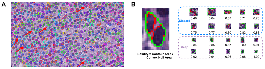
Nuclear segmentation and filtering. (A) Illustration of overlapping nuclei during nuclear segmentation step. Inaccurate segmentation (indicated by red arrows) due to overlapping nuclei appears concave in shape and results in the false impression of large cell nuclei, hindering the sensitivity of cell size analysis. (B) Nuclear filtering contour solidity measurement. Nuclear solidity is the ratio between the area of nuclear segmentation contour (red) and its convex hull area (green). Nuclei with solidity values less than 0.84 are discarded from downstream analysis.

We performed a quantitative evaluation for the Hover-Net segmented cells on 15 manually annotated patches of size 256 × 256, including five CLL, five aCLL, and five RT. Since we had a cell filtering process, we evaluated the Dice score (a commonly used to tool for evaluation of cell segmentation via AI-based algorithms) for those remaining cells after the filtering process. For each individual segmented cell, we found its corresponding cell from manual annotations and calculated the Dice score. The mean Dice scores of CLL, aCLL, and RT were 0.824, 0.835, and 0.817, respectively. The overall mean Dice score was 0.825 in the 15 total evaluated cases. The Dice scores that Hover-Net reported on the Kumar, CoNSeP, and CPM-17 datasets are 0.826, 0.853, and 0.869, respectively [19,20]. Cell segmentation performance on our dataset is compatible to Hover-Net’s reported performance, demonstrating the generalization capacity of pre-trained Hover-Net on the PanNuke dataset. We believe that cell segmentation with a Dice score over 0.8 is sufficient for downstream cellular feature extraction. Consequently, after acquiring a reasonable nuclear segmentation result for each ROI, we set the stage for nuclear size analysis.

Nuclear size

Neoplastic cells in CLL characteristically have scant cytoplasm, and thus cell size is mainly the reflection of nuclear size. Neoplastic cells in RT, on the other hand, have more cytoplasm in comparison to CLL but retain a high nuclear to cytoplasmic ratio, rendering cell size the reflection of mainly nuclear size, similar to CLL. The cellular features in cases of aCLL fall between morphologic attributes of CLL and RT. Using this rationale, for each ROI, we generated a nuclear size histogram based on nuclear segmentation results (Figure 1E). By setting a large size cutoff, nuclei were partitioned into two categories: small and large. The large nuclear ratio, defined as the number of large nuclei over the total number of nuclei, was computed for each cutoff. We first sought to identify the optimal cutoff value to best separate the three groups (CLL, aCLL, and RT). We assigned the average large nuclear ratios of CLL, aCLL, and RT as R_CLL, R_aCLL, and R_RT, and then defined (R_RT–R_aCLL)*(R_aCLL–R_CLL)*(R_RT–R_CLL) as the objective function to find the best cutoff value. By maximizing the objective function on training ROIs, we discovered that the value 24 μm was the optimal nuclear size cutoff that best distinguished CLL from aCLL and RT.

Nuclear intensity

To determine nuclear intensity defined by nuclear color composition, we obtained individual nuclear images by overlapping nuclear segmentation analysis and corresponding ROI images. The cellular intensity of CLL cells is mainly a reflection of nuclear intensity. Neoplastic cells in RT, on the other hand, although they have a moderate amount of cytoplasm in comparison to CLL, demonstrate a high nuclear to cytoplasmic ratio also rendering cellular intensity the reflection of mainly nuclear intensity. Cellular features of aCLL cells fall in between CLL and RT morphologic attributes. Using this rationale for each nucleus, we first measured the mean intensity of its R (red), G (green), and B (blue) channels. We then computed the histograms of R, G, and B intensities for each ROI; calculated the mean R, G, and B intensities; and obtained an overall mean RGB intensity for each ROI (Figure 1F).

Cellular density

Besides individual nuclear properties (e.g. size and intensity), we explored cellular density (number of cells per ROI) as a potential additional biomarker to refine diagnostic accuracy (Figure 1G). For each ROI, we counted the number of cells after nuclear segmentation and filtering, and we assigned the cell number to N_cell. In addition, we obtained the physical size of each ROI, S_roi, by counting the pixels it contains and multiplying the number of pixels by slide digitization magnification (0.50 μm/pixel). We defined the cellular density as N_cell/S_roi.

Cell to nearest-neighbor distance

We then sought to investigate the distance between neighboring cells (Figure 1H). For each cell inside a given ROI, we measured its Euclidean distances to other cells via their spatial coordinates. We identified the cell with the smallest Euclidean distance as the nearest neighbor, and its distance to the cell of interest was considered as the cell to nearest-neighbor distance. We then calculated the mean value of all cell to nearest-neighbor distances in a given ROI.

Disease diagnosis model

Based on the above cellular and architectural biomarkers (nuclear size, nuclear intensity, cellular density, and cellular distance), we conducted two diagnostic experiments on annotated ROIs from the three groups. In the first experiment, we trained the disease diagnosis model using the training patient cohort and evaluated the performance of the model using the testing patient cohort. Details about the training and testing cohorts are outlined in Table 1.

We aimed to balance the training and validation datasets by controlling variables such as age, gender, case source, biopsy techniques, and overall survival (Table 1). In the second diagnostic experiment, we performed repeated splitting analysis in which we combined the training and testing cohorts and then randomly split them into training and testing sets based on patients with a ratio of 1:1, for 100 times. Patient-based splitting was performed to avoid running into ROIs belonging to the same patients in both the training and testing sets, which may lead to information leakage. We then reported the mean and standard deviation of disease diagnosis on the 100 times splitting-basis to avoid any potential biases that might be caused by one-time splitting, and we further validated our model’s generalizability and robustness. The repeated splitting test was aimed at strengthening the statistical significance of the analysis. In fact, when conducting a t-test, a sample size of n ≥ 30 is treated as large based on the statistical theory. We chose to repeat splitting 100 times in our model as a balance between sample size and computational cost. We conducted experiments to explore the effects of repeated splitting times: We experimented with repeated splitting times ranging from 60 to 200 and found that the diagnostic performance was quite consistent among different numbers within this range (data not shown). For both diagnostic experiments, we used the Random Forest classifier from the Python scikit-learn package (version 0.24).

Statistical analyses

Biomarker statistical significance analysis of our diagnostic model was calculated by applying Welch’s t-test, using the Python SciPy package (version 1.6.1). The receiver operating characteristics (ROC) curve analysis and area under the curve (AUC) were used to assess the prediction capability of the proposed imaging models.

Results

Individual biomarker analysis

Nuclear size

For each ROI, we drew a nuclear size histogram and calculated the mean and standard deviation of the histograms for CLL, aCLL, and RT (Figure 3A). Nuclei in CLL ROIs clustered around 20 μm². In aCLL cases, ROIs had a mean size close to 20 μm² but a sizeable portion of ROIs harbored cells with a larger nuclear size, resulting in a more widely spread nuclear size histogram in comparison with CLL cases. In contrast, RT ROIs harbored a higher number of cells with nuclear size larger than 20 μm², resulting in a mean histogram extruding on regions with nuclear size larger than 20 μm².

Figure 3.

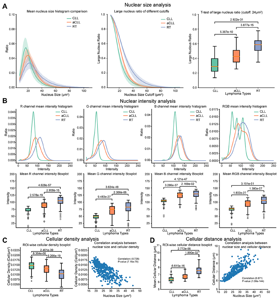
Nuclear size and intensity, and cellular density and distance analyses. (A) Nuclear size analysis performed on CLL, aCLL, and RT ROIs. The mean nuclear size histogram across ROIs is plotted, with a differential distribution among the three entities in question. Large nuclear ratio of different cutoffs is analyzed to identify the optimal cutoff to best separate the three entities. A t-test of large nuclear ratio, using a cutoff of 24 μm, demonstrates statistically significant differences among CLL, aCLL, and RT ROIs. (B) Nuclear intensity analysis performed on CLL, aCLL, and RT ROIs. Illustration of the mean nuclear intensity in the red, green, and blue channels plotted separately and then combined with a differential distribution among CLL, on the one hand, and aCLL/RT, on the other hand. Analysis of the mean nuclear intensity in the three separate channels, then in combination, demonstrates a statistically relevant difference among CLL, aCLL, and RT. (C) Cellular density analysis performed on CLL, aCLL, and RT ROIs. The mean cellular density is plotted, with a significant statistical difference among the three entities in question. A negative correlation (−0.728) is demonstrated between nuclear size and cellular density, with a statistically significant P value. (D) Cell to nearest-neighbor distance analysis performed on CLL, aCLL, and RT ROIs. The mean of cell to nearest-neighbor distance (cellular distance for simplicity) is plotted, with a significant statistical difference among the three entities in question. A positive correlation (0.871) is demonstrated between cell size and cell to nearest-neighbor distance analysis, with a statistically significant P value. ROIs, regions of interest; CLL, CLL/SLL; aCLL, accelerated CLL; RT, Richter transformation-large B-cell lymphoma variant; RGB, red green blue.

We plotted the large nuclear ratios of ROIs belonging to CLL, aCLL, and RT with varying cutoffs, as shown in Figure 3A. On a wide range of cutoff values, CLL and aCLL ROIs were found to have closer large nuclear ratios, whereas RT ROIs demonstrated larger nuclear ratios in comparison to CLL and aCLL. Using the proposed objective function (R_RT–R_aCLL)*(R_aCLL–R_CLL)*(R_RT–R_CLL), we found that the cutoff value 24 μm² yielded the best separation among the three groups on training data. Based on this cutoff, we computed the large nuclear ratio for each ROI, as illustrated in the boxplot of Figure 3A. The large nuclear ratios exhibited a crescendo trend from CLL to aCLL and into RT with a statistically significant difference (p < 0.05). However, based on this biomarker alone, there was still considerable overlap between CLL and aCLL, as well as aCLL and RT. To enhance the separation among the three groups, we sequentially added three more biomarkers, as detailed below.

Nuclear intensity

We plotted the mean nuclear intensity histogram for the CLL, aCLL, and RT ROIs using the R, G, B, and mean RGB channels as illustrated in Figure 3B. The aCLL and RT ROIs showed higher mean values in different channels, whereas nuclei in the CLL ROIs demonstrated the smallest values overall. We then plotted the mean ROI nuclear intensity across the four different channels for the three groups, as illustrated in Figure 3B. CLL ROIs had smaller mean levels across all channels compared with aCLL and RT (p < 0.05). There were also significant differences between the mean ROI levels between aCLL and RT cases (p < 0.05), but the differences between aCLL and RT were less prominent compared with the differences between CLL and aCLL, as both mean ROI levels in the B channel centered around the same value (~130) (Figure 3B).

Cellular density

Nuclear size and intensity are features used by hematopathologists to evaluate disease progression. Assessment of cellular density (i.e. number of cells occupying a given space) is another diagnostic dimension exploited during manual diagnostic evaluation in clinical practice. To enhance diagnostic performance, we sought to explore this feature by calculating cellular density defined as cell aggregates per square micrometer within an ROI. In Figure 3C, we plotted cellular densities in CLL, aCLL, and RT ROIs. We observed that the mean cellular density decreases significantly from CLL to RT ROIs. Although CLL and aCLL ROIs demonstrated closer cell density values compared with RT, all three pairs (CLL/aCLL, aCLL/RT, CLL/RT) showed significant cellular density differences (p < 0.05). We posited that the cellular density results in a given square micrometer of RT ROI occupied by a smaller number of large cells, versus a larger number of smaller cells in CLL or aCLL ROIs. To explore this point, we plotted the ROI mean cell size and cell density values in Figure 3C and indeed found a negative correlation between cell size and cell density (Pearson correlation coefficient = −0.728, p = 7.16e-78).

Cell to nearest-neighbor distance

Unlike most other parameters, cellular spatial relationships are not intuitively or easily applied by hematopathologists during manual morphologic evaluation. In view of the key implications that cellular composition and the tumor microenvironment have in the context of CLL disease evolution, we contended that extracting such data through a deep learning algorithm would add power to our diagnostic model. To explore the spatial relationships among cells, we investigated the cell to nearest-neighbor cell distance in CLL, aCLL, and RT ROIs, and plotted their mean values (Figure 3D). RT ROIs showed the largest cell to nearest-neighbor distance among the three groups, whereas mean cellular distance is somewhat closer in aCLL and CLL ROIs; a significant difference (p < 0.05) exists among the three disease groups.

We posited for this parameter that a given square micrometer of RT ROI is occupied by a smaller number of large cells with resultant larger cellular distances, versus a larger number of smaller CLL and aCLL cells with smaller cellular distances in CLL or aCLL ROIs. To explore this point, we plotted the mean cell size and cell distance in Figure 3D and indeed found a positive correlation between these two parameters (Pearson correlation coefficient = 0.871, p = 1.08e-144).

Performance of the disease diagnosis model

Based on univariate testing, the descending order of diagnostic predictive values of the biomarkers was as follows: nuclear size (0.657) > cellular distance (0.640) > nuclear intensity (0.586) > cellular density (0.566) and nuclear intensity (0.821) > cellular distance (0.810) > nuclear size (0.797) > cellular density (0.748), for accuracy and area under the curve (AUC), respectively (Figure 4A–D). To overcome overlapping morphologic attributes in the disease groups and enhance diagnostic accuracy, we sought to combine sequentially the above-described biomarkers as shown in the confusion matrix illustrated in Figure 4E–G. We started first by adding nuclear size and intensity since these two features are intuitively sought after in hematopathology practice, and both nuclear size and intensity demonstrated the highest accuracy and AUC among other biomarkers, respectively (Figure 4E), followed by the addition of cellular density (Figure 4F) and, lastly, cellular distance (Figure 4G). By adding more biomarkers, we were able to increase the overall diagnostic performance, as shown in the accuracy and AUC metrics. Namely, accuracy and AUC increased from 0.657 and 0.797, respectively, based solely on cell size to 0.824 and 0.935, respectively, after nuclear intensity, cell density, and cell distance were added.

Figure 4.

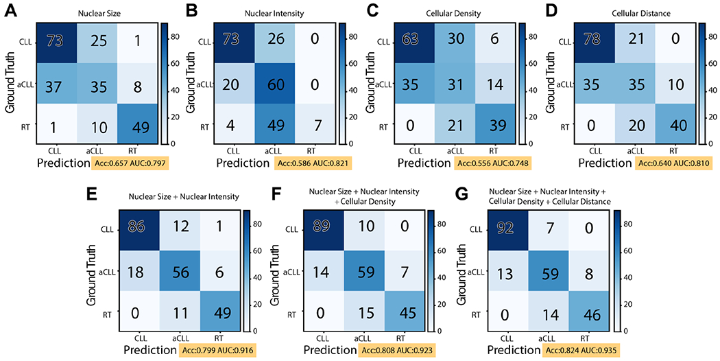
Confusion matrix illustrating the predictive ability of the disease diagnosis model on the testing set. (A–D) Univariate biomarker predictive values based on nuclear size, nuclear intensity, cellular density, and cell to nearest-neighbor distance (cellular distance for simplicity). (E) By adding nuclear intensity and nuclear size, the diagnostic accuracy is increased from 0.657 to 0.799. (F) Further addition of cellular density increased the diagnostic accuracy to 0.808. (G) Combining all four identified biomarkers, including cell to nearest-neighbor distance, resulted in an accuracy of 0.824 and an AUC of 0.935 of the disease diagnosis model.

Repeated splitting analysis

The above-described experiments were conducted in a single splitting round (one training and one testing set), which may not fully transmit the general applicability and stability of our diagnostic model. To validate the stability and robustness of the four identified biomarkers, we combined all ROIs together and randomly split them into training and testing sets for 100 times based on patient identification, and then evaluated diagnostic performance. The performance of the repeated splitting analysis is illustrated in Figure 5. Similar to single training/testing splitting, a gradual performance enhancement is observed as more biomarkers are added, with a gradual increase in both the accuracy and the AUC metrics. The statistical significance of both accuracy and AUC is enhanced as new biomarkers are added. When gradually adding three biomarkers, the P values for accuracy are 1.815e-41, 1.202e-12, and 0.015; and the P values for AUC are 9.064e-45, 7.045e-35, and 6.020e-05, respectively. Furthermore, comparison of the mean accuracy and AUC of the repeated splitting analysis with the accuracy and AUC from the first single training/test splitting shows that their values are close to each other when the same number of biomarkers is used.

Figure 5.

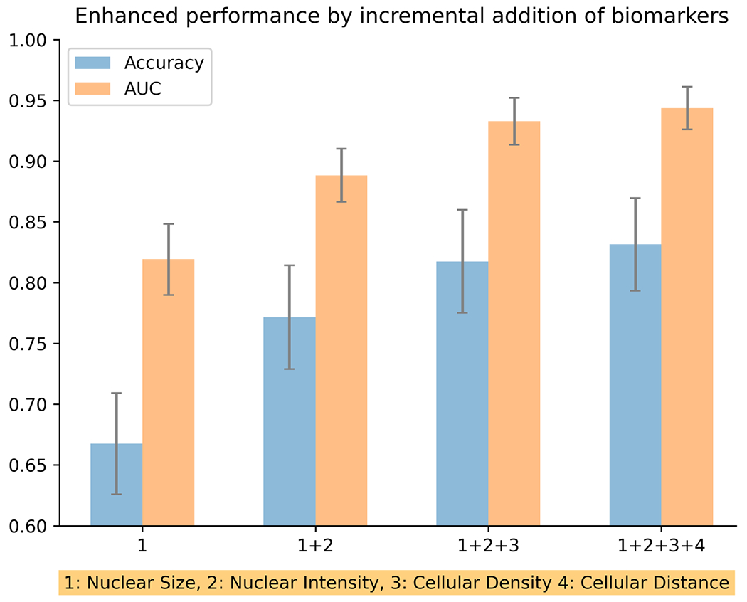
Repeated splitting analysis with incremental addition of disease diagnosis biomarkers. By performing train/test splitting for 100 times, and following the gradual addition of biomarkers, a very robust gradual increase in mean disease diagnosis accuracy and mean area under the curve (AUC) is observed.

Discussion

The use of deep learning algorithms to enhance diagnostic morphologic evaluation has been gaining popularity at an unprecedented pace. However, such advances have been limited in the field of lymphoid neoplasia, where diagnostic evaluation is typically complex, as it relies on a broad constellation of morphologic attributes. In B-cell lymphomas, such attributes could be inherent to the neoplastic cells themselves and their ability to differentiate along a variety of pathways and, equally importantly, to the cellular and stromal components within the tumor microenvironment. These attributes are at play in biopsy samples from patients with CLL, whose evaluation could occur within a variety of clinical contexts ranging from baseline incidental discovery of the disease to a suspicion of acceleration or transformation at any point during the course of the disease, often prompted by laboratory studies and/or exacerbation of systemic symptoms. Thus, while a diagnosis of CLL is usually straightforward, various factors contribute to making the diagnosis of aCLL and RT challenging, particularly in scant targeted needle core biopsy specimens in which the morphologic and architectural features may not be fully representative of the underlying disease [13]. Our design was inspired by clinical challenges encountered in clinical practice. In order to navigate and overcome inevitable diagnostic obstacles and impediments dictated by limited tissue samples and pre-analytical variables, we sought to conceptualize an AI-based disease diagnosis model to objectively assist in the evaluation of tissue samples from CLL patients with clinical suspicion of disease progression. This clinically oriented model is amenable to further optimization, validation, and possible implementation into pathology clinical practice as the technology driving digital pathology unfolds and becomes more widely available. Adopting such AI-based models into clinical practice is predicted to improve diagnostic accuracy and reproducibility, and possibly identify biologic attributes and prognostic parameters.

The first building blocks of our diagnostic model included nuclear size and nuclear intensity, two features intuitively used by pathologists in clinical practice to evaluate CLL. The number of larger nuclei is directly proportional to the extent of disease progression, and increased nuclear intensity is reflective of open and vesicular nuclear chromatin indicating increased nuclear activity, and translates into an increased cellular metabolism and proliferation rate. However, using these two aforementioned methods alone left persistent overlap across a number of CLL and aCLL ROIs. This overlap could be explained by the fact that aCLL is likely a mid-point in the spectrum of biologic progression of CLL, with more aggressive features that are not necessarily limited to nuclear size and intensity but rather characterized by increased mitotic activity and expanded proliferation centers, among other features. In addition, a number of RT-DLBCL ROIs bled into the CLL cell size zone. This finding is likely explained by disease-specific biologic factors (e.g. stromal fibrosis frequently occurs in RT) and technical factors, including crush artifact and suboptimal tissue processing (e.g. thick tissue sections in RT result in decreased intensity). These biologic and pre-analytical impediments prompted us to experiment with unconventional features such as cellular density and cell to nearest-neighbor distance, in order to improve our disease diagnosis model.

We observed that a given CLL ROI is populated by a large number of cells with small-sized nuclei, with decreased intercellular distance. In contrast, a given RT ROI is populated by a smaller number of cells with large-sized nuclei, with increased intercellular distance. By exploiting the cellular density and cell to nearest-neighbor distance, we enhanced the accuracy of our diagnostic model from 0.799 (based on combined cell size and intensity) to 0.808 and 0.824, based on the addition of cellular density and cell to nearest-neighbor distance, respectively. Limitations to cell to nearest-neighbor distance analysis included, but were not restricted to, tissue fixation artifact and treatment induced fibrosis, necrosis, and hemorrhage, creating an artifactual increase in cell distance. Based on the results from the confusion matrix, aCLL remained the most challenging entity to fully characterize. However, an undeniable gradual improvement was observed as more biomarkers were added. In addition, our disease diagnosis model showed a remarkable performance in diagnosing CLL and RT-DLBCL, with minor overlaps of these two categories with aCLL, following the addition and analysis of all four biomarkers.

In contrast to other studies evaluating AI for the diagnosis of lymphoid neoplasms [7–10,12], we harnessed the power of deep learning to automate the key histologic features based on hematopathology field knowledge rather than adopting a ‘black-box’ scheme. Of note, our model with four clinically meaningful features has achieved an AUC of 0.935. A general challenge for deep learning models is their generalizability, rooted from model overfitting. In other words, these black-box models usually have a significant drop when testing on unseen datasets. By contrast, we expect our model to be more robust because it contains only four features to mitigate overfitting risk from a statistical perspective. Further, since these features are distilled from clinical practice, we anticipate that this model, with appropriate validation, is more likely to be translated into clinical practice. Beyond tissue H&E slides, we envision that our proposed analysis can also be transitioned into blood cell image analysis. Currently, three main classes of quantitative features are proposed to optimize morphology through blood cell digital image processing techniques to aid in the diagnosis of lymphomas (see review elsewhere [21]), including geometrics, color, and texture.

There are several limitations to this study. Although our model performed robustly with 45.5% of analyzed histology slides being referred from other institutions, it warrants further validation in a prospective multicenter setting. This hybrid design integrates deep learning with pre-existing human knowledge from pathologists applied through manually annotated ROIs. Such annotation excludes artifacts and residual areas of clear CLL in cases of RT and aCLL, for example. We will be striving to develop an automated ROI selection algorithm in future iterations of our model. In addition, the analysis of cellular interactions based on cellular density and cellular distance is rudimentary and may not be able to characterize the complex spatial patterns of the tumor microenvironment. This limitation might explain why adding these two features improved the model only marginally. To improve this model, we will need to craft more sophisticated features and analytics to better profile spatial interaction patterns in the future.

In summary, our disease diagnosis model validates the assumption that designing new biomarkers based on morphologic, architectural, and microenvironmental features can boost the diagnostic accuracy of disease entities or stages of progression within a single disease entity, as illustrated in this study assessing CLL, aCLL, and RT. The results of this study also highlight the importance of identifying more biomarkers in the future to enhance disease diagnosis performance in challenging clinical scenarios.

References

- 1.Coudray N, Ocampo PS, Sakellaropoulos T, et al. Classification and mutation prediction from non-small cell lung cancer histopathology images using deep learning. Nat Med 2018; 24: 1559–1567. [DOI] [PMC free article] [PubMed] [Google Scholar]
- 2.Kather JN, Pearson AT, Halama N, et al. Deep learning can predict microsatellite instability directly from histology in gastrointestinal cancer. Nat Med 2019; 25: 1054–1056. [DOI] [PMC free article] [PubMed] [Google Scholar]
- 3.Campanella G, Hanna MG, Geneslaw L, et al. Clinical-grade computational pathology using weakly supervised deep learning on whole slide images. Nat Med 2019; 25: 1301–1309. [DOI] [PMC free article] [PubMed] [Google Scholar]
- 4.Courtiol P, Maussion C, Moarii M, et al. Deep learning-based classification of mesothelioma improves prediction of patient outcome. Nat Med 2019; 25: 1519–1525. [DOI] [PubMed] [Google Scholar]
- 5.Chen P, Gao L, Shi X, et al. Fully automatic knee osteoarthritis severity grading using deep neural networks with a novel ordinal loss. Comput Med Imaging Graph 2019; 75: 84–92. [DOI] [PMC free article] [PubMed] [Google Scholar]
- 6.Syrykh C, Abreu A, Amara N, et al. Accurate diagnosis of lymphoma on whole-slide histopathology images using deep learning. NPJ Digit Med 2020; 3: 63. [DOI] [PMC free article] [PubMed] [Google Scholar]
- 7.Li D, Bledsoe JR, Zeng Y, et al. A deep learning diagnostic platform for diffuse large B-cell lymphoma with high accuracy across multiple hospitals. Nat Commun 2020; 11: 6004. [DOI] [PMC free article] [PubMed] [Google Scholar]
- 8.Miyoshi H, Sato K, Kabeya Y, et al. Deep learning shows the capability of high-level computer-aided diagnosis in malignant lymphoma. Lab Invest 2020; 100: 1300–1310. [DOI] [PubMed] [Google Scholar]
- 9.Achi HE, Belousova T, Chen L, et al. Automated diagnosis of lymphoma with digital pathology images using deep learning. Ann Clin Lab Sci 2019; 49: 153–160. [PubMed] [Google Scholar]
- 10.Mohlman JS, Leventhal SD, Hansen T, et al. Improving augmented human intelligence to distinguish Burkitt lymphoma from diffuse large B-cell lymphoma cases. Am J Clin Pathol 2020; 153: 743–759. [DOI] [PubMed] [Google Scholar]
- 11.El Achi H, Khoury JD. Artificial intelligence and digital microscopy applications in diagnostic hematopathology. Cancers (Basel) 2020; 12: 797. [DOI] [PMC free article] [PubMed] [Google Scholar]
- 12.Irshaid L, Bleiberg J, Weinberger E, et al. Histopathologic and machine deep learning criteria to predict lymphoma transformation in bone marrow biopsies. Arch Pathol Lab Med 2021. 10.5858/arpa.2020-0510-OA. [DOI] [PubMed] [Google Scholar]
- 13.Agbay RL, Jain N, Loghavi S, et al. Histologic transformation of chronic lymphocytic leukemia/small lymphocytic lymphoma. Am J Hematol 2016; 91: 1036–1043. [DOI] [PubMed] [Google Scholar]
- 14.Giné E, Martinez A, Villamor N, et al. Expanded and highly active proliferation centers identify a histological subtype of chronic lymphocytic leukemia (“accelerated” chronic lymphocytic leukemia) with aggressive clinical behavior. Haematologica 2010; 95: 1526–1533. [DOI] [PMC free article] [PubMed] [Google Scholar]
- 15.Swerdlow SH, Campo E, Harris NL, et al. Chronic lymphocytic leukaemia/small lymphocytic lymphoma. In WHO Classification of Tumours of Haematopoietic and Lymphoid Tissues (Revised 4th edn). IARC: Lyon, 2017; 216–221. [Google Scholar]
- 16.Reinhard E, Adhikhmin M, Gooch B, et al. Color transfer between images. IEEE Computer Graphics and Applications 2001; 21: 34–41. [Google Scholar]
- 17.Graham S, Vu Q, Raza SEA, et al. Hover-Net: simultaneous segmentation and classification of nuclei in multi-tissue histology images. Med Image Anal 2019; 58: 101563. [DOI] [PubMed] [Google Scholar]
- 18.Gamper J, Alemi Koohbanani N, Benet K, et al. PanNuke: an open pan-cancer histology dataset for nuclei instance segmentation and classification. In Digital Pathology. ECDP 2019. Lecture Notes in Computer Science (Vol. 11435), Reyes-Aldasoro C, Janowczyk A, Veta M, et al. (eds). Springer: Cham, 2019. 10.1007/978-3-030-23937-4_2. [DOI] [Google Scholar]
- 19.Kumar N, Verma R, Sharma S, et al. A dataset and a technique for generalized nuclear segmentation for computational pathology. IEEE Trans Med Imaging 2017; 36: 1550–1560. [DOI] [PubMed] [Google Scholar]
- 20.Vu QD, Graham S, Kurc T, et al. Methods for segmentation and classification of digital microscopy tissue images. Front Bioeng Biotechnol 2019; 7: 53. [DOI] [PMC free article] [PubMed] [Google Scholar]
- 21.Merino A, Puigví L, Boldú L, et al. Optimizing morphology through blood cell image analysis. Int J Lab Hematol 2018; 40(suppl 1): 54–61. [DOI] [PubMed] [Google Scholar]