A mathematical model of the within-host kinetics of SARS-CoV-2 neutralizing antibodies following COVID-19 vaccination

Abstract

Compelling evidence continues to build to support the idea that SARS-CoV-2 Neutralizing Antibody (NAb) levels in an individual can serve as an important indicator of the strength of protective immunity against infection. It is not well understood why NAb levels in some individuals remain high over time, while in others levels decline rapidly. In this work, we present a two-state mathematical model of within-host NAb dynamics in response to vaccination. By fitting only four host-specific parameters, the model is able to capture individual-specific NAb levels over time as measured by the AditxtScore™ for NAbs. The model can serve as a foundation for predicting NAb levels in the long-term, understanding connections between NAb levels, protective immunity, and breakthrough infections, and potentially guiding decisions about whether and when a booster vaccination may be warranted.

Graphical abstract

1. Introduction

SARS-CoV-2 Neutralizing Antibody (NAb) levels in an individual have been shown to be correlated to the strength of protective immunity against infection (Khoury et al., 2021, Krammer, 2021, Addetia et al., 2020, Dispinseri et al., 2021). Antibodies develop both in response to infection and to vaccination. Both non-neutralizing and neutralizing antibodies are involved in the immune response to viral infection, serving to alert effector cells to the presence of pathogen in infected cells as well as to disrupt the ability of a virus to enter a host cell. As pointed out in Murin et al. (2019), neutralizing antibodies that develop under viral load pressures serve as sentinels that provide insight into the associated humoral response.

The focus of the model in our study is on understanding changes in individual-specific NAb concentrations in fully vaccinated individuals using a novel flow-cytometry-based NAb assay. NAb activity levels can be measured using two general approaches: Bioassays, which determine the ability of NAb to prevent viral infection of cells in culture media, and binding assays, which evaluate the ability of NAb to prevent binding of SARS-CoV-2 spike protein to the ACE-2 receptor on the surface of human cells. While the former is the gold standard for determining the effectiveness of antibodies to neutralize viral entry into cells, bioassays require more time and higher safety level laboratories and are, therefore, more expensive. Binding assays can serve as a more practical and scalable methodology to assess NAb levels. The novel flow-cytometry test that was used in this study was compared to a bioassay (Vandergaast et al., 2021) to determine its performance using samples from 40 positive and negative samples in a blinded study. Results showed 100% concordance between the two methodologies in quantifying NAb levels in the samples (unpublished data).

Our interest is in whether an individual is protected from getting infected, which is directly connected to the action of the NAbs. Over time, NAb levels in some individuals remain high, while in others levels decline rapidly. Since NAb levels are promising as indicators of the protective potential of the immune response to a viral challenge, our goal is to develop a mathematical model that can serve as a starting point for improving our ability to predict an individual’s NAb response to mRNA vaccine dosing, persistence of immune strength, and how quickly immunity levels may wane.

Note that the question we are asking is not about how severe the illness will be in an infected individual. To address that question, we would also consider the cellular immune response. In our case, however, it is clear that if we do not have upstream T-cell recognition, we will not have formation of memory or B cell activation, and subsequently we will not have plasma cells or antibody production. For the purpose of addressing the question of protection against infection, using neutralizing antibodies in the context of the two mRNA vaccines studied to evaluate the durability of neutralization and likely degree of immune protection against infection within an individual is an approach that is both simple (with relatively few model parameters required) and can provide insight. The data used in our study are all from COVID-19-naive individuals. We recognize that in individuals who have had a convalescence history there will be more involved in the immune response to vaccination than just response to the spike protein, since through natural infection, the immune system would have been exposed to more than just the spike protein.

In this work, we present a two-population mathematical model of within-host NAb dynamics in response to vaccination. By fitting only four subject-specific parameters, model simulations can capture NAb level changes within an individual measured by the AditxtScore™ for NAbs. The model can serve a foundation for predicting NAb levels over time and guiding decisions about whether and when a booster vaccination may be warranted.

1.1. mRNA vaccines

Both of the newly developed mRNA vaccines widely available in the U.S. function differently from traditional live-attenuated or disabled virus vaccines. The SARS-CoV-2 mRNA vaccine encodes for the spike protein, which harbors the receptor binding domain (RBD), to elicit the immune response. One of the effects of the immune response is production of neutralizing antibodies (NAb) that bind to the RBD thereby preventing viral entry into the host cells. The correlation between how mRNA vaccines work and elicit production of NAb, which then interfere with binding of the spike protein to the cell receptor required for viral entry into the cell, indicates that evaluating NAb levels and NAb trajectories over time is important in understanding the likelihood of an individual having protective immunity against infection.

1.2. Mathematical models of within-host responses

Since the outbreak of SARS-CoV-2 near the end of 2019, a number of mathematical models have been created to help guide medical care providers and health policy makers in establishing approaches to stemming the spread of disease and determining best practices for treatment and prevention. While many useful models focus on modeling epidemiological dynamics and answering questions about population-level effects of interventions such as vaccination and treatment (c.f. Diagne et al., 2021, Swan et al., 2021), our interest is in addressing questions about protective immunity within a vaccinated individual. Some excellent within-host mathematical models have been developed to focus on a variety of questions about response to virus, treatment, and vaccination. Most of these models use patient data to determine population-level parameterization, that is, parameter values that are meant to reflect the within-host responses of an “average” individual. New models are continually being created, so our sample of within-host models below is by no means a comprehensive list, but is meant to provide the context that motivated us to build our model.

Li et al. (2020) have a within-host viral dynamic model of live infection with SARS-CoV-2 using chest radiograph score data to determine model parameters. The focus of the model is on simulating viral growth within the lung. With a system of ordinary differential equations, it tracks three populations: uninfected and infected pulmonary epithelial cells and viral load. The model is used to explore the effect of treatment timing and patient immune strength, and was later analyzed mathematically in Nath et al. (2021) with the aim of laying a foundation for exploring treatment interventions in silico. There are nine model parameters, seven of which are fit at a population level using data from two published studies Pan et al. (2020) and Oh et al. (2016) via Markov-Chain Monte Carlo optimizations.

Farhang-Sardroodi et al. (2021) created a within-host model of the immune response to an adenovirus-based vaccine. Using ordinary differential equations, they investigated the impact of various dosing strategies, and captured dose-dependent responses. Model parameters were fit to clinical trial data for the AstraZeneca/Oxford vaccine (Ramasamy et al., 2020). Data from a binding and neutralization study collected from COVID-19 recovered patients (Wu et al., 2020) were used to compare antibody-level predictions. The overarching aim of the Farhang–Sarhoodi investigation was to determine how best to conserve vaccine doses while providing necessary levels of protection. The model includes seven population state variables: non-replicating vaccine cell particles, helper T-cells, cytotoxic T-cells, IFN-$\gamma$, IL-$6$, plasma B-cells, and an antibody population. The antibodies in this model are stimulated by plasma B-cells which are indirectly stimulated by the presence of vaccine cell particles. The model antibodies in turn clear or neutralize vaccine cell particles. There are twenty-one model parameters, twelve of which are found by fitting the model to data to determine population-level ranges.

The goal of the model by Kim et al. (2021), which does not account for vaccination, is to use viral-load data to compare within-host dynamics of SARS-CoV2, MERS-CoV, and SARS-CoV with the aim of gaining more insight into SARS-CoV2 behaviors and improved treatment strategies. Using simplifying assumptions the model is reduced to a set of two bilinear ordinary differential equations that track levels over time of the number of coronavirus RNA copies and the fraction of infected target cells. With this simple form, the authors are able to insert treatment terms to explore hypothetical combination therapies. Patient data were fit simultaneously using a nonlinear mixed effects approach to determine model parameter values. With this model the authors determine that therapies that block virus production are likely to be effective only if initiated before the viral load peak. There are eight population-level parameter values for each of the three virus types.

The model by Sadria and Layton (2021) is built to track the interactions between SARS-CoV-2 and the immune response, and is meant to provide a testbed for simulating the effects of drug treatments against SARS-CoV-2 infection. The strength of this model is in how comprehensive it is. The authors track the control of SARS-CoV-2 infection by both the innate and adaptive immune responses. Data from viral load studies are used to determine model parameters, and three treatment options are simulated: Remdesivir, convalescent plasma, and a hypothetical therapy that inhibits virus entry into host cells. The populations tracked by the model include viral load, healthy cells, latent cells (which serve as hosts for replicating virus), infected cells, antigen presenting cells, interferon, effector cells, plasma cells, virus-specific antibodies that serve to neutralize and eliminate virus, the fraction of damaged cells, and a measure of specificity (a metric that increases as plasma cells produce antibodies that are more compatible with viral antigen). The model provides a foundation for the development of a platform for in silico testing of potential therapies and vaccines for COVID-19. There are twenty-nine population-level model parameters.

Other mathematical models of SARS-CoV-2 within-host dynamics include Ejima et al. (2020), Hernandez-Vargas and Velasco-Hernandez (2020), Kim et al. (2020), Sahoo et al. (2020), and Chatterjee et al. (2021) with each model focusing on somewhat different questions. Model parameters are fit to a variety of data sets measuring viral load, antibody levels, and certain immune response rates, and tend to be determined at a population level.

We have learned a great deal since the start of the world-wide outbreak about how SARS-CoV-2 affects individuals, but it is still not well-understood why some infected individuals experience only mild symptoms, with some even remaining asymptomatic, while for others, infection with SARS-CoV-2 can result in severe respiratory symptoms and even death. As Chatterjee et al. (2021) point out, the reasons for the extreme heterogeneity in outcomes of SARS-CoV-2 infection across individuals is still unclear, but they hypothesize that this heterogeneity arises from variations in the strength and timing of an individual’s immune response. Most within-host models provide model parameterization for immune responses to infection at a population level, but we want to move toward being able to help an individual understand how robust their own immune response is likely to be. Our aim is to provide a mathematical model that is as simple as possible (our model has only two state variables), with as few parameters as possible (only four subject-specific parameters must be fit for an individual), so that determining subject-specific parameters is a tractable task. With the model in this paper we can provide subject-specific insight regarding individual levels of likely immune protection against infection in a fully vaccinated individual using neutralizing antibody (NAb) levels as our indicator.

2. Materials and methods

2.1. Assay data

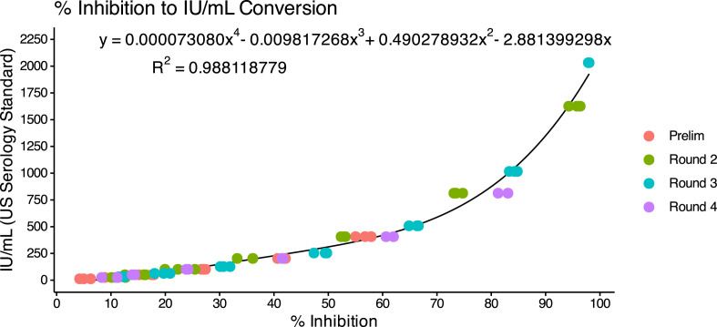
The AditxtScore™ test for neutralizing antibodies to SARS-CoV-2 is a novel flow cytometry based competitive inhibition assay for the measurement of total neutralizing antibodies to SARS-CoV-2 in human plasma samples. Microparticles coated with the recombinant SARS-CoV-2 RBD antigen are incubated with biotinylated angiotensin converting enzyme-2 (ACE-2), human subject plasma or phosphate buffered saline (PBS), and fluorescent labeled streptavidin. Neutralizing antibodies in the subject plasma sample bind to the RBD antigen and inhibit binding of ACE-2 to the RBD antigen. Following incubation, the beads are washed and then measured by flow cytometry to determine the degree of inhibition of ACE-2 binding. The degree of inhibition of the ACE-2 binding is proportional to the amount of neutralizing antibodies present in the human subject sample. Zero or near zero percent ACE-2 binding inhibition is observed when phosphate buffered saline is used as sample or when no neutralizing antibodies are present in the subject sample. Human subject plasma samples with higher concentrations of neutralizing antibodies will produce % binding inhibition values up to 100%. One hundred percent binding inhibition is achieved when ACE-2 is completely inhibited from binding to the RBD coated microparticles by the neutralizing antibodies in the sample. Sample % ACE-2 binding inhibition values are compared to a standard curve with known neutralizing antibody values in International Units per milliliter (IU/mL) to convert percent inhibition values into units of IU/mL for each subject sample tested. A standard curve was generated using dilutions of the human NIH SARS-CoV-2 serology standard, Lot $\#$ COVID-NS01097, characterized and made available by Frederick National Laboratory for Cancer Research (FNLCR), Frederick, Maryland, USA. The FNLCR standard has been assigned Potency for Functional Activity (Neutralizing Unitage) of 813 IU/mL as calibrated to the primary standard WHO SARS-CoV-2 Serology Standard. A dilution series of standard was prepared with standard concentrations accounting for values of 2032.5, 1626, 1016, 813, 406.5, 203.2, 101.6, 50.8, and 25.4 IU/mL. IU/mL values were plotted against neutralizing antibody $\text{\%}$ inhibition values measured by flow cytometry for each standard dilution. The resulting standard curve was fit using a polynomial curve fit function and the curve equation was used to generate IU/mL values from $\text{\%}$ inhibition values for all samples measured. Fig. 1 shows the calibration curve derived over four days of runs and the resulting polynomial equation.

Fig. 1.

Calibration curve for converting % inhibition to IU/mL. Resulting polynomial fit: $y=(7.3\times 10^{-5})x^4-(9.8\times 10^{-3})x^3+(4.9\times 10^{-1})x^2-2.9x$.

Precision of the method was determined using 4 subjects with 4 different IU/mL values, 6 assays per day for 3 days. Precision varied somewhat among subjects (details are included in Appendix B). The coefficient of variation (%CV) was inversely proportional to IU/mL, thus precision is higher for higher NAb levels in IU/mL. For our visualizations of the data, we used a coarse-grained assignment of precision results for four concentration ranges. Values are shown in Table 1.

Table 1.

Coarse-grained precision of method to determine AditxtScore™ for neutralizing antibodies (NAb) to SARS-CoV-2, given in four IU/mL interval ranges. Precision as measured by coefficient of variation (% CV) increases with IU/mL.

IU/mL	Avg. $\text{\%}$CV
0–89	20
90–149	15
150–699	10
700–2200	5

2.2. NAb cut-point values

Cut-points for NAb concentrations were based in part on an analysis by Khoury et al. (2021), in which NAb activity elicited by seven different SARS-CoV-2 vaccines and a reference group of convalesced non-vaccinated subjects was associated with the observed reduction in subsequent infections over the next several months compared to placebo. By determining NAb concentrations in a comparable cohort of convalesced subjects and referring to their analysis, we estimated that for the wild type SARS-CoV-2, NAb values below 90 IU/mL were associated with no significant protection and considered to be in the “no response (N)” range. Values within 90 IU/mL–150 IU/mL were associated with $60-75\text{\%}$ protection and were considered to be in the “weak response (W)” range, while values above 150 IU/mL were associated with $>75\text{\%}$ protection and were considered a “positive response (P)”. Values above 300 IU/mL were associated with $>90\text{\%}$ protection and were considered to be a “strong response (S)”. The 90 IU/mL cutpoint was validated against a set of known positive/negative samples made available by the Frederick National Laboratory for Cancer Research (FNLCR) with a sensitivity and specificity of 100%.

2.3. Human subject data samples

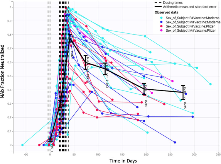
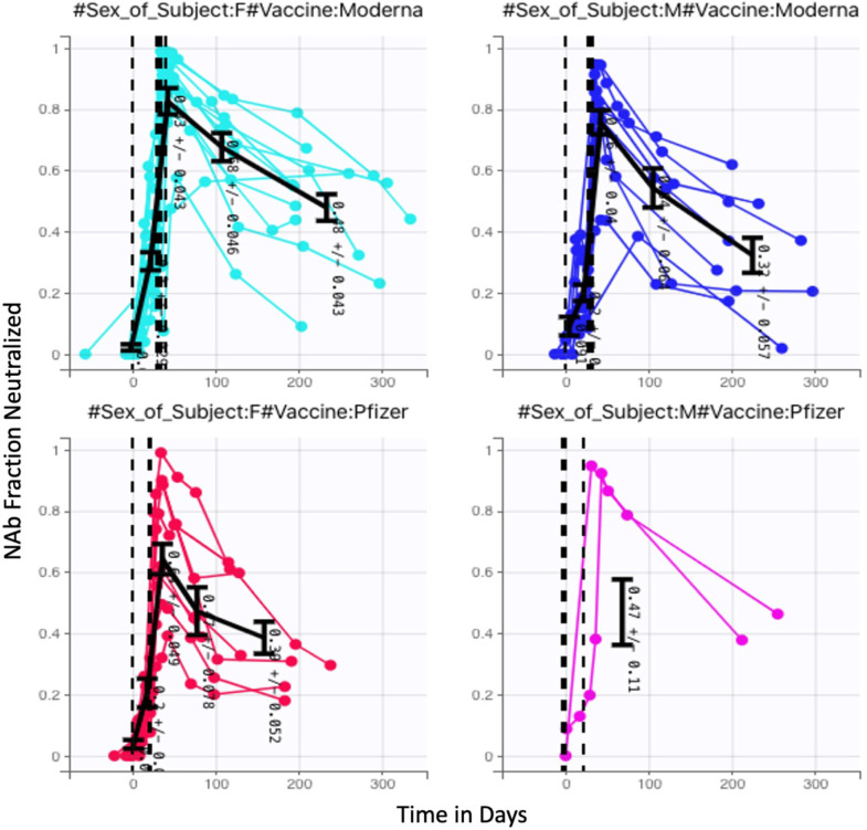
Time-series NAb data were collected through venous blood draws from 27 human subjects over a period of several months. Subjects included in this analysis were a subset of study participants enrolled in a prospective cohort study evaluating SARS-CoV-2 immune responses (NCT05379478), approved by WCG IRB (IRB $\#20202768$). At successive study visits at an Aditxt center in Mountain View, CA (MV), subjects with a history of COVID-19 vaccination provided blood (EDTA plasma) for determination of antibody profiles and neutralizing antibody activity. Each subject was, to the best of our knowledge, not previously infected with SARS-CoV-2, and each subject received two mRNA vaccine doses: some received two Pfizer doses, and some received two Moderna doses. From a sample of 27 subjects, 9 received Pfizer and 18 received Moderna. The number of samples, the number of days between samples, and the timing of the two vaccine doses varied from subject to subject. Once model development was completed and run on the 27 subject data sets, we further tested the model with NAb values from 5 additional subjects (1 received Pfizer, 4 received Moderna) and were able to achieve good fits without modification to the model. In the complete set of 32 subjects, 22 received Moderna and 10 received Pfizer. Additionally, 21 are female and 11 are male. The fraction neutralization time course data for all 32 subjects are pictured in Fig. 2, with colors assigned to distinguish between the results of Moderna and Pfizer vaccination, as well as between male and female subjects. Additional observations about this data set are in Appendix C.

Fig. 2.

Fractional neutralizing antibody activity: 32 Subjects, 22 Moderna (13 female, 9 male) 10 Pfizer (8 female, 2 male).

A deeper exploration of the data category differences is certainly of interest, but a thorough investigation would require a larger balanced data set, and is outside the scope of this paper. The focus of this work is on the development of a mathematical model for capturing within-host NAb time dynamics. The model fitting process, which is discussed in Section 3, showed that consideration of vaccine type or biological sex did not significantly impact model fits. With larger and better balanced data sets, however, this model may prove to be useful in the future for further exploring the differences between mRNA vaccine types and between biological sexes.

2.4. Mathematical model

The mathematical model we introduce is a two-state system describing NAb response to vaccine. The system of ordinary differential equations captures the high-level mechanistic dynamics of a vaccine-triggered immune response within an individual. Model states are:

• •$A$: Neutralizing antibody (NAb). Units: IU/mL
• •$V$: Proxy for transfected cells in response to mRNA vaccine. Units: mL

The dynamics of NAb over time are described by two nonlinear ordinary differential equations. The time scale is a 24 hour day:

$$\frac{dA}{dt}=r_{1}V+r_{2}AV+A\left(r_3-r_{4}A\right)$$ (1)

$$\frac{dV}{dt}=\alpha u\left(t\right)-\frac{k_{1}V}{(k_2+V)}$$ (2)

Here $\alpha u\left(t\right)$ represents a normalized vaccine dose in mL/day. The role of the vaccine dose in this model is simply as a trigger to engage an immune response; the model is not constructed to explore the effect of varying dosage levels. As discussed in Section 2.5.2, a sensitivity analysis showed that at a population level, the dosage parameter $\alpha$ had very little impact on model outcomes relative to the other model parameters, and that setting $\alpha =1$ for all subjects was sufficient to achieve model accuracy. State variable $V\left(t\right)$ in mL is a proxy for the activity of cells transfected as a result of vaccination. In a traditional dose–response model, an equation of this form would capture the pharmakokinetics of medication in the system, but mRNA vaccines behave differently, so $V$ is not the “amount of vaccine in the body”. Nonetheless, for the purposes of predicting antibody dynamics over time, the system as modeled reflects the initiation of the immune response with the saturation-limited clearance term conceptualized as “vaccine clearance”. Eq. (2) has the same form as the PK submodel presented in Eq. (1) in Tran et al. (2020) that captures drug concentration pharmacokinetics. As in the PK submodel of Tran et al. (2020), this form allows the vaccination to be administered at a time-dependent rate $u\left(t\right)$, and cleared at a Michaelis–Menten rate $\frac{k_{1}V}{(k_2+V)}$. Vaccine administration term $u\left(t\right)$ has units of mL/day. Since $u\left(t\right)$ is a proxy for the effect of vaccination, it does not represent the actual injection volume of either the Pfizer or Moderna vaccines. The presence of the transfected cells $V$ initiates an antibody response, represented by state variable $A\left(t\right)$. The dynamics of the antibody population within the individual, once triggered, are represented with a logistic term.

In particular, in Eq. (1):

• •$r_{1}V$ represents initiation of antibody activity in response to vaccine.
• •$r_{2}AV$ represents an antibody boost in response to vaccine.
• •$A\left(r_3-r_{4}A\right)$ models intrinsic antibody dynamics as logistic.

In Eq. (2):

• •$\alpha u\left(t\right)$ represents a vaccine dose that triggers the development of transfected cells. The time-dependent function $u\left(t\right)$ has units mL/day and is a discrete pulse with total input set to $1$ on the days vaccine is administered, and $0$ otherwise.
• •$\frac{k_{1}V}{(k_2+V)}$ is a Michaelis–Menten type decrease in transfected cells over time.

Table 2 lists all model parameters, along with units and descriptions.

Table 2.

Model parameters, units, and descriptions.

Parameter	Units	Description
$r_1$	IU/(day mL${}^2$)	Antibody initialization in response to vaccine dose
$r_2$	1/(day mL)	Increase in existing antibody in response to vaccine dose
$r_3$	1/day	Proportional to intrinsic antibody growth rate
$r_4$	mL/(day IU)	Proportional to intrinsic antibody decay rate and intra-species competition
$\alpha$	Unitless	Scaling of vaccination administration function $u\left(t\right).$
$k_1$	1/day	Michaelis–Menten scaling for clearance of $V.$
$k_2$	mL	Michaelis–Menten half-saturation.

Fig. 3.

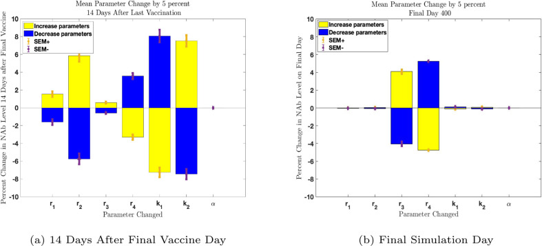
Parameter sensitivity analysis in MATLAB evaluating change in NAb levels resulting from a one-at-a-time 5% increase (yellow) and decrease (blue) in parameters. All 32 subject parameter sets were tested individually. Mean parameter changes with Standard Error of the Mean (SEM) are shown. Panel 3(a): Parameter sensitivity two weeks after second vaccine administration. Parameters $r_2,k_1,k_2$ are more influential than the remaining parameters at this time point. Parameter $\alpha$ is not influential. Panel 3(b): Parameter sensitivity on final day of simulation. Influence ranking has shifted so that parameters $r_3$ and $r_4$ now have the greatest effect on long-term outcomes. Parameter $\alpha$ remains non-influential.

2.5. Parameter fitting, sensitivity analysis, and numerical solution approach

For our investigations of parameter fitting and parameter influence, we ran a number of numerical experiments using both Monolix  (Lixoft SAS, Antony, France, 2021) for nonlinear mixed effects modeling (NLMEM), and MATLAB  (MathWorks) with MATLAB’s Global Optimization Toolbox (MathWorks, 2021). Global optimization computations with MATLAB achieve high accuracy when fitting model parameters to individual data sets, but computations can be very slow in practice. The nonlinear mixed effects modeling approach allows us to fit model parameters to individual subject data sets while also taking into account population-level trends. Subject-specific parameters are found by incorporating both within-subject and between-subject variability when fitting a model to data. Use of between-subject constraints may yield some individual fits to data that are less precise than those that can be achieved by separately fitting each subject data set without considering population-level information. A significant advantage to the NLMEM approach, however, is that when a data set for one subject alone is insufficient to compute individual parameters accurately, determining parameters in the context of the entire population can significantly reduce the level of uncertainty in the individual parameters, c.f., Bauer, 2019, Karlsson et al., 2015 and Bonate (2006). In addition, Monolix software is computationally efficient and provides a number of statistical tests that are helpful in exploring correlations between parameters as well as covariates, such as vaccine type and biological sex, that may influence model parameters. In light of the advantages to using NLMEM for fitting multiple subject data sets, we have not included MATLAB optimization outcomes in this paper, and instead have chosen to present model outcomes using parameter sets computed with Monolix.

Our parameter sensitivity analysis and the nonlinear mixed effects experiments informed the selection of which model parameters should be fit to each individual. We found that allowing all four parameters $r_1,\dots ,r_4$ of Eq. (1) to be subject-specific improved fitting outcomes and yielded biologically reasonable results. For the remaining three model parameters $\alpha ,k_1$, and $k_2$ in Eq. (2), we used Monolix to investigate whether fitting these parameters to each individual resulted in better fits than when we assigned fixed values. As stated, the function $V\left(t\right)$ of Eq. (2) represents the activity of transfected cells, and in its current form is not directly measurable. When considering the selection of the parameters of Eq. (2), therefore, we must prioritize capturing biologically reasonable behavior: a surge in response to vaccine administration, and clearance within a few weeks or less, a time frame that is consistent with that of currently understood spike protein decay rates  (Cognetti and Miller, 2021). The use of Monolix to explore selection of values for $k_1$ and $k_2$ is discussed in Section 2.5.1. We also performed a one-at-a-time sensitivity analysis in MATLAB to assess the influence of each model parameter. Both the Monolix experiments and the MATLAB sensitivity analysis showed that $\alpha$, which scales the vaccine administration function $u\left(t\right)$, is not an influential parameter and does not need to be fit to each individual. We therefore set $\alpha =1$ for all subjects, which was sufficient to achieve model accuracy. The sensitivity analysis also showed that parameters $k_1$ and $k_2$, which scale the Michaelis–Menten decay dynamics for state variable $V$, are more influential at earlier time points, and less influential than other parameters at later simulation times. As discussed in Section 2.5.2, our focus is on long term outcomes, so fine-tuning of the selected values for $k_1$ and $k_2$ is not necessary for addressing our modeling question.

2.5.1. Monolix population level parameter fitting

With Monolix  (Lixoft SAS, Antony, France, 2021) for computing nonlinear mixed effects on our structural model, we explored a number of statistical models, and investigated whether the population parameters $k_1,k_2$, and $\alpha$ would give better outcomes if fit to each individual. Using both a sensitivity analysis in MATLAB (see Section 2.5.2) and parameter fitting in Monolix, we confirmed that the parameter $\alpha$, which is used as a proxy for “dosage strength”, is not influential relative to other model parameters, most likely because function $u\left(t\right)$ does not represent vaccine volume but instead is an immune trigger activated by vaccine administration. Comparing various statistical models and using the Akaike Information Criterion (AIC) as a measure of goodness of fit, we found the statistical model we next describe yielded the best fit in combination with good outcomes for statistical tests.

Our structural model is our ODE system (1), (2). For the observation model, we used Monolix’s “constant” error model, in which a random error term with constant variance is added to our prediction of the NAb response. For the individual model, the transformations that yielded the best statistical outcomes were a logitnormal transformation for all four of the $r_i$ parameters. Allowing correlation between $r_1$, $r_2$, and $r_4$ also led to improved outcomes. Although our data set indicates there may be some differences in the NAb dynamics of Moderna-vaccinated and Pfizer-vaccinated individuals, as well as possible difference between male and female subjects, the inclusion of vaccine type and biological sex as covariates did not improve statistical outcomes or fits for any of the model parameters. Further details of Monolix’s implementation can be found in the Monolix documentation  (Lixoft SAS, Antony, France, 2021). We found that we could achieve a somewhat lower AIC when allowing $k_1$ and $k_2$ to vary by individual, but those fits led to model behavior that was not biologically justifiable; with individually fit $k_1$ and $k_2$, state variable $V\left(t\right)$ persisted at high values for the entire simulation. State variable $V\left(t\right)$ is a proxy for transfected cells which are meant to decay away within a few weeks, a time frame consistent with that of spike proteins  (Cognetti and Miller, 2021). Given our model assumptions that dosing function $u\left(t\right)$ does not represent vaccine volume, it is reasonable that the vaccine trigger effect be the same for all subjects. Assigning constant values to $k_1$ and $k_2$ led to biologically reasonable dynamics and appropriately rapid decay of $V\left(t\right)$ over time. We selected the values $k_1=10$ and $k_2=50$ by noticing a trend that when we allowed individual fitting, $k_2$ tended to be on the order of 5 times larger than $k_1$ in several cases.

2.5.2. Sensitivity analysis

The sensitivity analysis in MATLAB  (MathWorks) was initiated with individual parameter values found by Monolix for $r_1,\dots ,r_4$, and with fixed values $\alpha =1$, $k_1=10$, and $k_2=50$. A one-at-a-time analysis ran up and down shifts in all 7 parameters on all 32 subjects, and computed the mean responses. We extracted the ODE solutions at two time points: 14 days after the final vaccine administration, and on day 400, which is past the final day of our simulations. This sensitivity analysis indicates that $k_1$ and $k_2$ are more influential in the early time transient stage of the solution and less so at later times. More sophisticated uncertainty and sensitivity analysis techniques that employ Latin Hypercube Sampling, Sobol’s method, eFAST, or Multi-test-eFAST can be used, and may be of interest in future work, c.f., Marino et al., 2008, Renardy et al., 2021 and Dela et al. (2022).

For the question we are asking, the early time transient stage of the vaccine response is less important than that of the long term outcome. In the long term, the influence of $k_1$ and $k_2$ has waned. In addition, as discussed in Section 2.5.1, individually fitting $k_1$ and $k_2$ led to non-biological outcomes. We were able to achieve biologically reasonable and useful outcomes as well as good overall fits to data when keeping $k_1$, $k_2$, and $\alpha$ constant and individualizing only the four parameters $r_i$, $i=1\cdots 4$ of Eq. (1). We present a comparison of fitting outcomes in Section 3. A full list of parameter values used in the simulations is included in Appendix A.

2.5.3. Markov-chain Monte Carlo for generating prediction envelopes

Markov-Chain Monte Carlo (MCMC) methods can be used to enhance the process of fitting models to data. MCMC methods are sampling methods, and are not primarily used to find the best fit parameters to a particular data set. Optimizers such as those cited above are better choices for finding optimal parameter values. Starting with optimum parameter choices, MCMC produces a chain (a large set) of likely parameter combinations and generates a distribution of model outcomes by sampling parameter combinations from the chain. Using the package mcmcstat (Laine, 2019) for MATLAB, we ran MCMC on each subject’s data set to produce predictive envelopes for model outcomes. The mcmcstat package provides tools to generate and analyze Metropolis–Hastings MCMC chains using multivariate Gaussian proposal distribution (Haario et al., 2001, Haario et al., 2016). The parameter values found via Monolix Table 3 were used as initial parameter guesses. For our data sets, we set a burn-in time of 500 iterations, and generated an MCMC chain of length 5000. Predictive envelopes were determined by sampling the chain 1000 times, then determining predictive quartiles of $50\text{\%}$, $90\text{\%}$, $95\text{\%}$, and $99\text{\%}$.

2.5.4. Model simulations

Model simulations were run using a stiff ODE solver ode15s in MathWorks. The assay data provide results in percent neutralization, which ranges from $0$ to $100$. To increase numerical stability, the data were rescaled to range between $0$ and $1$. After solutions were computed and parameter values were found, results were then scaled up to units of IU/mL via the percent neutralization to IU/mL conversion function described in Section 2.1. This function can take on values between $0$ and $2200$.

3. Results

3.1. Individual subject outcomes: Immune protection stratification

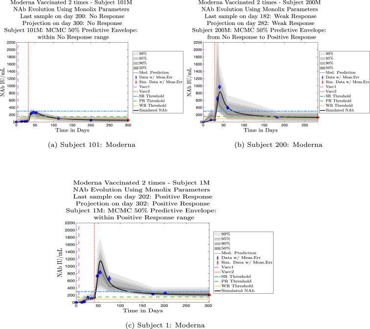
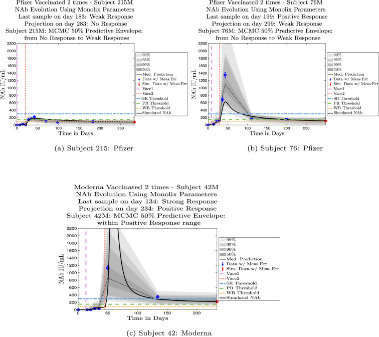
In Fig. 4, Fig. 5 we explore the immune protection categories to which an individual belonged at the time a subject’s last sample was taken, along with the immune protection category projected by the model simulation approximately 3 months after the final sample day. Model simulations are aligned so that the first day of each simulation is set to $0$. In Fig. 4, we show three examples of subjects whose immune categories are maintained three months after the final sample was collected. One subject remains in the no-response (NR) range, one maintains a weak response (WR), and one maintains a positive response (PR). In Fig. 5 are three examples of subjects whose immune categories are projected to drop over the three months following the collection of the final sample. One subject drops from a weak response to no response, one drops from a positive response to a weak response, and one drops from a strong response to a positive response. In general, we see a pattern of a subject’s projected immune protection over a three month period either matching that of the last sample, or dropping into a lower category. In the subject samples we have, final samples for the majority of the subjects were collected approximately six months after completion of the two-vaccine series. Individuals tended to drop by no more than one immune strength category 3 months after the final sample was collected.

Fig. 4.

Example subjects for whom the immune-strength category of the final data sample and on final projected day remains unchanged. Panel 4(a), Subject 101: Last sample and final simulation both show no response (NR). Subject remains in NR range on final simulation day. Panel 4(b), Subject 200: Last sample and final simulation both show weak response (WR). The boundaries of the 50% predictive envelope range from NR to PR on final simulation day. Panel 4(c), Subject 1: Last sample and final simulation both show a positive response (PR). Subject is predicted to remain within the PR range on final simulation day.

Fig. 5.

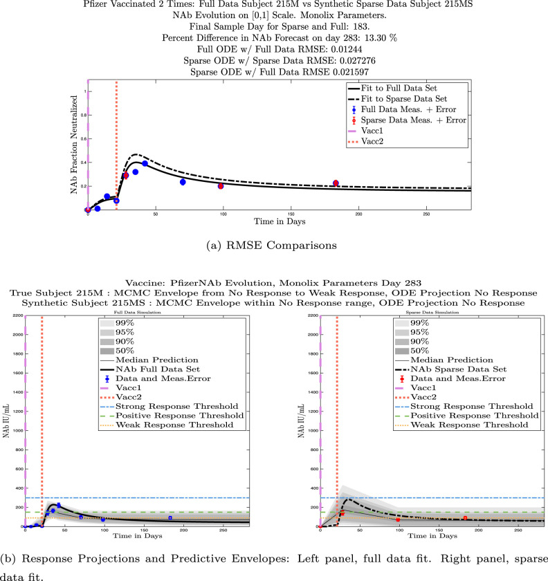
Example subjects for whom the projected immune-strength on the final simulated day drops one category relative to the immune strength category of the final data sample. Panel 5(a), Subject 215: Last sample shows a weak response (WR) but final simulation predicts no response (NR) 3 months later. The boundaries of the 50% predictive envelope range from NR to WR. Panel 5(b), Subject 76: Last sample shows a positive response (PR) but final simulation predicts a weak response (WR) 3 months later. The boundaries of the 50% predictive envelope range from NR to WR. Panel 5(c), Subject 42: Last sample shows a strong response (SR) but final simulation predicts a positive response (PR) 3 months later. The boundaries of the 50% predictive envelope are within the PR range.

3.2. Shared household married couples: Sex differences

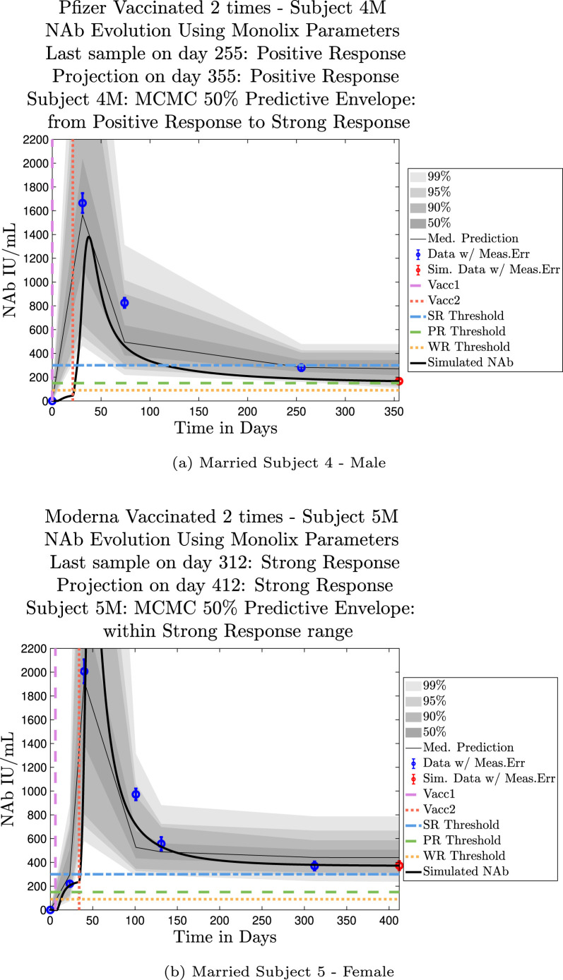
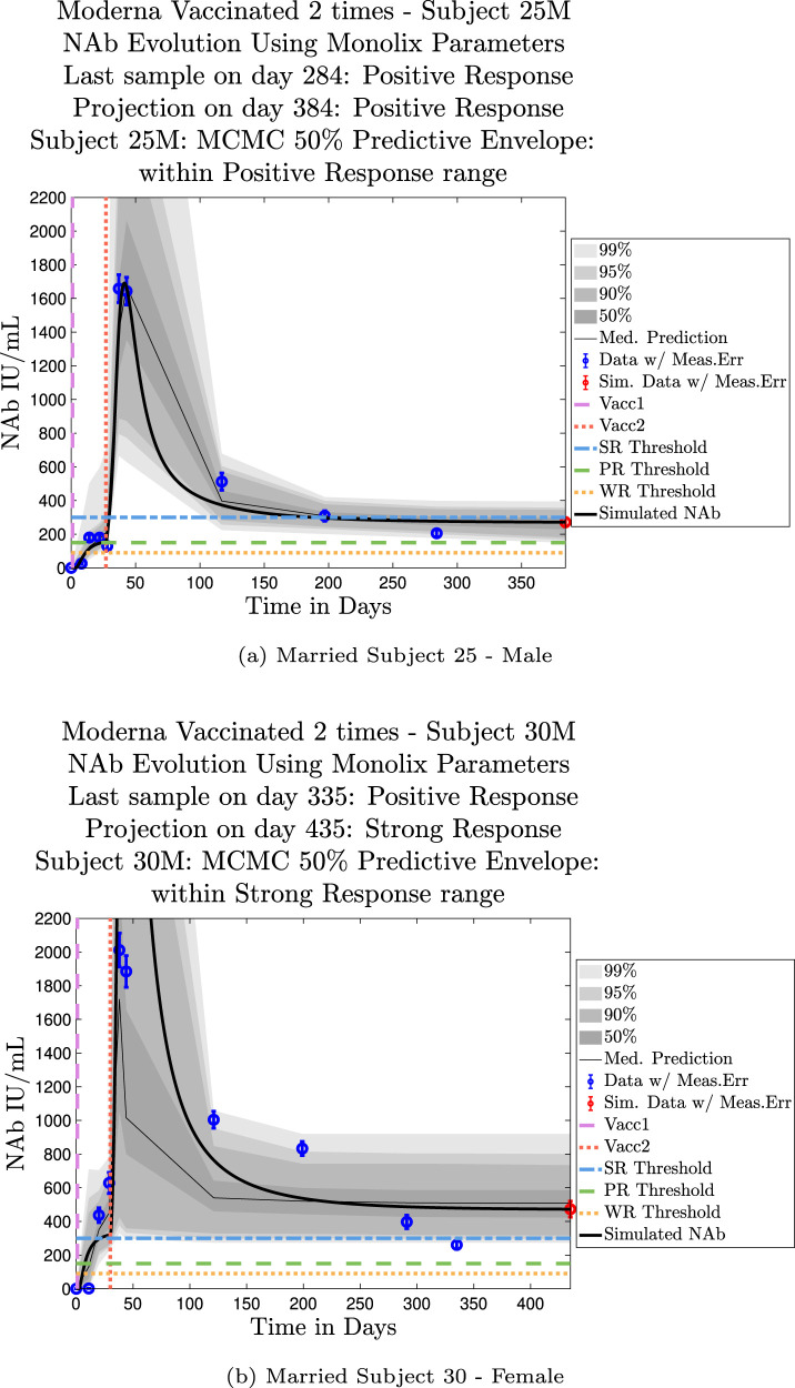
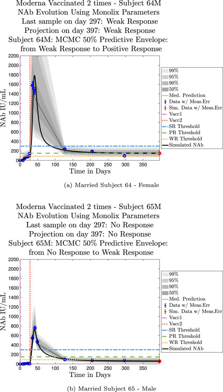
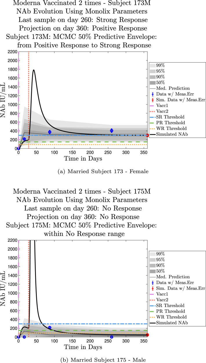
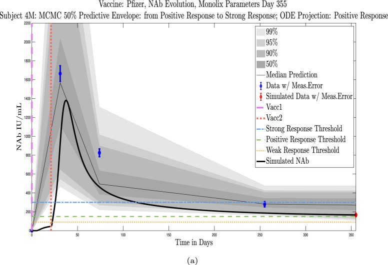
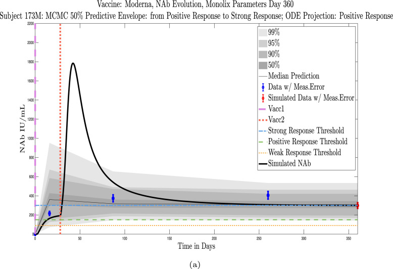
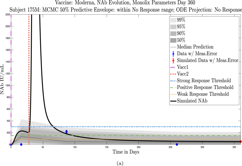
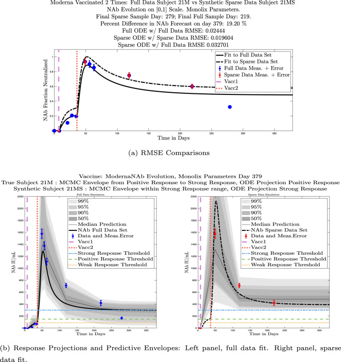
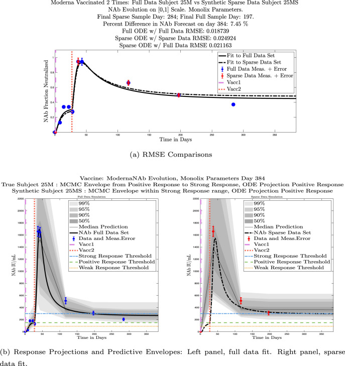
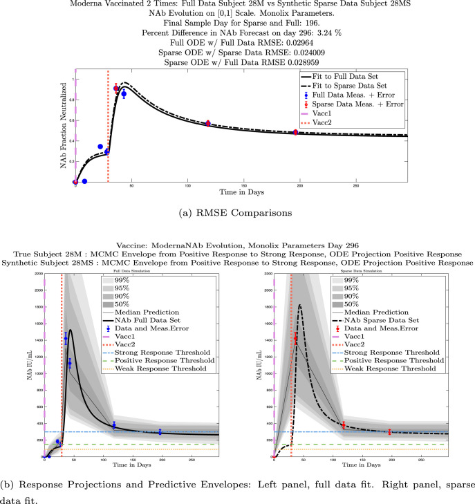
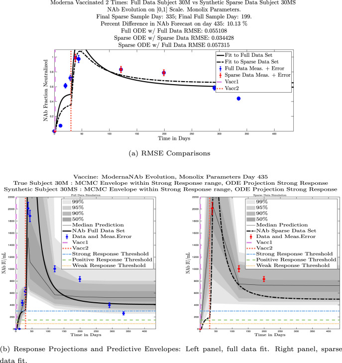
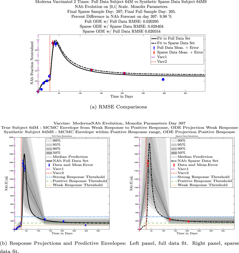
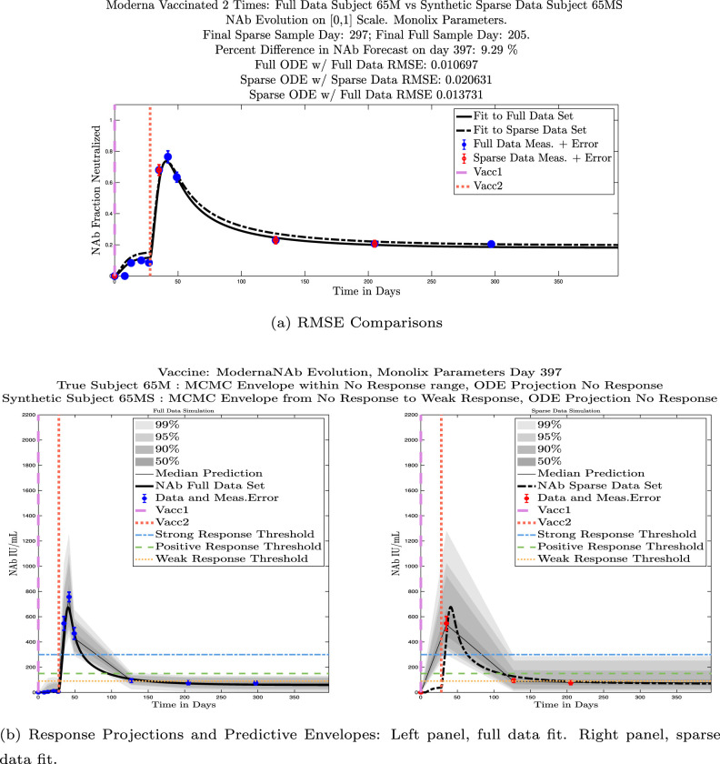
The cohort data set includes 5 male–female married couples. Understanding sex difference in response to vaccine can be complicated because of so many confounding factors that vary from individual to individual, including risks encountered via household practices, profession, and quality of adherence to safety protocols. Since these married couples live in the same household, one factor is normalized. The comparison within male–female married couples revealed a tendency in this small sample set for the overall strength of response of the female partner to be more robust than that of the male partner. In our data set, we saw one case (subjects 20 and 21) in which the early-time male response was slightly stronger than that of the female partner, but we saw no cases in which the male partner had a significantly stronger overall response than the female partner. On the other hand, in the majority of cases the female partner had a more robust response than the male partner. This observation is consistent with prior studies demonstrating stronger immune responses, and specifically stronger antibody responses to vaccines, in women, c.f. Fischinger et al. (2019). This distinction is clear when comparing individuals within married-couple pairs, but the sex difference is not as clear when these subjects are mixed back into the general population. Further discussion about biological sex differences within the general population can be found in Appendix C. In Fig. 6 comparing subjects 4 (male partner) and 5 (female partner), it is clear that both the initial response to vaccine and persistence over time is stronger in subject 5. One confounding factor in this case, however, is that subject 5 received the Moderna vaccine, but her partner, subject 4, received Pfizer. In Fig. 7, the difference in response between married subjects 20 and 21 is not as clear, and the male partner has a stronger early response, but the long-term 50% predictive envelopes indicate a similarly strong response in the female partner. In Fig. 8 it is apparent that subject 30 (female partner) has a stronger overall NAb response than does subject 25 (male partner). The difference in response is also distinct in Fig. 9 between subject 64 (female partner) whose initial response was much stronger than that of subject (65) male partner, and persistence is somewhat stronger as well. In Fig. 10, there are only two post-vaccination sample points, which introduces more uncertainty into simulated outcomes. Since no samples were collected until nearly three months after the final vaccination, the initial post-vaccine response of both subjects is inferred by the ODE solutions alone. Nonetheless, subject 173 (female partner) has a strong persistent response to vaccine whereas the response of subject 175 (male partner) has dropped to the no-response (NR) category both on the final sample day and on the last simulated day. The pattern of the stronger female response in the majority of married-couple cases indicates that further exploration of within-household responses may be warranted.

Fig. 6.

Married Subjects 4 (M), 5 (F): Male–Female comparison of response predicted through the final simulated day.

Fig. 7.

Married Subjects 20 (M), 21 (F): Male–Female comparison of response predicted through the final simulated day.

Fig. 8.

Married Subjects 25 (M), 30 (F): Male–Female comparison of response predicted through the final simulated day.

Fig. 9.

Married Subjects 64 (F), 65 (M): Female–Male comparison of response predicted through the final simulated day.

Fig. 10.

Married Subjects 173 (F), 175 (M): Female–Male comparison of response predicted through the final simulated day.

3.3. Model calibration with fewer data points

In this section we ask whether we can sample fewer data points and still produce useful model outcomes. We first explore whether an initial strong response to vaccine translates into strong NAb persistence over time (it does not). We then investigate whether using only three strategically-timed sample points after the second vaccination produces useful model fits (it does, in most cases).

3.3.1. Strong initial response versus persistence

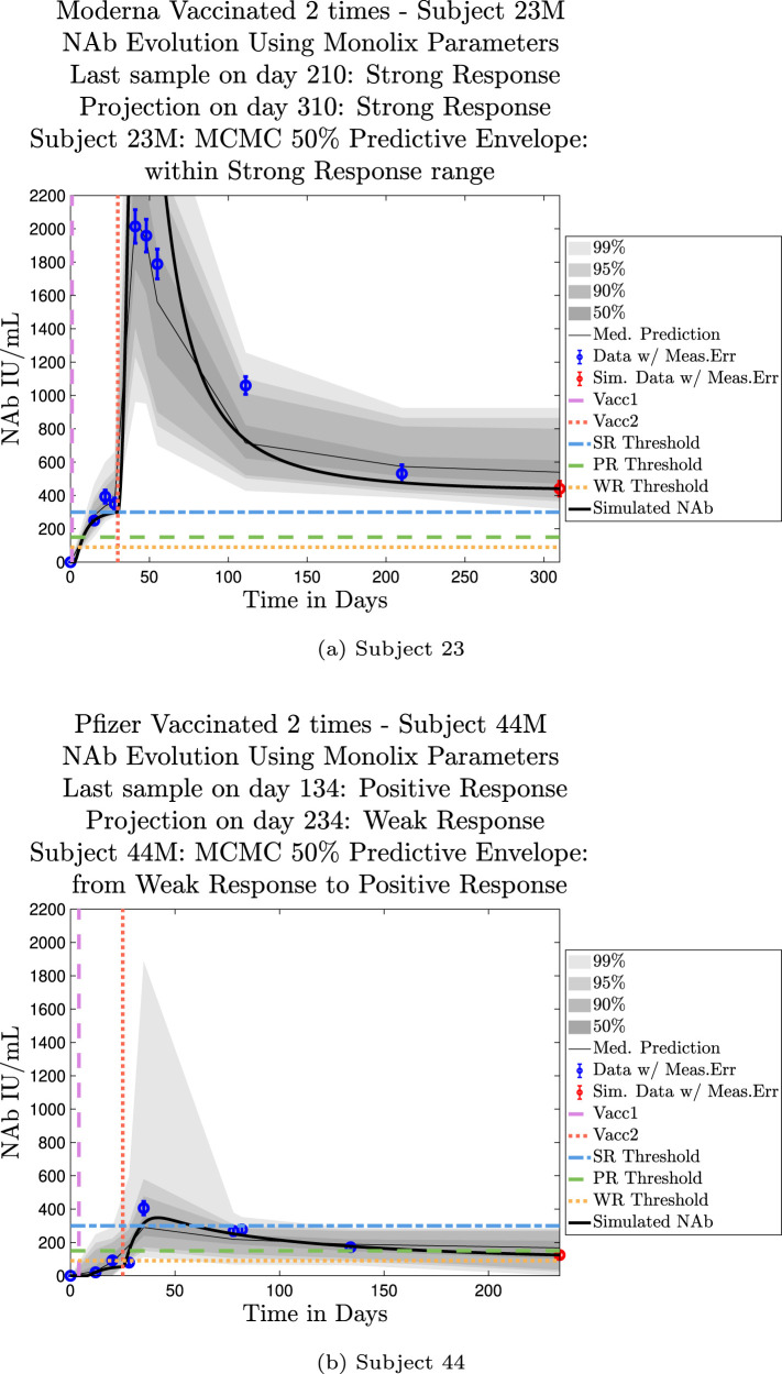
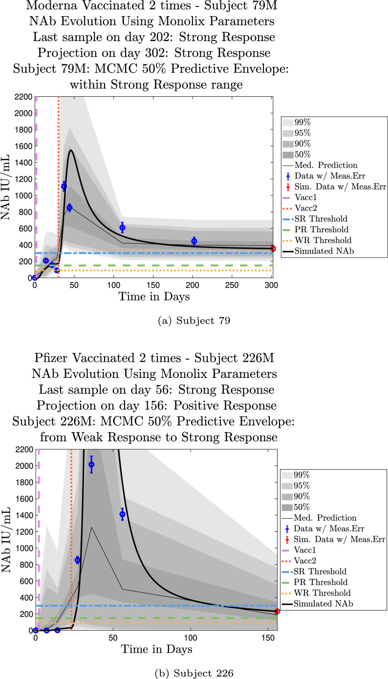
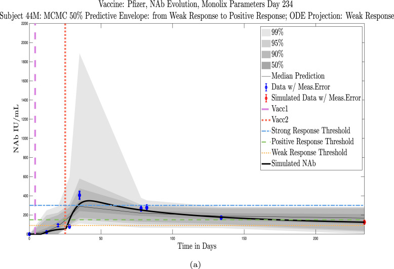
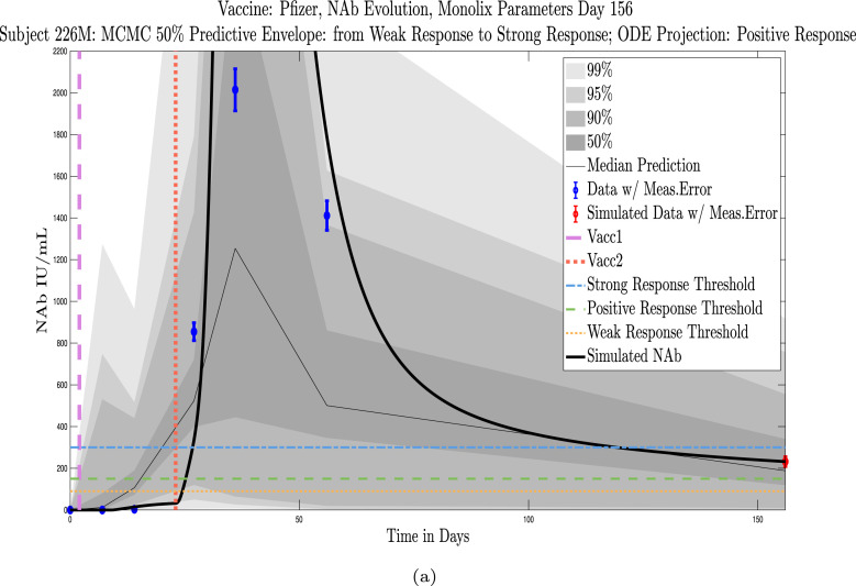
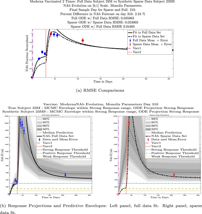
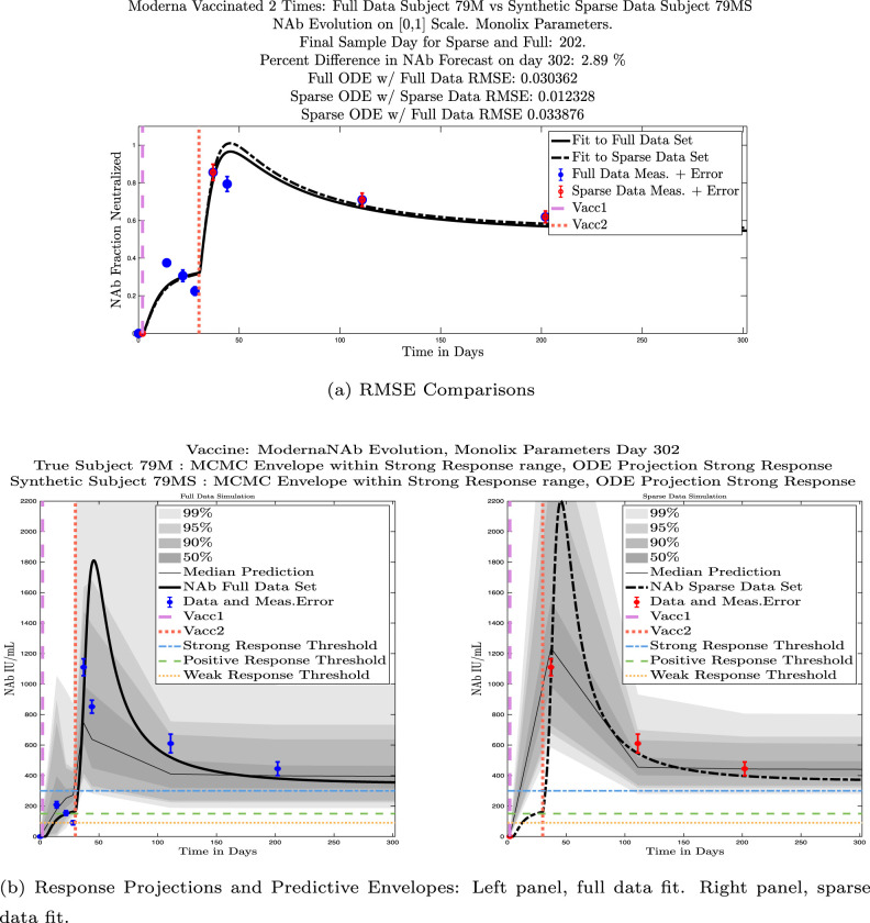
Model simulations show a fairly weak maximum NAb response to the first vaccine dose among nearly all individuals in the cohort, indicating at best low levels of protection after only one administration of the vaccine. The second vaccine dose shows a much stronger response, both in maximum NAb level and in persistence of higher levels. This behavior is captured by the model as a response to a vaccine challenge when there is preliminary immune system priming in place. In the data sets we analyzed, it was clear that an initially strong response to the second vaccine dose did not always predict high NAb levels over time. In certain cases, a strong response persisted, but in others, an initially strong response can be seen to decline to nearly no response several months later, whereas initial responses that are only moderate can persist. When the initial response is relatively weak, NAb levels remain low. Subjects 23 and 44 are examples of individuals for whom the initial response does predict long term behavior. Subject 23 in Fig. 11(a) shows a very robust initial response to the second vaccine dose, and by the final simulated day, NAb levels remain above the strong response threshold. Subject 44 in Fig. 11(b), on the other hand, shows a weak initial response to the second vaccine dose, and as expected, by the final simulated day, the response has dropped below the weak response threshold. The pattern of persistence we see in subjects 23 and 44, however, is not a pattern seen in all subjects. While a weak initial response is a good indicator that the response will remain weak, a strong initial response does not necessarily guarantee persistence of high levels of NAbs in an individual over time. When we compare subjects 79 in Fig. 12(a) and 226 in Fig. 12(b), we see that the stronger initial response of 226 does not guarantee stronger persistence. We also note that the predictive envelopes for these two subjects cover much broader ranges than do the envelopes for subjects 23 and 44. Subject 226, in particular, has a 50% predictive envelope on the final simulated day that covers all response thresholds from weak to strong. The best fit simulation, however, projects that NAb levels in subject 226 will have declined to the weak response category 3 months after the final sample.

Fig. 11.

Predictive envelopes with best fit curve. Subjects 23 and 44: Strong and weak initial responses correspond to long-term high and low NAb levels, respectively. A very strong initial response in subject 23 to the second vaccine dose persists with strong protective immunity over time. A relatively weak initial response in subject 44 to the second vaccine dose continues to show weak protective immunity over time.

Fig. 12.

Predictive envelopes with best fit curve. Subjects 79 and 226: Stronger initial responses do not predict stronger long-term protective immunity over time. A moderate initial response in subject 79 to the second vaccine dose persists with strong protective immunity over time, and the 50% predictive envelope is within the strong response (SR) range. A very strong initial response in subject 226 to the second vaccine dose declines to positive protective immunity (PR) over time, and the 50% predictive envelope even allows for a weak response by the last projected day.

3.3.2. Sparse sampling hypothesis

In our data set, most of the subjects were able to supply samples at frequent time intervals, which was helpful in getting a good picture of general NAb dynamics over time. In practice, people may be less willing to supply blood samples as frequently, so we explored the question of whether it is still possible to get useful model fits with fewer data samples. As discussed in Section 3.3.1, it may seem intuitive to assume that a strong initial NAb response to vaccination would predict a persistent NAb response over time, but we saw counter-examples to this (subjects 79 and 226 were such examples). It is therefore clear that one post-vaccine data point is not sufficient to predict the long-time NAb dynamics within an individual.

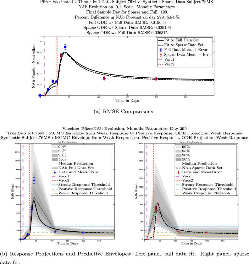
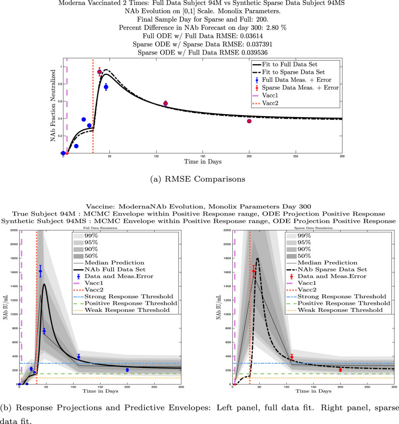
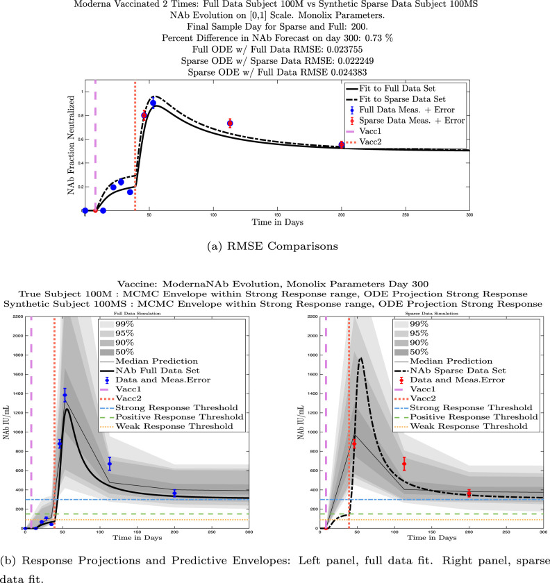
In ongoing Aditxt studies, new subjects who are currently enrolling are being asked to submit samples about two weeks after the final vaccination and subsequently at 3 month intervals. This led us to investigate what we are calling our “sparse sampling hypothesis”: the idea that with samples collected at only three strategically-timed post-vaccination points, our model can produce outcomes that closely mirror outcomes produced using larger sets of more frequently sampled data. We investigated this hypothesis by evaluating model solutions with fits that were constrained to using only post-vaccination data points that were collected at times that align with current study guidelines: two weeks, 3 months, and 6 months after the second vaccination. Although, as we have seen, the strength of the initial response alone is not sufficient to predict long-term NAb levels, we do see evidence from this subject data set that taking samples at the currently recommended time intervals produces results that are well-aligned with results produced when using more frequently collected samples. We performed numerical experiments by creating “synthetic” subjects out of our real subjects by creating a subject “twin” with the constraint that the synthetic twin uses only three of the post-vaccine data samples. That is, given the time series data from an individual with four or more post-vaccination data points, we extracted just the 3 points sampled around 2 weeks, 3 months, and 6 months after vaccination, and re-ran the model fits with Monolix. Of our 32 original subjects, there are 21 who have more than four post-vaccination samples with a subset of the samples collected at times within the desired timeframes. We present comparisons between sparse data and full data model fits and projections using these 21 “real/synthetic” pairs.

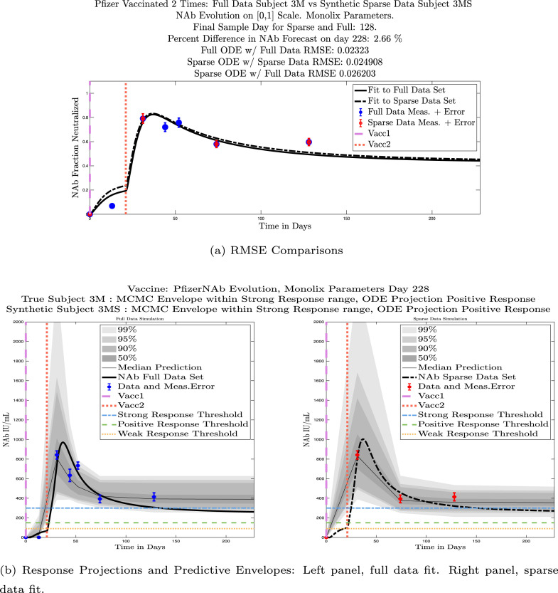
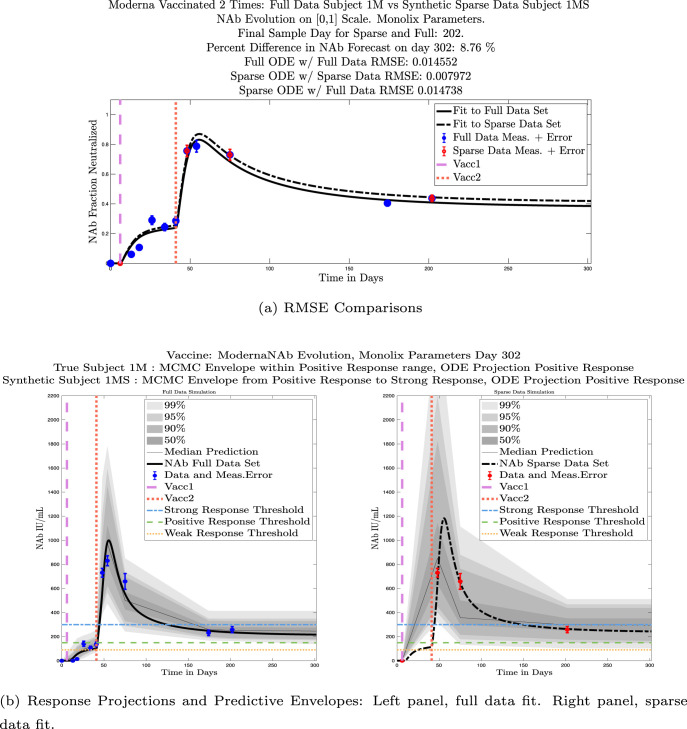
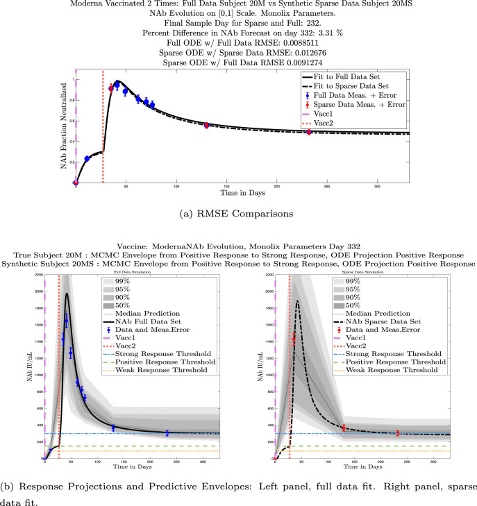
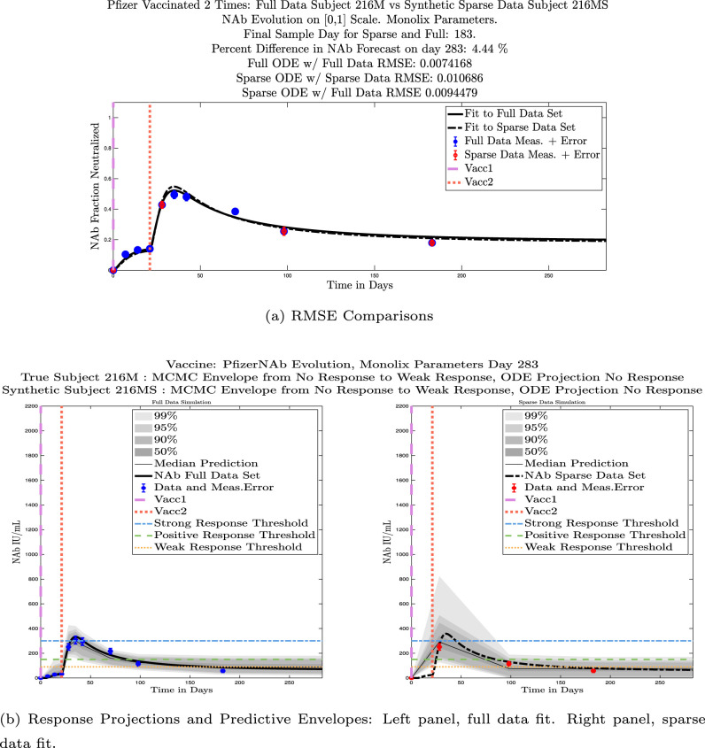
In Fig. 13, we show the “real/synthetic” comparison for subject 3. Subject 3 has 6 associated data points. We plotted “3M” alongside “3MS”. Here, the label “M” designates the Monolix fit using the full set of data points, and “MS” designates the “synthetic” subject fit by Monolix using only the sparse subset of data points. In panel 13(a) we see the ODE solutions fit to the full data set (solid line) and the sparse data set (dashed line) plotted on top of each other. The sparse data subset used to fit the dashed line is highlighted in red. In this example, we see that 3 months after the final sample was collected, the difference in the NAb values computed by the full-fit and sparse-fit ODEs is less than $3\text{\%}$. As one measure of numerical goodness-of-fit, the computed root mean squared errors (RMSE) are also printed for comparison. The case “Full ODE w/ Full Data” is the RMSE computed when comparing the differences between the full data set (in blue) and the ODE fit to the full data set (solid line). The case “Sparse ODE w/ Sparse Data” is the RMSE computed when comparing the differences between the sparse data set (in red) and the ODE fit to the sparse data set (dashed line). Finally, the “Sparse ODE w/ Full Data” measure is the RMSE computed when comparing the differences between the full data set (in blue) and the ODE fit to the sparse data set (dashed line). For subject 3, the RMSE of the “Full ODE w/ Full Data” case (ODE fit with 6 data points) is about 0.02323, and the RMSE of “Sparse ODE w/ Full Data” case (ODE fit with only 3 data points) is 0.026203, a difference of less than 0.003.

Fig. 13.

Full-data fit by Monolix compared to sparse-data fit by Monolix. In panel 13(a), solutions are plotted on a normalized [0,1] scale indicating the fraction of virus inhibition. The three post-vaccine data points are a subset of the full data set and are highlighted in red. Also shown is the percent difference between the full-data fit and the sparse-data fit in final NAb level forecast, as well as the root-mean-squared errors (RMSE) for the following scenarios: ODE solution fit with full data compared to full data set; ODE solution fit with sparse data compared to sparse data set; ODE solution fit with sparse data compared to full data set. In panel 13(b), the ODE solution and the MCMC prediction envelopes for the full-data fit and sparse-data fit are plotted side-by-side on an IU/mL scale. In both scenarios, 3 months after the final sample point was collected, the 50% predictive envelopes are within the strong response (SR) range, the 99% envelopes cover the positive response (PR) to strong response (SR) ranges, and a positive protective immune response for this subject (PR) is forecast.

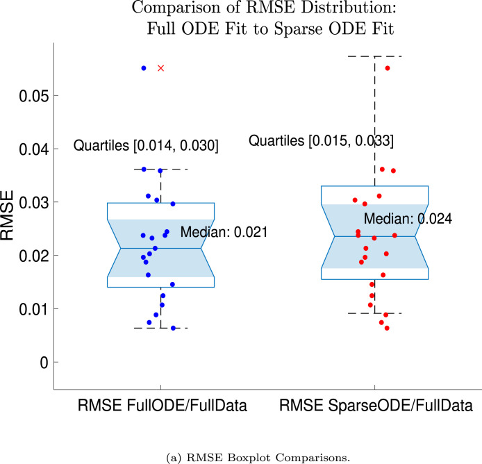
We ran the same comparisons for all 21 Full-Sparse (i.e., real-synthetic) pairs. The comparison plots for all 21 pairs are included in the Appendix. In Fig. 14 we summarize the RMSE comparisons for the entire set of 21 Full-Sparse subject pairs with a boxplot. We compare the RMSE measures for the full data set against the ODE fit to full data (labeled $M_{RMSE}$) and the RMSE measures for the full data set against the ODE fit to sparse data (labeled $M{S}_{RMSE}Fulldata$). We see that the distributions of the RMSEs in these two cases are similar. The median Full-ODE/Full-Data RMSE is 0.021, with 50% of the RMSE values between 0.014 and 0.03. The median Sparse-ODE/Full-Data RMSE is 0.024, with 50% of the RMSE values between 0.015 and 0.033. We ran a simple two-sample paired permutation test with $10,000$ permutations. In this case, the magnitude of the estimated mean RMSE difference is 0.0030 with a $p$-value of 0.0001. The small $p$-value indicates that the nonzero difference in the mean RMSEs is statistically significant. For our purposes, however, the RMSE difference is sufficiently small to conclude that the sparse sample fit still provides useful outcomes. We also ran a two-sample unpaired permutation test, also with $10,000$ permutations. The magnitude of the estimated mean RMSE difference is still 0.0030, but with this test the $p$-value is 0.4084, which means that if we treat the samples as independent, then the difference in means between the full-data and sparse-data group is not significant.

Fig. 14.

Population distribution of RMSEs across 21 full-sparse pairs: ODE fit to full data compared to full data set and ODE fit to sparse data compared to full data set. In the boxplot the central mark indicates the median, and the bottom and top edges of the box indicate the 25th and 75th percentiles, respectively. The whiskers extend to the most extreme data points not considered outliers. RMSE data are plotted with the “$•$” symbol.

We also compared projected response strength categories. Individual response strengths are provided in every plot in Appendix D, Appendix E, and are also listed in Table 3. In all but two cases, the projected response strength categories were identical. The two exceptions were subjects 21 and 64. For subject 21, the full-fit forecasts a positive response 3 months after the final sample point was taken. The associated sparse-fit forecasts a strong response. It is interesting to note, however, that the full-fit projection is very close to the strong-response threshold. In the case of subject 64, the full-fit forecasts a weak response, and the sparse-fit forecasts a positive response. Once again, the full-fit projection lies very close to the positive response threshold.

With only these 3 post-vaccine samples, the ODE model generates NAb curves and prediction envelopes that are well-aligned with the curves and prediction envelopes of the same subject with all data points included. Future work could involve applying optimal control theory to help determine ideal time intervals and the minimum number of samples needed to produce useful simulation outcomes.

4. Discussion

Our new mathematical model tracks levels of subject-specific neutralizing antibodies within an individual over time. Starting with 27 sets of longitudinal NAb level data from twice-vaccinated individuals, we developed our model to simulate NAb level changes in IU/mL to help predict the subject-specific within-host dynamics of antibody decay. Once the model was developed and tested on the 27 data sets, we tested the model on 5 additional longitudinal NAb level data sets, giving us a total of 32 data sets on which we ran the model. The model is sufficiently simple to be tractable, and can provide a high-level view of changing NAb levels within a specific host by fitting only four parameters to individual subject data. One of the advantages of the novel AditxtScore™ flow cytometry assay is that one can run more assays for less cost, thereby making the collection of longitudinal subject data easier. The availability of subject-specific data from this type of assay makes the implementation of our model practical. The model is phenomenological-mechanistic: phenomenological in how it captures the general dynamics of the vaccination trigger, and mechanistic in that the parameters for NAb level changes can be connected to biological meaning. The model state representing the action of an mRNA vaccine serves as a proxy for transfected cells. The model state representing the levels of NAbs in a system in IU/mL is a proxy for the neutralizing strength of the NAbs present in the system. The timing of the delivery of first and second vaccine doses varies from individual to individual. Even the with non-uniform collection of the number of samples and timing between samples, and the varying time gaps between the first and second vaccine administration for each subject, the model has sufficient flexibility to be able to achieve good fits to subject data. We applied NLMEM in Monolix to the 32 data sets to determine subject-specfic parameter values, and the MCMC sampling method in MATLAB to generate predictive envelopes. Each subject data set has between four and eleven time points at which NAb levels were measured. We also carried out model fitting with MATLAB’s Global Optimization Toolbox (results not pictured). The NLMEM approach yielded overall very good fits to subject data as measured by the RMSE.

The model is simple yet sufficiently complex to be able to capture a range of dynamics evidenced in the cohort of 32 subjects. Our analysis brought to light some NAb dynamic patterns worth noting. The first of these is a connection between married couples in the same household, which showed a tendency for the female partner to have a more robust NAb response than the male partner. The second is an observation that although a relatively weak initial response to a second vaccine dose tends to predict weak persistence of NAb levels over time, strong responses do not necessarily guarantee strong NAb persistence. Third, we showed that we could reduce the number of sample points used for ODE fitting to only three strategically timed post-vaccine samples and still capture useful outcomes. These patterns could be explored more deeply once more subject data sets are collected.

4.1. Future directions

Vaccine efficacy for immunity against infectious agents is primarily assessed in clinical studies designed to evaluate reduction in disease incidence compared to placebo. Determination of differences between subjects that receive the active product versus placebo requires a large sample size, which extends the time and cost required for vaccine development. The ability to enroll a high number of subjects in these clinical trials is easier when infection rates are prevalent in pandemic conditions; however, subject recruitment becomes more challenging in the absence of a pandemic. Furthermore, clinical studies are not ethically feasible if the pathogen is extremely virulent and/or deadly. Finally, observation of changes in the incidence of infection may not provide information on the level of protective immunity for each individual subject. Immunity status is not all or nothing and can be impacted by a variety of factors including viral load and replication rate, level of initial immune response elicited by the vaccine, which may vary from one individual to another, time from immunization, mode of immunization, and other factors. Identification of a correlate of protection can reduce the number of subjects and evaluation time needed for clinical trials. A correlate of protection can also provide information about individual immune responses.

The purpose of this study was to select a correlate, neutralizing antibody (NAb), that has been reported in the literature as a measure of protection, and to create a mathematical model to determine its trajectory over time. This mathematical model can potentially help determine the rate of decay of NAb levels in individuals as well as responses in a population. The model was able to achieve good fits to individual subject data sets, even though there was significant individual variability in NAb dynamics, including in the strength of response to vaccine and persistence of NAb levels. We saw that long-term NAb persistence could not necessarily be predicted by the strength of the initial NAb level increase immediately following a second vaccine dose. Khoury and coworkers (Khoury et al., 2021) used NAb levels in individuals who had convalesced from SARS-CoV-2 infection and individuals who received one of 7 commonly used COVID-19 vaccines to estimate the likelihood of protection. Using their findings as a starting point, we established multiple cut-points in NAb levels using a novel flow-cytometry-based test. Multiple cut points were identified to categorize NAb levels as none to minimal, weak protective response and strong protective response against the wild type virus. We analyzed the decay rate of NAb in 33 subjects who had no known history of SARS-CoV-2 infection and who had been fully vaccinated with two doses of the Moderna or Pfizer mRNA vaccines, and hypothesized protective immunity status using these cut points. While these cut points are meant to serve as guidelines to categorize the levels of NAb at a given time with respect to likelihood of protection, the levels required for protection may be impacted by the SARS-CoV-2 variant. Future studies are planned to test the model in different cohorts and with different SARS-CoV-2 variants, as well as to correlate the protective levels with incidence of breakthrough infections. Once the model has been tested in the context of these additional scenarios, we see several potential model applications, including more rapid evaluation of immune responses to vaccination to reduce time and expense of vaccine development; determination of immune responses on a case by case basis to identify vulnerable populations; and, more accurate assessment of the timing of boosters, again on a personalized level.

CRediT authorship contribution statement

Lisette dePillis: Conceptualization, Methodology, Mathematical model creation, Software, Numerical experiments, Validation, Formal analysis, Writing original draft, Writing – review & editing, Visualization, Project administration. Rebecca Caffrey: Validation, Formal analysis, Investigation, Review and editing. Ge Chen: Neutralizing antibody test development, Manuscript draft review. Mark D. Dela: Writing – review & editing. Leif Eldevik: Conceptualization, Investigation, Writing – review & editing. Joseph McConnell: Investigation, Writing – review & editing. Shahrokh Shabahang: Neutralizing antibody test development, Project conceptualization, Manuscript draft review. Stephen A. Varvel: Conceptualization, Investigation, Writing – review & editing.

Declaration of Competing Interest

The authors declare the following financial interests/personal relationships which may be considered as potential competing interests: LdeP and MDD have provided consulting services to Aditxt Therapeutics, Inc. GC, RC, LE, JM, SS, and SV have a financial interest in Aditx Therapeutics, Inc., including employment and stock.

Appendix A. Parameter values, vaccine type, biological sex

See Table 3.

Table 3.

Subject-specific parameter values for Eq. (1), computed via Monolix. Fixed parameter values for Eq. (2): $\alpha =1;$$k_1=10$$k_2=50.$ Sex is indicated with F (female) and M (male). The projected long-term response of each subject is shown in the rightmost column. If a subject has a synthetic sparse-data twin, the long-term response of the synthetic twin is shown in parentheses. Response strength key: NR = no response. WR = weak response. PR = positive response. SR = strong response.

Table 4.

Precision of method to determine AditxtScore™ for neutralizing antibodies (NAb) to SARS-CoV-2, given in 50 IU/mL intervals. Precision is inversely proportional to IU/mL.

Avg. IU/mL	Avg. $\text{\%}$CV
50	16.9
100	13.7
150	11.8
200	10.4
250	9.4
300	8.5
350	7.8
400	7.2
450	6.6
500	6.1
550	5.7
600	5.3
650	4.9
700	4.6
750	4.2
800	3.9

Appendix B. Precision of method for determining subject NAb levels in IU/mL

To quantify the precision of the method for determining NAb IU/mL based on the percent inhibition AditxtScore™ assay for neutralizing antibodies to SARS-CoV-2, we ran the precision on 4 subjects with 4 different IU/mL values, 6 assays per day, for 3 days. Fig. 15 shows a log-fit to the data. Interpolated percent variation values, based on the log fit, are in Table 4, given at 50 IU/mL intervals.

Fig. 15.

Approximate relationship between $\text{\%}$ CV as measured by the AditxtScore™ test for neutralizing antibodies to SARS-CoV-2 and NAbs in IU/mL.

Appendix C. Data categories: Vaccine type and biological sex

In Fig. 16, we decompose the NAb level data from the 32 subjects into vaccine-type and sex categories: Female-Moderna, Male-Moderna, Female-Pfizer, Male-Pfizer. Using the immune-strength response categories outlined in Section 1.2 (no-response (NR), weak-response (WR), positive-response (PR), and strong-response (SR)), we also show in Fig. 17 the final immune strength categories by percentage, comparing Moderna to Pfizer, and female to male. In Fig. 17, Panels Fig. 17, Fig. 17, we see that 45% of Moderna subjects maintained a strong immune response, compared to only 20% of Pfizer subjects who fell into the strong-response category. In Panels Fig. 17, Fig. 17, we see that 43% of the female subjects remained in the strong response category, while only 27% of the male subjects maintained a strong response.

Fig. 16.

Fractional neutralizing antibody activity: 21 female subjects in left column (top left 13 received Moderna, bottom left 8 received Pfizer), 11 male subjects in right column (top right 9 received Moderna, bottom right 2 received Pfizer).

Fig. 17.

Immune protection category of final NAb sample: Panel 17(a) 22 Moderna Subjects, Panel 17(b) 10 Pfizer Subjects; Panel 17(c) 21 Female Subjects, Panel 17(d) 11 Male Subjects.

This data set does point to the possibility of differences in the time-course behaviors between Moderna and Pfizer vaccinated subjects and between male and female subjects. The sex differential is not definitive, however. The pie charts in Fig. 17, Fig. 17 show a clearly stronger response by the final sample time in female subjects than in male subjects, and the top row of Fig. 16 could indicate that Moderna-vaccinated females have stronger overall response than Moderna-vaccinated males. The bottom row of Fig. 16, however, shows that the Pfizer-vaccinated male subjects have a more robust response than do the Pfizer-vaccinated female subjects. We must be cautious with drawing general conclusions from these observations. The sizes of the subsets in the sample set may be too small to assert definitively that the population trend differences seen here reflect true trends in the larger population. In addition, the set is not balanced with respect to vaccine type and sex: there are more than twice as many Moderna-treated individuals as there are Pfizer-treated individuals, and there are nearly twice as many female subjects as there are male subjects. Finally, there are likely a number of confounding factors with respect to household environment and lifestyle that make it difficult to make accurate assertions about differences between individuals in different vaccine and sex categories. Nevertheless, in Section 3.2, we compare the outcomes of male–female pairs from this data set who are married and who live in the same household, a comparison that at least removes the confounding factor of household environment.

Appendix D. Simulation plots — ODE solution fits with MCMC predictive envelopes

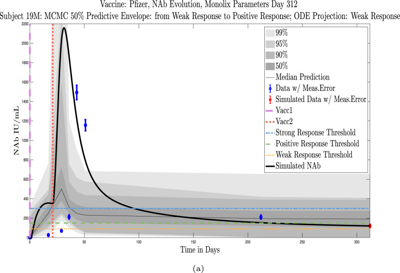
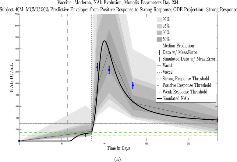
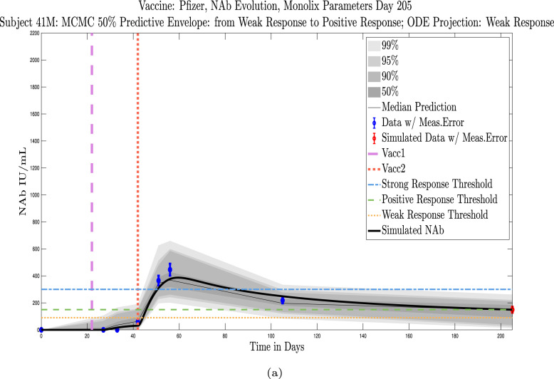
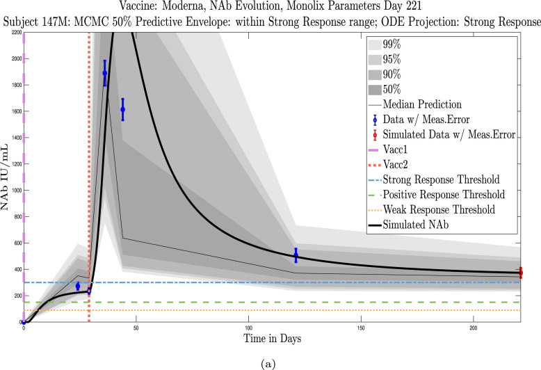
Shown in Appendix D, Appendix E are simulations for all 32 subjects using parameters fit with Monolix’s NLMEM software, superimposed on plots of the MATLAB-generated MCMC predictive envelopes for each subject. The ID numbers for the 11 subjects in this section who were not used to test the sparse sampling hypothesis are 4, 5, 19, 40, 41, 42, 44, 147, 173, 175, 226. Immune-strength thresholds are superimposed on the plots of ODE solutions and MCMC predictive envelopes. For each subject we have also identified the immune strength category in which the subject is forecast to be three months after the final sample was collected. (See Fig. 18, Fig. 19, Fig. 20, Fig. 21, Fig. 22, Fig. 23, Fig. 24, Fig. 25, Fig. 26, Fig. 27, Fig. 28).

Fig. 18.

Subject 4, Pfizer, Male.

Fig. 19.

Subject 5, Moderna, Female.

Fig. 20.

Subject 19, Pfizer, Male.

Fig. 21.

Subject 40, Moderna, Female.

Fig. 22.

Subject 41, Pfizer, Female.

Fig. 23.

Subject 42, Moderna, Male.

Fig. 24.

Subject 44, Pfizer, Female.

Fig. 25.

Subject 147, Moderna, Female.

Fig. 26.

Subject 173, Moderna, Female.

Fig. 27.

Subject 175, Moderna, Male.

Fig. 28.

Subject 226, Pfizer, Female.

Appendix E. Simulation plots — Full-sparse data fitting comparisons

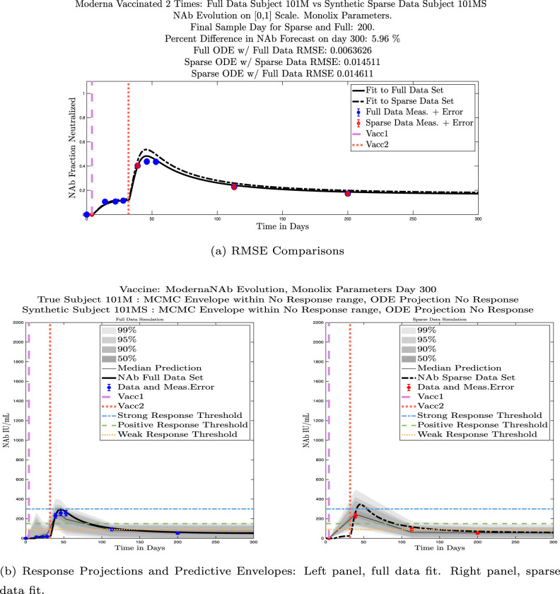
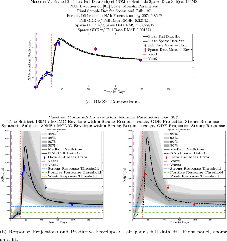
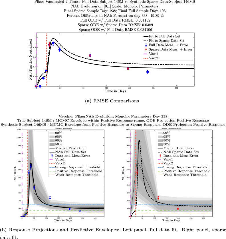
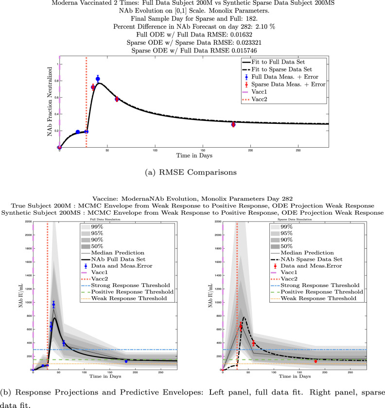
The ID numbers for the 21 subjects used to test the sparse sampling hypothesis are 1, 3, 20, 21, 23, 25, 28, 30, 64, 65, 76, 79, 94, 100, 101, 139, 146, 179, 200, 215, 216. In the associated figures, comparisons with the sparse-data fit ODE solutions are provided, including RMSEs of the full-data and sparse-data fits. Immune-strength thresholds are superimposed on the plots of ODE solutions and MCMC predictive envelopes for both the full-data real subject and the sparse-data synthetic twin. For each subject (both real and synthetic) we have also identified the immune strength category in which the subject is forecast to be three months after the final sample was collected. (See Fig. 29, Fig. 30, Fig. 31, Fig. 32, Fig. 33, Fig. 34, Fig. 35, Fig. 36, Fig. 37, Fig. 38, Fig. 39, Fig. 40, Fig. 41, Fig. 42, Fig. 43, Fig. 44, Fig. 45, Fig. 46, Fig. 47, Fig. 48, Fig. 49).

Fig. 29.

Moderna, Female. Full-data and sparse-data Monolix fits and MCMC predictive envelopes compared.

Fig. 30.

Pfizer, Female. Full-data and sparse-data Monolix fits and MCMC predictive envelopes compared.

Fig. 31.

Moderna, Male. Full-data and sparse-data Monolix fits and MCMC predictive envelopes compared.

Fig. 32.

Moderna, Female. Full-data and sparse-data Monolix fits and MCMC predictive envelopes compared.

Fig. 33.

Moderna, Female. Full-data and sparse-data Monolix fits and MCMC predictive envelopes compared.

Fig. 34.

Moderna, Male. Full-data and sparse-data Monolix fits and MCMC predictive envelopes compared.

Fig. 35.

Moderna, Female. Full-data and sparse-data Monolix fits and MCMC predictive envelopes compared.

Fig. 36.

Moderna, Female. Full-data and sparse-data Monolix fits and MCMC predictive envelopes compared.

Fig. 37.

Moderna, Female. Full-data and sparse-data Monolix fits and MCMC predictive envelopes compared.

Fig. 38.

Moderna, Male. Full-data and sparse-data Monolix fits and MCMC predictive envelopes compared.

Fig. 39.

Pfizer, Female. Full-data and sparse-data Monolix fits and MCMC predictive envelopes compared.

Fig. 40.

Moderna, Male. Full-data and sparse-data Monolix fits and MCMC predictive envelopes compared.

Fig. 41.

Moderna, Male. Full-data and sparse-data Monolix fits and MCMC predictive envelopes compared.

Fig. 42.

Moderna, Female. Full-data and sparse-data Monolix fits and MCMC predictive envelopes compared.

Fig. 43.

Moderna, Male. Full-data and sparse-data Monolix fits and MCMC predictive envelopes compared.

Fig. 44.

Moderna, Female. Full-data and sparse-data Monolix fits and MCMC predictive envelopes compared.

Fig. 45.

Pfizer, Female. Full-data and sparse-data Monolix fits and MCMC predictive envelopes compared.

Fig. 46.

Moderna, Female. Full-data and sparse-data Monolix fits and MCMC predictive envelopes compared.

Fig. 47.

Moderna, Male. Full-data and sparse-data Monolix fits and MCMC predictive envelopes compared.

Fig. 48.

Pfizer, Female. Full-data and sparse-data Monolix fits and MCMC predictive envelopes compared.

Fig. 49.

Pfizer, Female. Full-data and sparse-data Monolix fits and MCMC predictive envelopes compared.

References

- Addetia A., Crawford K.H.D., Dingens A., Zhu H., Roychoudhury P., Jerome M.-L.H.K.R., Bloom J.D., Greninger A.L. Neutralizing antibodies correlate with protection from SARS-CoV-2 in humans during a fishery vessel outbreak with a high attack rate. J. Clin. Microbiol. 2020;58(11):e02107–20. doi: 10.1128/JCM.02107-20. [DOI] [PMC free article] [PubMed] [Google Scholar]
- Bauer R.J. NONMEM tutorial part I: Description of commands and options, with simple examples of population analysis. CPT Pharmacomet. Syst. Pharmacol. 2019;8:525–537. doi: 10.1002/psp4.12404. [DOI] [PMC free article] [PubMed] [Google Scholar]
- Bonate P.L. Recommended reading in population pharmacokinetic pharmacodynamics. AAPS J. 2006;7(2):E363–E373. doi: 10.1208/aapsj070237. URL http://www.aapsj.org. [DOI] [PMC free article] [PubMed] [Google Scholar]
- Chatterjee B., Sandhu H.S., Dixit N.M. 2021. The relative strength and timing of innate immune and CD8 T-cell responses underlie the heterogeneous outcomes of SARS-CoV-2 infection. medRxiv, arXiv:https://www.medrxiv.org/content/early/2021/06/21/2021.06.15.21258935.full.pdf, URL https://www.medrxiv.org/content/early/2021/06/21/2021.06.15.21258935. [DOI] [Google Scholar]
- Cognetti J.S., Miller B.L. Monitoring serum spike protein with disposable photonic biosensors following SARS-CoV-2 vaccination. Sensors. 2021;21:5857. doi: 10.3390/s21175857. [DOI] [PMC free article] [PubMed] [Google Scholar]
- Dela A., Shtylla B., dePillis L. Multi-method global sensitivity analysis of mathematical models. J. Theoret. Biol. 2022;546 doi: 10.1016/j.jtbi.2022.111159. [DOI] [PubMed] [Google Scholar]
- Diagne M.L., Rwezaura H., Tchoumi S.Y., Tchuenche J.M. A mathematical model of COVID-19 with vaccination and treatment. Comput. Math. Methods Med. 2021;2021:1–16. doi: 10.1155/2021/1250129. [DOI] [PMC free article] [PubMed] [Google Scholar]
- Dispinseri S., Secchi2 M., Pirillo M.F., Tolazzi M., Borghi M., Brigatti C., Angelis M.L.D., Baratella M., Bazzigaluppi E., Venturi G., Sironi F., Canitano A., Marzinotto I., Tresoldi C., Ciceri F., Piemonti L., Donatella Negri and A.C., Lampasona V., Scarlatti G. Neutralizing antibody responses to SARS-CoV-2 in symptomatic COVID-19 is persistent and critical for survival. Nature Commun. 2021;12(2670):e1–12. doi: 10.1038/s41467-021-22958-8. [DOI] [PMC free article] [PubMed] [Google Scholar]
- Ejima K., Kim K.S., Ito Y., Iwanami S., Ohashi H., Koizumi Y., Watashi K., Bento A.I., Aihara K., Iwami S. 2020. Inferring timing of infection using within-host SARS-CoV-2 infection dynamics model: Are “imported cases” truly imported? medRxiv, arXiv:https://www.medrxiv.org/content/early/2020/03/31/2020.03.30.20040519.full.pdf, URL https://www.medrxiv.org/content/early/2020/03/31/2020.03.30.20040519. [DOI] [Google Scholar]
- Farhang-Sardroodi S., Korosec C.S., Gholami S., Craig M., Moyles I.R., Ghaemi M.S., Ooi H.K., Heffernan J.M. Analysis of host immunological response of adenovirus-based COVID-19 vaccines. Vaccines. 2021;9(8) doi: 10.3390/vaccines9080861. URL https://www.mdpi.com/2076-393X/9/8/861. [DOI] [PMC free article] [PubMed] [Google Scholar]
- Fischinger S., Boudreau C.M., Butler A.L., Streeck H., Alter G. Sex differences in vaccine-induced humoral immunity. Semin. Immunopathol. 2019;41:239–249. doi: 10.1007/s00281-018-0726-5. [DOI] [PMC free article] [PubMed] [Google Scholar]
- Haario H., Laine M., Mira A., Saksman E. DRAM: Efficient adaptive MCMC. Stat. Comput. 2016;16:339–354. doi: 10.2307/3318737. [DOI] [Google Scholar]
- Haario H., Saksman E., Tamminen J. An adaptive Metropolis algorithm. Bernoulli. 2001;7:223–242. doi: 10.2307/3318737. [DOI] [Google Scholar]
- Hernandez-Vargas E.A., Velasco-Hernandez J.X. 2020. In-host modelling of COVID-19 in humans. medRxiv, arXiv:https://www.medrxiv.org/content/early/2020/04/15/2020.03.26.20044487.full.pdf, URL https://www.medrxiv.org/content/early/2020/04/15/2020.03.26.20044487. [DOI] [PMC free article] [PubMed] [Google Scholar]
- Karlsson M., Janzén D.L.I., Durrieu L., Colman-Lerner A., Kjellsson M.C., Cedersund G. Nonlinear mixed-effects modelling for single cell estimation: When, why, and how to use it. BMC Syst. Biol. 2015;9(52):1–15. doi: 10.1186/s12918-015-0203-x. [DOI] [PMC free article] [PubMed] [Google Scholar]
- Khoury D.S., Cromer D., Reynaldi A., Schlub T.E., Wheatley A.K., Juno J.A., Subbarao K., Kent S.J., Triccas J.A., Davenport M.P. Neutralizing antibody levels are highly predictive of immune protection from symptomatic SARS-CoV-2 infection. Nature Med. 2021;27:1205–1211. doi: 10.1038/s41591-021-01377-8. [DOI] [PubMed] [Google Scholar]
- Kim K.S., Ejima K., Ito Y., Iwanami S., Ohashi H., Koizumi Y., Asai Y., Nakaoka S., Watashi K., Thompson R.N., Iwami S. 2020. Modelling SARS-CoV-2 dynamics: Implications for therapy. medRxiv. [DOI] [Google Scholar]
- Kim K.S., Ejima K., Iwanami S., Fujita a., Ohash H., Koizum Y., Asa Y., Nakaoka S., Watashi K., Aihara K., Thompson R.N., Ke R., Perelson A.S., Iwami S. A quantitative model used to compare within-host SARS-CoV-2, MERS-CoV, and SARS-CoV dynamics provides insights into the pathogenesis and treatment of SARS-CoV-2. PLoS Biol. 2021;19(3) doi: 10.1371/journal.pbio.3001128. [DOI] [PMC free article] [PubMed] [Google Scholar]
- Krammer F. A correlate of protection for SARS-CoV-2 vaccines is urgently needed. Nature Med. 2021;27:1147–1148. doi: 10.1038/s41591-021-01432-4. https://doi-org.ccl.idm.oclc.org/10.1038/s41591-021-01432-4. [DOI] [PubMed] [Google Scholar]
- Laine, M., 2019. MCMCstat for MATLAB. URL https://mjlaine.github.io/mcmcstat/.
- Li C., Xu J., Liu J., Zhou Y. The within-host viral kinetics of SARS-CoV-2. Math. Biosci. Eng. 2020;17(4):2853–2861. doi: 10.3934/mbe.2020159. [DOI] [PubMed] [Google Scholar]
- Lixoft SAS, Antony, France C. 2021. Monolix version 2021r1. URL http://lixoft.com/products/monolix. [Google Scholar]
- Marino S., Hogue I.B., Ray C.J., Kirschner D.E. A methodology for performing global uncertainty and sensitivity analysis in systems biology. J. Theoret. Biol. 2008;254(1):178–196. doi: 10.1016/j.jtbi.2008.04.011. [DOI] [PMC free article] [PubMed] [Google Scholar]
- MathWorks, ., 2021. MATLAB Version 9.10.0.1739362 (R2021a), The MathWorks Inc., Natick, MA, USA.
- MathWorks, ., 2021. MATLAB Optimization Toolbox, The MathWorks Inc., Natick, MA, USA.
- Murin C.D., Wilson I.A., Ward A.B. Antibody responses to viral infections: A structural perspective across three different enveloped viruses. Nature Microbiol. 2019;4(5):734–747. doi: 10.1038/s41564-019-0392-y. [DOI] [PMC free article] [PubMed] [Google Scholar]
- Nath B.J., Dehingia K., Mishra V.N., Chu Y.-M., Sarmah H.K. Mathematical analysis of a within-host model of SARS-CoV-2. Adv. Difference Equ. 2021;2021(113):e1–11. doi: 10.1186/s13662-021-03276-1. [DOI] [PMC free article] [PubMed] [Google Scholar]
- Oh M.-D., Park W.B., Choe P.G., Choi S.-J., Kim J.-I., Chae J., Park S.S., Kim E.-C., Oh H.S., Kim E.J., Nam E.Y., Na S.H., Kim D.K., Lee S.-M., Song K.-H., Bang J.H., Kim E.S., Kim H.B., Park S.W., Kim N.J. Viral load kinetics of MERS coronavirus infection. N. Engl. J. Med. 2016;375(13):1303–1305. doi: 10.1056/nejmc1511695. [DOI] [PubMed] [Google Scholar]
- Pan F., Ye T., Sun P., Gui S., Liang B., Li L., Zheng D., Wang J., Hesketh R.L., Yang L., Zheng C. Time course of lung changes at chest CT during recovery from coronavirus disease 2019 (COVID-19) Radiology. 2020;295(3):715–721. doi: 10.1148/radiol.2020200370. [DOI] [PMC free article] [PubMed] [Google Scholar]
- Ramasamy M.N., Minassian A.M., Ewer K.J., Flaxman A.L., Folegatti P.M., Owens D.R., et al. Safety and immunogenicity of ChAdOx1 nCoV-19 vaccine administered in a prime-boost regimen in young and old adults (COV002): A single-blind, randomised, controlled, phase 2/3 trial. Lancet. 2020;396:1979–1993. doi: 10.1016/S0140-6736(20)32466-1. [DOI] [PMC free article] [PubMed] [Google Scholar]
- Renardy M., Joslyn L.R., Millar J.A., Kirschner D.E. To sobol or not to sobol? The effects of sampling schemes in systems biology applications. Math. Biosci. 2021;337(108539):1–14. doi: 10.1016/j.mbs.2021.108593. [DOI] [PMC free article] [PubMed] [Google Scholar]
- Sadria M., Layton A.T. Modeling within-host SARS-CoV-2 infection dynamics and potential treatments. Viruses. 2021;13(1141):e1–15. doi: 10.3390/v13061141. [DOI] [PMC free article] [PubMed] [Google Scholar]
- Sahoo S., Hari K., Jhunjhunwala S., Jolly M.K. 2020. Mechanistic modeling of the SARS-CoV-2 and immune system interplay unravels design principles for diverse clinicopathological outcomes. bioRxiv, arXiv:https://www.biorxiv.org/content/early/2020/05/16/2020.05.16.097238.full.pdf, URL https://www.biorxiv.org/content/early/2020/05/16/2020.05.16.097238. [DOI] [Google Scholar]
- Swan D.A., Goyal A., Bracis C., Moore M., Krantz E., Brown E., Cardozo-Ojeda F., Reeves D.B., Gao F., Gilbert P.B., Corey L., Cohen M.S., Janes H., Dimitrov D., Schiffer J.T. Mathematical modeling of vaccines that prevent SARS-CoV-2 transmission. Viruses. 2021;13(10) doi: 10.3390/v13101921. URL https://www.mdpi.com/1999-4915/13/10/1921. [DOI] [PMC free article] [PubMed] [Google Scholar]
- Tran A.P., Ali Al-Radhawi M., Kareva I., Wu J., Waxman D.J., Sontag E.D. Delicate balances in cancer chemotherapy: Modeling immune recruitment and emergence of systemic drug resistance. Front. Immunol. 2020;11 doi: 10.3389/fimmu.2020.01376. [DOI] [PMC free article] [PubMed] [Google Scholar]
- Vandergaast R., Carey T., Reiter S., Lathrum C., Lech P., Gnanadurai C., Haselton M., Buehler J., Narjari R., Schnebeck L., Roesler A., Sevola K., Suksanpaisan L., Bexon A., Naik S., Brunton B., Weaver S.C., Rafael G., Tran S., Baum A., Kyratsous C.A., Peng K.W., Russell S.J. IMMUNO-COV v2.0: Development and validation of a high-throughput clinical assay for measuring SARS-CoV-2-neutralizing antibody titers. MSphere. 2021;6(3) doi: 10.1128/mSphere.00170-21. [DOI] [PMC free article] [PubMed] [Google Scholar]
- Wu F., Wang A., Liu M., Wang Q., Chen J., Xia S., Ling Y., Zhang Y., Xun J., Lu L., Jiang S., Lu H., Wen Y., Huang J. 2020. Neutralizing antibody responses to SARS-CoV-2 in a COVID-19 recovered patient cohort and their implications. medRxiv, arXiv:https://www.medrxiv.org/content/early/2020/04/20/2020.03.30.20047365.full.pdf, URL https://www.medrxiv.org/content/early/2020/04/20/2020.03.30.20047365. [DOI] [Google Scholar]