Mitigating Bias in Radiology Machine Learning: 3. Performance Metrics

Abstract

The increasing use of machine learning (ML) algorithms in clinical settings raises concerns about bias in ML models. Bias can arise at any step of ML creation, including data handling, model development, and performance evaluation. Potential biases in the ML model can be minimized by implementing these steps correctly. This report focuses on performance evaluation and discusses model fitness, as well as a set of performance evaluation toolboxes: namely, performance metrics, performance interpretation maps, and uncertainty quantification. By discussing the strengths and limitations of each toolbox, our report highlights strategies and considerations to mitigate and detect biases during performance evaluations of radiology artificial intelligence models.

Keywords: Segmentation, Diagnosis, Convolutional Neural Network (CNN)

© RSNA, 2022

Summary

This report discusses the proper use of three performance evaluation toolboxes—performance metrics, performance interpretation maps, and uncertainty quantification—to help detect bias in machine learning.

Key Points

• ■ Bias in machine learning (ML) model performance, either against or in favor of a particular data sample, limits their applicability in real-world clinical practice.

• ■ Inappropriate evaluation of model performance can lead to biased results.

• ■ Proper use of performance evaluation toolboxes, including performance metrics, performance interpretation maps, and uncertainty quantification, can help identify potential biases in ML models.

Introduction

Computer-aided tools have improved diagnoses since the 1950s (1,2). Due to algorithmic innovations, increasing computational resources, and high medical data availability, modern machine learning (ML) algorithms can analyze large datasets across various modalities and assist with clinical decision-making (3). However, recent studies suggest that ML algorithms may be biased (4–7). In this report, we consider bias as a difference in ML performance against or in favor of a population subgroup. Bias can occur in different aspects of an ML study, including data handling, model development, and performance evaluation of models. While algorithms have shown excellent performance in recent health care research (8,9), models must be interpretable, valid, and reliable to be applied in clinical practice (10–14).

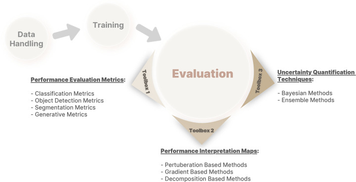
This report is the last in the Mitigating Bias in Radiology Machine Learning series (15,16) and focuses on potential bias during the performance evaluation of ML models. We first define the meaning of an appropriate fitness in ML, followed by a discussion of internal versus external testing of ML models. We then thoroughly discuss the three main toolboxes required for proper evaluation of model performance: (a) performance evaluation metrics, (b) performance interpretation maps, and (c) uncertainty quantification (UQ) techniques (Fig 1). Finally, we describe the appropriate application of techniques in each toolbox to avoid or minimize biases in ML model evaluation. Our primary goal is to address ML biases in radiology, but most of our discussion can be applied to other areas of ML in health care.

Figure 1:

A framework of different toolboxes in evaluation of deep learning model performance.

Determining “Fitness” in ML

After training an ML model, one must determine if the model fits properly to the data and if its fitness is affected by any biases. Model fitness can primarily be determined by observing the loss curves obtained during training, which is often the first step in evaluating a model's performance.

Model Underfitting

Training and validation loss curves may help identify two patterns that imply underfitting. The first pattern is characterized by a maintained downward slope of the validation loss curve during the entire training process, which implies that the model has not been trained fully and can be improved. Generally, model training should continue until the loss curve goes up for a sustained interval. The second pattern occurs when the training loss curve reaches a plateau instead of maintaining a downward slope, implying that the chosen model architecture may lack the required capacity (ie, has too few parameters) to sufficiently learn the problem at hand. Another, more frequent cause of underfitting is the presence of unoptimized hyperparameters, such as learning rate or the loss term, necessitating rigorous hyperparameter optimization and consideration of a more sophisticated model architecture. However, one may observe the same pattern of training loss if there is insufficient signal in the data to be learned by the model.

Model Overfitting

Detection of model overfitting can be more difficult. Traditionally, overfitting is defined as the point where the model's validation loss begins to increase while the training loss continues to decline. However, this is a naive approach for detecting overfitting, and relying on it can lead to inappropriate model selection. For example, diverging loss curves often happen transiently throughout the training process, such as when the learning rate is high (17). Another situation is training on highly imbalanced datasets. For instance, a model trained to detect a disease that has 1% prevalence may learn to always predict that the patient is healthy, resulting in a low validation loss value (if the loss is not weighted). As the model learns representative features, it might misclassify some healthy patients as those with disease, thus increasing validation loss values. However, this increased loss cannot be attributed to overfitting; instead, it implies that the model has started to learn a relevant set of features for classification, which are still imperfect. Therefore, loss curves cannot solely ensure correct training. Other tools, such as performance metrics, are needed to evaluate model performance. For example, increasing validation loss and F1 score would likely indicate that the model is learning through imperfect features that overlap between patients with and without disease.

Loss curves and metrics alone cannot guarantee a proper fit. There are instances when the metrics improve and the validation loss decreases, but the model fits on irrelevant information existing in the image. This occurs when the model selects features correlated with the desired outcome but not relevant to the desired application. For example, in a study for detecting femoral neck fractures from hip radiographs, a model could predict the outcome by learning the location where imaging took place (eg, the emergency department), the timing of imaging (eg, at night), and several other irrelevant features (18). This example emphasizes the need for inspecting the interpretation map of the model to determine if it is “focusing” on meaningful parts of the image.

Model fit can be determined by examining loss curves, metrics, and model interpretation maps. Different models with appropriate fitness levels can be trained on the same training data, where each shows superior performance in a set of metrics that are optimal for specific clinical scenarios. For example, in the case of creating a screening tool for a rare condition, a model with high sensitivity and negative predictive value is preferred over a model with high specificity. The performance evaluation metrics should be selected by clinical domain experts for a particular task.

Internal versus External Model Testing

Model testing can generally be categorized as “internal” or “external.” Internal testing uses the data from the same source as the training set that was held out during training, making the test data independent and identically distributed to the training data. There are different techniques to internally test an ML model, for example, simple train-validation-test split, cross-validation, and nested cross-validation (15). Although these techniques can help determine model fitness, internal testing may not detect biases present in the original data (19,20).

In contrast, external testing involves evaluating trained models on unseen external datasets with different populations (eg, race, age, sex, symptoms), enabling the detection and quantification of biases that may not be apparent using internal testing. Moreover, external testing helps to identify a recently described phenomenon called underspecification, which is the inability of a pipeline to identify whether a model has embedded the structure of the underlying system and will remain invariable in response to confounding factors (21). Larrazabal et al (22) showed that the performance of classifier models trained on the National Institutes of Health ChestX-Ray14 dataset differs significantly if applied to chest radiograph data from other sources. The underlying source of bias for these differences in model performance on external datasets was the sex distribution in the training dataset. As another example, a COVID-19 detection model trained on adults may be biased to adult presentations and less accurate in children (23). When these biases are detected, models can be retrained accordingly.

To properly perform external testing and avoid adding bias, researchers should first collect their external data from centers that are as similar as possible to the sites where their final model will be deployed. Second, datasets should include diverse populations (ie, age, sex, height, weight, body mass index, symptoms, etc) and conditions (ie, vendors, models, hardware, imaging protocols, etc) to assess the overall generalizability of the model. Finally, the preprocessing steps of external data should be identical to those of training data to ensure the external testing results remain fair and reliable. External testing based on an inappropriate dataset may underestimate model performance. For successful clinical use of a model, external testing must be incrementally performed and explained so clinicians comprehend the proper use cases and limitations of these models. The external testing process can be facilitated by open sourcing code, model weights, and, whenever possible, de-identified data to help reduce bias and make models more deployable.

In summary, external testing helps researchers understand how their models perform in real-world situations. Note that all tools reviewed in this report can be applied to internal and external test sets, as model performance should be compared on both types of test sets to fully understand the model and its underlying biases. Despite all its advantages, external testing is not always feasible due to difficulties in gaining access to proper external data. To address these issues, authors have recently suggested “stress testing” trained models as an alternative to external testing. This approach consists of obtaining a controlled shifted dataset from the original (internal) population and testing the trained model on this shifted dataset to identify its underspecifications (21,24).

Toolbox 1: Performance Evaluation Metrics

This section discusses commonly used performance metrics for various ML tasks, including their strengths and limitations and appropriate use to mitigate bias in performance evaluation.

Classification Tasks

Generally, classification tasks fall into three categories: binary (eg, to predict the presence or absence of pneumonia), multiclass (eg, distinguishing bacterial pneumonia, viral pneumonia, and no pneumonia), or multilabel (eg, looking for the presence or absence of pneumonia and the presence or absence of pneumothorax). We focus on binary classification metrics as they are easy to understand and can be extended to other classification types.

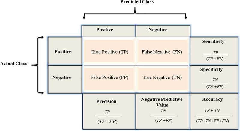
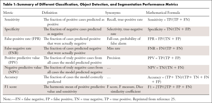
Confusion matrix.—Results of a binary classifier may be summarized in a confusion matrix (25) (Fig 2). Because each value represents one aspect of performance, looking at only one of them may lead to bias. For example, while seemingly optimal, a model with no false-negative findings may not be ideal if it produces many false-positive (FP) findings. To avoid bias in performance evaluation, one typically calculates metrics on the basis of combinations of confusion matrix values. Table 1 summarizes the definitions, formulas, and synonyms of these metrics (25).

Figure 2:

A confusion matrix and the associated calculations.

Table 1:

Summary of Different Classification, Object Detection, and Segmentation Performance Metrics

Which performance metrics to use to evaluate model performance depends highly on the clinical context of the problem (26,27). For example, if a model aims to screen breast cancer on mammograms, it is important to detect any suspicious lesions. Thus, a model with high sensitivity is preferred over a highly specific model. However, if we want to develop a model for confirming breast cancer, a more specific model would be more optimal. Moreover, there is often no specific threshold for performance metrics to determine if a model is performing well or not. For instance, identifying bacterial pneumonia using a chest radiograph with 80% sensitivity and 85% specificity may not appear impressive to thoracic radiologists, but the same metric values for identifying true progression versus pseudoprogression at MRI in patients with glioblastoma would be very valuable (28). To set a meaningful threshold for their metrics, developers need to review the previous literature and consult with clinicians to better understand what level of performance is required in clinical practice.

Accuracy.— Another consideration before selecting a set of performance metrics is how the strengths and limitations of each metric may impact the evaluation results (27). For instance, relying on the “accuracy” metric to evaluate model performance could lead to bias in the presence of severe data imbalance. Consider a model trained to detect glioblastoma in brain MRI studies that always predicts no brain tumor in each image. Such a model will have very high accuracy, as the incidence of glioblastoma is only 3.19 cases per 100 000 per year in the United States. Further, accuracy would be higher within an emergency department or oncology clinic. Instead of accuracy, a metric such as F1 score, receiver operating characteristic (ROC) curve, or precision-recall (PR) curve may better demonstrate model performance on imbalanced data (29). Nevertheless, accuracy remains a common metric because it is a single value and can be understood intuitively.

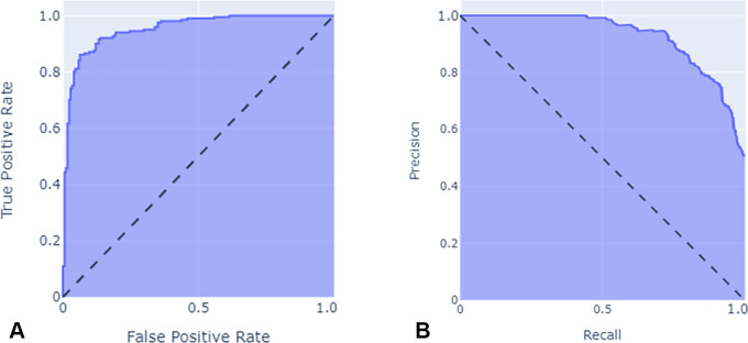
ROC and PR curves.— The ROC curve is a performance evaluation tool for balanced and imbalanced datasets that plots the true-positive (TP) rate (sensitivity) versus the FP rate (1 − specificity) at various threshold levels (30). In general, ROC curves that are closest to the left and top represent a better classifier, while a random guessing model would have a diagonal line from the bottom left of the plot to the top right, with an area under the ROC curve of 0.5 (Fig 3A).

Figure 3:

Illustration of (A) receiver operating characteristic curve and (B) precision-recall curve.

PR curves, an alternative to ROC curves, plot precision against recall at various thresholds. While there are some similarities between PR and ROC curves (30), the optimum threshold for each may differ, with the main difference being the importance of the true-negative rate. Imagine two models, A and B, that can detect the presence or absence on radiologic images of a particular tumor with a prevalence of 0.0001. Further, assume model A classifies 100 patients as tumor positive with 90 TPs in a collection of 1 000 000 images, while B classifies 2000 images as tumor positive with 90 TPs in the same collection. The TP rate and FP rate for models A versus B would be 0.9 and 0.00001 versus 0.9 and 0.00191, respectively. As presented here, the difference between FP rates is small (0.0019), but the precision and recall for models A versus B would be 0.9 and 0.9, versus 0.9 and 0.45, respectively; therefore, when there is a massive class imbalance, the area under the PR curve is more appropriate than the area under the ROC curve, as it more accurately summarizes a classifier's performance (31) (Fig 3B).

Segmentation

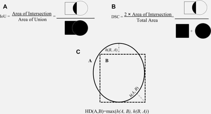
A segmentation model divides an image into different regions on the basis of the characteristics of pixels (voxels) to identify objects of interest (32). Segmentation models produce masks as outputs, in which nonzero pixel values correspond to the objects of interest in the original image, and pixels with zero values typically denote everything else (background). Segmentation models fall into two categories: semantic segmentation and instance segmentation, where the former assigns the same pixel value to multiple instances of the same object (eg, different lung nodules on a chest radiograph), and the latter labels them differently. While performance metrics are calculated based on the overall performance of a semantic segmentation model, instance-level metrics (ie, each structure being segmented) and the average of each across different instances are considered standard evaluation metrics. Many metrics are available to evaluate the performance of segmentation models, including accuracy, intersection over union (IoU), Dice similarity coefficient (DSC), and the Hausdorff distance (HD) (Fig 4). As different metrics can be sensitive to issues such as the presence of outliers (false-negative findings) or class imbalance, choosing the correct metric is critical to a fair evaluation of the model performance (33).

Figure 4:

Schematic illustration of segmentation performance metrics. Schematic definitions of (A) intersection over union (IoU), (B) Dice similarity coefficient (DSC), and (C) Hausdorff distance (HD).

Accuracy.—Although applicable, accuracy is rarely used to assess segmentation performance. Similar to classification tasks, accuracy tends to overestimate the performance of ML models in the presence of severe class imbalance, which is often the case, because the object is often small compared with background. For example, when an object of interest occupies 10% of the area in an image and the remaining pixels belong to the background, a model can achieve 90% accuracy on the segmentation task by predicting every pixel as background.

IoU.— The IoU measures the overlap between the predicted object contour and the ground truth contour (34) (Fig 4A). The IoU value ranges from 0 to 1, where 0 signifies no overlap, and 1 denotes complete overlap.

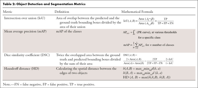
DSC.—DSC is a metric similar to IoU and is often used for semantic segmentation tasks, but it could also be used for object detection (35) (Fig 4B) (Table 2). Although DSC increases monotonically with respect to IoU, IoU penalizes incorrect classifications more severely than DSC. For example, suppose that most predictions from an object detection model, A, are moderately more accurate than those of another model, B, but some are substantially worse. DSC may favor model A in such a scenario, while IoU may be higher for model B (36).

Table 2:

Object Detection and Segmentation Metrics

HD.—Metrics like IoU or DSC are more often used to evaluate segmentation models, because they ignore the background and focus on the objects. However, these metrics do not consider the spatial distance between the model's predictions and the ground truth labels, an issue that can be mitigated using the HD.

Calculating the spatial distance between the edges of two objects is widely used in image segmentation to measure similarity. Considering the position of voxels, one may measure the distance between two contours. The HD between two finite point sets, A = {a₁,....,a_n} and B = {b₁,....,b_n}, is defined by HD (A, B) = max[h(A, B), h(B, A)], where h(A, B) and h(B, A) are called the directed HD and are calculated as shown in Equation (1) (Fig 4C),

Here, ∣d(a, b)∣ is the absolute value of Euclidean distance. To elaborate further, imagine the ground truth segmentation for an object of interest in an example image is A, and the predicted mask for that object is B. There is a distance σ that expands A such that A will completely cover B. Also, there is a distance γ that expands B such that it completely covers A. The maximum of the smallest possible σ for A and the smallest possible γ for B is defined as the HD. One challenge in using HD is its sensitivity to outliers (FPs), which could make HD meaningless (33,37,38). To mitigate this, researchers often use the 95th percentile of the average distance between two sets of points (sometimes known as HD₉₅).

The average HD (AHD) is defined as: AHD (A, B) = max [d_avg(A, B), d_avg(B, A)], where d_avg(A, B) and d_avg(B, A) are the AHD, and the distance between each point is calculated by the Euclidean distance (Eq 2).

In general, the AHD value ranges from 0 to higher positive numbers (depending on the units of the distance metric), with low AHD values considered optimal. Overall, similarity metrics (eg, DSC or IoU) or distance metrics (eg, Hausdorff or Mahalanobis) are useful metrics for evaluating segmentation models but may not be ideal for some tasks (39) and may require the use of multiple metrics simultaneously to interpret model performance.

Object Detection Tasks

An object detection model draws a rectangle (bounding box) around the object of interest and often begins by performing a regression task followed by a classification task. The regression task predicts bounding boxes to describe the spatial location of different objects of interest in an image, as opposed to segmentation, where the contour of the object of interest is precisely delineated. Each bounding box surrounds an object, specifies its location, and provides a box confidence score to show how likely it is that the box includes an object of interest (regardless of the class for that object). The classification task, on the other hand, uses these predicted bounding box regions to predict the object classes within them. The most common metrics used for object detection performance evaluation are IoU, mean average precision (mAP), and DSC.

To define mAP, we first need to define average precision (AP) and how it is affected by the IoU threshold. By setting an IoU threshold, one can label detections as correct or incorrect. With the presence of an object in a bounding box, any IoU value greater than or equal to the threshold value is considered as TP detection. Therefore, the confusion matrix for the classification performance of an object detection model depends on the IoU threshold set for that model. AP equals the area under the PR curve for a model detecting a specific class at various thresholds (Eq 3), with lower IoU thresholds resulting in higher AP scores. Averaging all the AP scores across all classes results in the mAP value (Eq 4). The higher the mAP score, the more accurate the model (40,41):

and

AP values may vary from very high for those classes with sufficient training data to very low for classes with fewer data. Therefore, the calculated mAP for a model does not reflect the model's performance for all classes. The mAP may be moderate if the model performs well for certain classes and poorly for others. In contrast, a high mAP value almost always indicates a consistently good performance across all classes and confidence levels.

Generative Models

Deep generative models (DGMs) are trained neural networks usually used to generate or improve images. While developing DGMs in computer vision has attracted increasing interest with applications such as superresolution, denoising, artifact reduction, and reconstruction, such applications are also important in clinical artificial intelligence tasks (42–45). DGMs generally transform acquired signals into images that are meaningful to humans and can be formulated as a multidimensional linear system,

in which x is the desired image based on the input image y. Ɛ is the encoder operator representing various generative tasks, for example, an identity operator for image denoising, image-space uniform undersampling for superresolution, local masking operators for in-painting, and k-space undersamples for MRI reconstruction. σ usually represents coherent noise by the measurement. In superresolution, for example, where x is the high-resolution image and y the corresponding low-resolution image, Ɛ represents an undersampling operation that turns x into y. The superresolution task tries to solve the inverse problem of Equation (5) to generate the original image x from y. However, the problem is indeterminate, as the solution x corresponding to y is not unique.

As a result, the generative task described by Equation (5) is ill-posed (46) and often reformulated as an optimization problem:

The resulting operation can therefore be solved by supervised learning.

Pixelwise metrics.—DGMs can generate high-quality images with properties needed for specific tasks. Thus, evaluating the generated image quality is critical for DGM applications in medical imaging.

Among the traditional metrics to evaluate the quality of generated images, mean-square error (MSE) is the most basic. It measures the average squared difference between pixels in two images:

Here, x and y are two images, and n is the number of pixels. The square root of MSE is also popular. Two other traditional metrics are peak signal-to-noise ratio (PSNR) and the structural similarity index measure (SSIM). PSNR is often used to measure the quality of digital signal transmission and is calculated as follows:

where max d is the maximum possible dynamic range of the image (usually 255 if an 8-bit image). On the other hand, SSIM is a perceptual quality metric and may better reflect what is seen than MSE and PSNR. The two-dimensional SSIM is formulated as:

where x̄ and ȳ are the averages of x and y pixel values, σ²_x and σ²_y are the variances of x and y, σ_xy is the covariance of x and y, and c₁ and c₂ are additional parameters. While MSE and PSNR are metrics in a pixelwise style, SSIM emphasizes the correlations between spatially nearby pixels, which may infer information regarding the higher-level image features.

It should be noted that all these metrics can be used as loss functions for training the DGM. In practice, PSNR and SSIM should be multiplied by -1 when doing so, as higher values indicate higher image quality.

Perceptual metrics.—One pitfall of using pixelwise metrics as a loss function is that although the trained model can achieve better validation metrics, it can also generate images that are too smooth, which may appear blurry compared with the ground truth high-resolution images. In practice, perceptual loss and generative adversarial networks loss are used to better capture the textural details and edges; thus, perceptual quality metrics such as perceptual index and natural image quality evaluator are also proposed in the literature for evaluating generative models (47,48). Therefore, researchers often use a combination of pixelwise and perceptual quality metrics to evaluate generative model performance. Almost all these image quality measures rely on the ground truth image, and whether they should be used alone or in combination with other metrics depends on the generative task at hand.

Compared with physics-informed deep learning models (eg, compressed sensing), generative adversarial networks may create fake findings in an image because of instability in training and pseudorealistic output. Thus, blind evaluation by radiologists is highly recommended when evaluating the textural and diagnostic qualities of clinical images generated by ML models compared with real medical imaging.

Toolbox 2: Performance Interpretation Maps

We described several metrics that are frequently used to evaluate the performance of ML models. However, relying on such metrics alone cannot guarantee that a model is free of bias, even in the presence of acceptable metric values, as models may have accidentally fit to meaningless noise in the input data. Deep evaluation of an ML model performance, therefore, also depends on interpreting the decision-making process of ML models.

Performance interpretation maps show where a trained neural network “looks” at an image in a computer vision task. It allows one to identify what the model considers discriminative parts of an image. Thus, an interpretation map may help diagnose failure modes and detect bias in computer vision tasks. Post hoc interpretation maps, in general, create heatmaps to describe how different parts of an image influence the model's decision on a pixel-by-pixel basis (49,50). In a well-trained model, class-specific features outweigh other features. In contrast, a biased model detects incorrect features rather than the meaningful signal in the images. With all these considerations in mind, a good interpretation map helps answer the following questions: How does the model use the input data to fulfill its purpose? Where are the features most responsible for the output? Does the model capture relevant relationships within the data (51)?

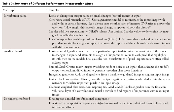
Currently available post hoc interpretation maps generally fall into three categories: perturbation-based approaches, backpropagation-based or gradient-based approaches, and decomposition-based approaches. As an alternative to post hoc attribution, trainable attention modules can be attached to typical convolutional neural network architectures to produce so-called attention maps during model training (50). Table 3 summarizes available methods and provides examples.

Table 3:

Summary of Different Performance Interpretation Maps

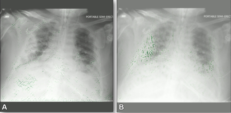
Despite these potential benefits of interpretation maps (Fig 5), they do have important limitations. Most notably, there is concern that explanations derived from attribution-based interpretation methods, such as saliency mapping or class activation maps, are unreliable and misleading (52,53). For instance, Seah et al (54) reported that heatmaps on frontal chest radiographs did not represent the expected abnormality of heart failure after using several attribution-based interpretation methods (occlusions, integrated gradients, and local interpretable model-agnostic explanations). However, the expected abnormalities (cardiomegaly and low body mass) could be visualized using generative visual rationale. Additionally, Böhle et al (55) found that guided backpropagation did not produce interpretation maps that were visually distinguishable in Alzheimer disease versus healthy controls using T1-weighted brain MRI studies. In a recent study, Arun et al (56) assessed interpretation maps using four critical trustworthiness criteria: utility, sensitivity to weight randomization, repeatability (intra-architecture), and reproducibility (interarchitecture). The authors concluded that saliency maps should be scrutinized more closely in the high-risk domain of diagnostic medical imaging and recommended using detection or segmentation models instead of saliency maps if localization is desired. In summary, interpretation maps can be used to identify biases, but researchers should consider their limitations.

Figure 5:

Example gradient-weighted class activation mapping images for two COVID-19 detection models. Both models have the same level of accuracy on the same test data. (A) Image shows a biased model localizing the incorrect part of the chest radiograph as the opacity. (B) Image shows a properly trained model localizing the correct part of the chest radiograph. Green dots represent localization.

Toolbox 3: UQ Techniques

UQ techniques measure the confidence of a model, depicting the trustworthiness of its predictions. Moreover, UQ can demonstrate the biases resulting in overconfidence or underconfidence in model predictions. UQ identifies when medical ML models have insufficient information to make a reliable decision, thus informing users that an output has low trust. In this way, the model communicates with medical experts and likely increases trust in model performance over time (57,58).

Uncertainty can be divided into two categories: aleatoric and epistemic. Aleatoric uncertainty (data uncertainty) is noise in the data and thus is irreducible regardless of how we train the model. In contrast, epistemic uncertainty (knowledge uncertainty) is the less-than-perfect model performance that can be lessened by gathering enough training data and improving the model over time. Usually, model uncertainty refers to epistemic uncertainty, which is focused on here (59,60).

Performing UQ can be a challenging task for developers and may lead to bias if done improperly. When performing UQ, developers should pay attention to the calibrated confidence of a model in addition to its predictions. The calibrated confidence of a model indicates how close the predicted model output values are to the real probability of those outcomes. For example, suppose a chest radiograph classifier that ends with a softmax function predicts values of 0.1, 0.2, and 0.7 for three output classes of normal, viral pneumonia, or bacterial pneumonia, respectively. This model's confidence could be considered calibrated if the real-world probability of the patient having viral pneumonia is close to 0.2. However, previous research has shown that models ending with softmax layers are prone to low calibration; therefore, softmax output is not an acceptable approach for assessing the trustworthiness of a model, especially in the medical field (61–63).

Although there are many UQ techniques in ML research, the more popular techniques may be classified into three groups (64,65):

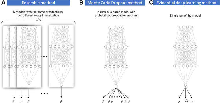
1. Bayesian methods approximate the posterior distributions of model weights (parameters) and capture how much these weights vary over the data, either during training or inference. A famous Bayesian method is Monte Carlo dropout, in which different instances of a single model are formed by randomly changing the level of contribution of different nodes in each instance during inference (similar to dropout regularization). Comparing the performance of each model instance with a different configuration yields a distribution of the model's predictions, which helps estimate the model's level of uncertainty (61).

2. Ensemble methods require training many instances of the same model on the same training data but with different random seeds. All predictions made by each model instance are ensembled to form a final prediction (typically the average of all instances). The uncertainty measure is based on the variance of the individual predictions (66).

3. Evidential deep learning methods treat learning as an evidence acquisition process. These methods represent a model's predictions as an evidential distribution of possible outputs, not a point estimate of a single output. The model is then trained to find the hyperparameters of the evidential distribution. Dirichlet and inverse-gamma distributions are examples of such evidential distributions that have been proposed for predictions from classification and regression models, respectively (67–69).

Evidential deep learning methods have two advantages over Bayesian and ensemble methods: (a) Applying them is less computationally costly, as there is no need to run multiple instances of a model during training or inference; and (b) they can both quantify model uncertainty and calibrate the model during training. Regarding the latter point, it should be noted that not all UQ methods can calibrate ML models. Likewise, not all methods for model calibration are capable of UQ, such as label smoothing (70) (Fig 6).

Figure 6:

A schematic illustration of different uncertainty quantification methods. (A) Ensemble method by training k models with the same architectures but different weight initialization. (B) Monte Carlo dropout method by running the same model k times with probabilistic dropout for each run. (C) Evidential deep learning (EDL) method by training the model with EDL loss function.

All these techniques can provide researchers with measures such as the confidence interval for model predictions and can ultimately help evaluate model uncertainty.

Conclusion

This report summarizes the main concepts, techniques, and caveats in evaluating ML model performance. We reviewed the concept of fit and how loss function outputs can demonstrate underfitting or overfitting. We then contrasted internal and external evaluation and highlighted why external testing is superior to internal testing in bias detection. Finally, we discussed three main toolboxes and their most frequently used techniques that researchers can use to detect biases in model performance: performance evaluation metrics, performance interpretation maps, and UQ techniques. In conclusion, evaluating model performance is not a straightforward path of several steps; instead, it is a highly task-dependent process that could quickly become complicated. One should be mindful that evaluation of model performance is an effort to answer critical questions regarding model preparedness to be deployed in its target clinical settings. Therefore, it is crucial to include domain experts when selecting and interpreting the results of model performance evaluation.

References

- 1. Yang X , Wang Y , Byrne R , Schneider G , Yang S . Concepts of artificial intelligence for computer-assisted drug discovery . Chem Rev 2019. ; 119 ( 18 ): 10520 – 10594 . [DOI] [PubMed] [Google Scholar]
- 2. Burton RJ , Albur M , Eberl M , Cuff SM . Using artificial intelligence to reduce diagnostic workload without compromising detection of urinary tract infections . BMC Med Inform Decis Mak 2019. ; 19 ( 1 ): 171 . [DOI] [PMC free article] [PubMed] [Google Scholar]
- 3. Cho BJ , Choi YJ , Lee MJ , et al . Classification of cervical neoplasms on colposcopic photography using deep learning . Sci Rep 2020. ; 10 ( 1 ): 13652 . [DOI] [PMC free article] [PubMed] [Google Scholar]
- 4. Wiens J , Saria S , Sendak M , et al . Do no harm: a roadmap for responsible machine learning for health care . Nat Med 2019. ; 25 ( 9 ): 1337 – 1340 . [Published correction appears in Nat Med 2019;25(10):1627.] [DOI] [PubMed] [Google Scholar]
- 5. Char DS , Shah NH , Magnus D . Implementing machine learning in health care - addressing ethical challenges . N Engl J Med 2018. ; 378 ( 11 ): 981 – 983 . [DOI] [PMC free article] [PubMed] [Google Scholar]
- 6. Obermeyer Z , Powers B , Vogeli C , Mullainathan S . Dissecting racial bias in an algorithm used to manage the health of populations . Science 2019. ; 366 ( 6464 ): 447 – 453 . [DOI] [PubMed] [Google Scholar]
- 7. Chen IY , Joshi S , Ghassemi M . Treating health disparities with artificial intelligence . Nat Med 2020. ; 26 ( 1 ): 16 – 17 . [DOI] [PubMed] [Google Scholar]
- 8. Shortliffe EH , Sepúlveda MJ . Clinical decision support in the era of artificial intelligence . JAMA 2018. ; 320 ( 21 ): 2199 – 2200 . [DOI] [PubMed] [Google Scholar]
- 9. Li X , Xiong H , Li X , et al . Interpretable Deep Learning: Interpretation, Interpretability, Trustworthiness, and Beyond . arXiv:2103.10689 [preprint] https://arxiv.org/abs/2103.10689. Posted March 19, 2021 .
- 10. Caruana R , Lou Y , Gehrke J , Koch P , Sturm M , Elhadad N . intelligible models for healthcare: predicting pneumonia risk and hospital 30-day readmission . In : Proceedings of the 21th ACM SIGKDD International Conference on Knowledge Discovery and Data Mining . New York, NY : Association for Computing Machinery ; 2015. ; 1721 – 1730 . [Google Scholar]
- 11. Holzinger A , Biemann C , Pattichis CS , Kell DB . What do we need to build explainable AI systems for the medical domain? arXiv:1712.09923 [preprint] https://arxiv.org/abs/1712.09923. Posted December 28, 2017 .
- 12. Ahmad MA , Eckert C , Teredesai A . Interpretable Machine Learning in Healthcare . In : Proceedings of the 2018 ACM International Conference on Bioinformatics, Computational Biology, and Health Informatics . New York, NY : Association for Computing Machinery ; 2018. ; 559 – 560 . [Google Scholar]
- 13. Mcknight DH , Carter M , Thatcher JB , Clay PF . Trust in a specific technology: An investigation of its components and measures . ACM Trans Manage Inf Syst 2011. ; 2 ( 2 ): 1 – 25 . [Google Scholar]
- 14. Juravle G , Boudouraki A , Terziyska M , Rezlescu C . Trust in artificial intelligence for medical diagnoses . Prog Brain Res 2020. ; 253 : 263 – 282 . [DOI] [PubMed] [Google Scholar]
- 15. Rouzrokh P , Khosravi B , Faghani S , et al . Mitigating Bias in Radiology Machine Learning: 1. Data Handling . Radiol Artif Intell 2022. ; 4 ( 5 ): e210290 . [DOI] [PMC free article] [PubMed] [Google Scholar]
- 16. Zhang K , Khosravi B , Vahdati S , et al . Mitigating Bias in Radiology Machine Learning: 2. Model Development . Radiol Artif Intell 2022. ; 4 ( 5 ): e220010 . [DOI] [PMC free article] [PubMed] [Google Scholar]
- 17. Smith LN . A disciplined approach to neural network hyper-parameters: Part 1 – learning rate, batch size, momentum, and weight decay . arXiv:1803.09820 [preprint] https://arxiv.org/abs/1803.09820 Posted March 26, 2018 .
- 18. Badgeley MA , Zech JR , Oakden-Rayner L , et al . Deep learning predicts hip fracture using confounding patient and healthcare variables . NPJ Digit Med 2019. ; 2 ( 1 ): 31 . [DOI] [PMC free article] [PubMed] [Google Scholar]
- 19. Ho SY , Phua K , Wong L , Bin Goh WW . Extensions of the external validation for checking learned model interpretability and generalizability . Patterns (N Y) 2020. ; 1 ( 8 ): 100129 . [DOI] [PMC free article] [PubMed] [Google Scholar]
- 20. Park SH , Han K . Methodologic guide for evaluating clinical performance and effect of artificial intelligence technology for medical diagnosis and prediction . Radiology 2018. ; 286 ( 3 ): 800 – 809 . [DOI] [PubMed] [Google Scholar]
- 21. Eche T , Schwartz LH , Mokrane FZ , Dercle L . Toward generalizability in the deployment of artificial intelligence in radiology: role of computation stress testing to overcome underspecification . Radiol Artif Intell 2021. ; 3 ( 6 ): e210097 . [DOI] [PMC free article] [PubMed] [Google Scholar]
- 22. Larrazabal AJ , Nieto N , Peterson V , Milone DH , Ferrante E . Gender imbalance in medical imaging datasets produces biased classifiers for computer-aided diagnosis . Proc Natl Acad Sci U S A 2020. ; 117 ( 23 ): 12592 – 12594 . [DOI] [PMC free article] [PubMed] [Google Scholar]
- 23. Chen A , Huang JX , Liao Y , et al . Differences in clinical and imaging presentation of pediatric patients with COVID-19 in comparison with adults . Radiol Cardiothorac Imaging 2020. ; 2 ( 2 ): e200117 . [DOI] [PMC free article] [PubMed] [Google Scholar]
- 24. D'Amour A , Heller K , Moldovan D , et al . Underspecification presents challenges for credibility in modern machine learning . arXiv:2011.03395 [preprint] https://arxiv.org/abs/2011.03395 Posted November 6, 2020 . [Google Scholar]
- 25. Erickson BJ , Kitamura F . Magician's Corner: 9. Performance metrics for machine learning models . Radiol Artif Intell 2021. ; 3 ( 3 ): e200126 . [DOI] [PMC free article] [PubMed] [Google Scholar]
- 26. Reinke A , Tizabi MD , Sudre CH , et al . Common limitations of image processing metrics: a picture story . arXiv:2104.05642 [preprint] https://arxiv.org/abs/2104.05642. Posted April 12, 2021 . [Google Scholar]
- 27. Maier-Hein L , Reinke A , Christodoulou E , et al . Metrics reloaded: Pitfalls and recommendations for image analysis validation . arXiv:2206.01653 [preprint] https://arxiv.org/abs/2206.01653. Posted June 3, 2022 . [Google Scholar]
- 28. Moassefi M , Faghani S , Conte GM , et al . A deep learning model for discriminating true progression from pseudoprogression in glioblastoma patients . J Neurooncol 2022. . 10.1007/s11060-022-04080-x. Published online July 19, 2022 . [DOI] [PubMed] [Google Scholar]
- 29. Tamimi AF , Juweid M . Epidemiology and outcome of glioblastoma . In : De Vleeschouwer S , ed. Glioblastoma . Brisbane, Australia: : Codon Publications; , 2017. . [PubMed] [Google Scholar]
- 30. Sokolova M , Japkowicz N , Szpakowicz S . Beyond accuracy, F-Score and ROC: A family of discriminant measures for performance evaluation . In : Sattar A , Kang Bh , eds. AI 2006: Advances in Artificial Intelligence. AI 2006. Lecture Notes in Computer Science , vol 4304 . Berlin, Germany: : Springer; , 2006. ; 1015 – 1021 . [Google Scholar]
- 31. Ozenne B , Subtil F , Maucort-Boulch D . The precision--recall curve overcame the optimism of the receiver operating characteristic curve in rare diseases . J Clin Epidemiol 2015. ; 68 ( 8 ): 855 – 859 . [DOI] [PubMed] [Google Scholar]
- 32. Zaitoun NM , Aqel MJ . Survey on image segmentation techniques . Procedia Comput Sci 2015. ; 65 : 797 – 806 . [Google Scholar]
- 33. Taha AA , Hanbury A . Metrics for evaluating 3D medical image segmentation: analysis, selection, and tool . BMC Med Imaging 2015. ; 15 ( 1 ): 29 . [DOI] [PMC free article] [PubMed] [Google Scholar]
- 34. Rezatofighi H , Tsoi N , Gwak J , Sadeghian A , Reid I , Savarese S . Generalized intersection over union: a metric and a loss for bounding box regression . In : 2019 IEEE/CVF Conference on Computer Vision and Pattern Recognition (CVPR) . Piscataway, NJ: : IEEE; ; 2019. ; 658 – 666 . [Google Scholar]
- 35. Bertels J , Eelbode T , Berman M , et al . Optimizing the Dice score and Jaccard index for medical image segmentation: theory & practice . arXiv:1911.01685 [preprint] https://arxiv.org/abs/1911.01685 Posted November 5, 2019 . [Google Scholar]
- 36. Eelbode T , Bertels J , Berman M , et al . Optimization for medical image segmentation: theory and practice when evaluating with Dice score or Jaccard index . IEEE Trans Med Imaging 2020. ; 39 ( 11 ): 3679 – 3690 . [DOI] [PubMed] [Google Scholar]
- 37. Gerig G , Jomier M , Chakos M . Valmet: A new validation tool for assessing and improving 3D object segmentation . In : Niessen WJ , Viergever MA , eds. Medical Image Computing and Computer-Assisted Intervention – MICCAI 2001. MICCAI 2001. Lecture Notes in Computer Science , vol 2208 . Berlin, Germany: : Springer; , 2001. ; 516 – 523 . [Google Scholar]
- 38. Zhang D , Lu G . Review of shape representation and description techniques . Pattern Recognit 2004. ; 37 ( 1 ): 1 – 19 . [Google Scholar]
- 39. De Maesschalck R , Jouan-Rimbaud D , Massart DL . The Mahalanobis distance . Chemom Intell Lab Syst 2000. ; 50 ( 1 ): 1 – 18 . [Google Scholar]
- 40. Redmon J , Farhadi A . YOLOv3: An incremental improvement . arXiv:1804.02767 [preprint] https://arxiv.org/abs/1804.02767. Posted April 8, 2018. Accessed November 30, 2021 . [Google Scholar]
- 41. Szegedy C , Toshev A , Erhan D . Deep neural networks for object detection . https://proceedings.neurips.cc/paper/2013/hash/f7cade80b7cc92b991cf4d2806d6bd78-Abstract.html. Published 2013 . [Google Scholar]
- 42. Li Z , Zhou S , Huang J , Yu L , Jin M . Investigation of Low-Dose CT Image Denoising Using Unpaired Deep Learning Methods . IEEE Trans Radiat Plasma Med Sci 2021. ; 5 ( 2 ): 224 – 234 . [DOI] [PMC free article] [PubMed] [Google Scholar]
- 43. Zhang K , Hu H , Philbrick K , et al . SOUP-GAN: Super-Resolution MRI Using Generative Adversarial Networks . arXiv:2106.02599 [preprint] https://arxiv.org/abs/2106.02599. Posted June 4, 2021 . [DOI] [PMC free article] [PubMed] [Google Scholar]
- 44. Liu G , Cao Z , Xu Q , et al . Recycling diagnostic MRI for empowering brain morphometric research - Critical & practical assessment on learning-based image super-resolution . Neuroimage 2021. ; 245 : 118687 . [DOI] [PubMed] [Google Scholar]
- 45. Hammernik K , Klatzer T , Kobler E , et al . Learning a variational network for reconstruction of accelerated MRI data . Magn Reson Med 2018. ; 79 ( 6 ): 3055 – 3071 . [DOI] [PMC free article] [PubMed] [Google Scholar]
- 46. Benning M , Burger M . Modern regularization methods for inverse problems . Acta Numer 2018. ; 27 : 1 – 111 . [Google Scholar]
- 47. Johnson J , Alahi A , Li FF . Perceptual losses for real-time style transfer and super-resolution . In : Leibe B , Matas J , Sebe N , Welling M , eds. Computer Vision – ECCV 2016. ECCV 2016. Lecture Notes in Computer Science , vol 9906 . Cham: Switzerland: : Springer; , 2016. ; 694 – 711 . [Google Scholar]
- 48. Blau Y , Mechrez R , Timofte R , Michaeli T , Zelnik-Manor L . The 2018 PIRM Challenge on Perceptual Image Super-resolution . arXiv preprint arXiv:1809.07517. https://arxiv.org/abs/1809.07517. Posted September 20, 2018 . [Google Scholar]
- 49. Ribeiro MT , Singh S , Guestrin C . “Why should I trust you?”: Explaining the predictions of any classifier . In : Proceedings of the 22nd ACM SIGKDD International Conference on Knowledge Discovery and Data Mining . New York, NY : Association for Computing Machinery ; 2016. ; 1135 – 1144 . [Google Scholar]
- 50. Huff DT , Weisman AJ , Jeraj R . Interpretation and visualization techniques for deep learning models in medical imaging . Phys Med Biol 2021. ; 66 ( 4 ): 04TR01 . [DOI] [PMC free article] [PubMed] [Google Scholar]
- 51. Pereira S , Meier R , McKinley R , et al . Enhancing interpretability of automatically extracted machine learning features: application to a RBM-Random Forest system on brain lesion segmentation . Med Image Anal 2018. ; 44 : 228 – 244 . [DOI] [PubMed] [Google Scholar]
- 52. Adebayo J , Gilmer J , Muelly M , Goodfellow I , Hardt M , Kim B . Sanity checks for saliency maps . arXiv:1810.03292 [preprint] https://arxiv.org/abs/1810.03292. Posted October 8, 2018 . [Google Scholar]
- 53. Rudin C . Stop Explaining Black Box Machine Learning Models for High Stakes Decisions and Use Interpretable Models Instead . arXiv:1811.10154 [preprint] https://arxiv.org/abs/1811.10154. Posted November 26, 2018 . [DOI] [PMC free article] [PubMed]
- 54. Seah JCY , Tang JSN , Kitchen A , Gaillard F , Dixon AF . Chest radiographs in congestive heart failure: visualizing neural network learning . Radiology 2019. ; 290 ( 2 ): 514 – 522 . [DOI] [PubMed] [Google Scholar]
- 55. Böhle M , Eitel F , Weygandt M , Ritter K . Layer-wise relevance propagation for explaining deep neural network decisions in MRI-based Alzheimer's disease classification . Front Aging Neurosci 2019. ; 11 : 194 . [DOI] [PMC free article] [PubMed] [Google Scholar]
- 56. Arun N , Gaw N , Singh P , et al . Assessing the trustworthiness of saliency maps for localizing abnormalities in medical imaging . Radiol Artif Intell 2021. ; 3 ( 6 ): e200267 . [DOI] [PMC free article] [PubMed] [Google Scholar]
- 57. Begoli E , Bhattacharya T , Kusnezov D . The need for uncertainty quantification in machine-assisted medical decision making . Nat Mach Intell 2019. ; 1 ( 1 ): 20 – 23 . [Google Scholar]
- 58. Kompa B , Snoek J , Beam AL . Second opinion needed: communicating uncertainty in medical machine learning . NPJ Digit Med 2021. ; 4 ( 1 ): 4 . [DOI] [PMC free article] [PubMed] [Google Scholar]
- 59. Kiureghian AD , Ditlevsen O . Aleatory or epistemic? Does it matter? Struct Saf 2009. ; 31 ( 2 ): 105 – 112 . [Google Scholar]
- 60. Kendall A , Gal Y . What uncertainties do we need in Bayesian deep learning for computer vision? arXiv:1703.04977 [preprint] https://arxiv.org/abs/1703.04977. Posted March 15, 2017 . [Google Scholar]
- 61. Gal Y , Ghahramani Z . Dropout as a Bayesian approximation: representing model uncertainty in deep learning . In : Balcan MF , Weinberger KQ , eds. Proceedings of the 33rd International Conference on Machine Learning , June 20–22, 2016 . New York, NY: : PMLR; , 2016. ; 1050 – 1059 . [Google Scholar]
- 62. Guo C , Pleiss G , Sun Y , Weinberger KQ . On calibration of modern neural networks . In : Precup D , Teh YW , eds. Proceedings of the 34th International Conference on Machine Learning. PMLR , 2017. ; 1321 – 1330 . [Google Scholar]
- 63. Benchmarking uncertainty estimation methods for deep learning with safety-related metrics . http://publica.fraunhofer.de/dokumente/N-582723.html. Accessed February 13, 2022 .
- 64. Abdar M , Pourpanah F , Hussain S , et al . A review of uncertainty quantification in deep learning: Techniques, applications and challenges . Inf Fusion 2021. ; 76 : 243 – 297 . [Google Scholar]
- 65. Caldeira J . Deeply uncertain: Comparing methods of uncertainty quantification in deep learning algorithms [slides] . Fermi National Accelerator Laboratory (FNAL) . Published April 15, 2020.
- 66. Lakshminarayanan B , Pritzel A , Blundell C . Simple and scalable predictive uncertainty estimation using deep ensembles . arXiv:1612.01474 [preprint] https://arxiv.org/abs/1612.01474. Posted December 5, 2016 . [Google Scholar]
- 67. Amini A , Schwarting W , Soleimany A , Rus D . Deep evidential regression . arXiv:1910.02600 [preprint] https://arxiv.org/abs/1910.02600. Posted October 7, 2019 . [Google Scholar]
- 68. Sensoy M , Kaplan L , Kandemir M . Evidential deep learning to quantify classification uncertainty . arXiv:1806.01768 [preprint] https://arxiv.org/abs/1806.01768. Posted June 5, 2018 . [Google Scholar]
- 69. Khosravi B , Faghani S , Ashraf-Ganjouei A . Uncertainty quantification in COVID-19 detection using evidential deep learning . medRxiv:2022.05.29.22275732 [preprint] https://www.medrxiv.org/content/10.1101/2022.05.29.22275732v1. Posted May 29, 2022 . [Google Scholar]
- 70. Müller R , Kornblith S , Hinton G . When Does Label Smoothing Help? arXiv:1906.02629 [preprint] https://arxiv.org/abs/1906.02629. Posted June 6, 2019 . [Google Scholar]