Abstract
High‐resolution space‐based spectral imaging of the Earth's surface delivers critical information for monitoring changes in the Earth system as well as resource management and utilization. Orbiting spectrometers are built according to multiple design parameters, including ground sampling distance (GSD), spectral resolution, temporal resolution, and signal‐to‐noise ratio. Different applications drive divergent instrument designs, so optimization for wide‐reaching missions is complex. The Surface Biology and Geology component of NASA's Earth System Observatory addresses science questions and meets applications needs across diverse fields, including terrestrial and aquatic ecosystems, natural disasters, and the cryosphere. The algorithms required to generate the geophysical variables from the observed spectral imagery each have their own inherent dependencies and sensitivities, and weighting these objectively is challenging. Here, we introduce intrinsic dimensionality (ID), a measure of information content, as an applications‐agnostic, data‐driven metric to quantify performance sensitivity to various design parameters. ID is computed through the analysis of the eigenvalues of the image covariance matrix, and can be thought of as the number of significant principal components. This metric is extremely powerful for quantifying the information content in high‐dimensional data, such as spectrally resolved radiances and their changes over space and time. We find that the ID decreases for coarser GSD, decreased spectral resolution and range, less frequent acquisitions, and lower signal‐to‐noise levels. This decrease in information content has implications for all derived products. ID is simple to compute, providing a single quantitative standard to evaluate combinations of design parameters, irrespective of higher‐level algorithms, products, applications, or disciplines.
Keywords: intrinsic dimensionality, mission design, hyperspectral, imaging spectroscopy, surface biology and geology
Key Points
Intrinsic dimensionality (ID) is the size of the signal subspace, or the number of significant principal components in a hyperspectral image
ID is an applications‐agnostic metric that can evaluate imaging spectroscopy instrument and mission design
Spatial, spectral, temporal resolution, and noise directly impact ID for a wide range of Earth surface scenes
1. Introduction
The ability to accurately measure and forecast the Earth system is increasingly important as climate change drives transformation across all scales (IPCC, 2021). In the last decade, various remote sensing satellite instruments have increased the range, scale, and impact of Earth observations, leading to important breakthroughs across Earth Science. The National Aeronautics and Space Administration (NASA) launched the Gravity Recovery and Climate Experiment (GRACE) missions to provide valuable data on water storage and glacier wasting (Landerer et al., 2020; Landerer & Swenson, 2012; Schmidt et al., 2006). The European Space Agency (ESA) designed the Soil Moisture and Ocean Salinity mission to understand two important parts of the water cycle (Jackson et al., 2011; Kerr et al., 2001). The Orbiting Carbon Observatory missions improve our understanding of the global carbon cycle (Crisp et al., 2004; Eldering et al., 2017), and the ECOsystem Spaceborne Thermal Radiometer Experiment on Space Station (ECOSTRESS) provides critical metrics on plant heat stress and water uptake (Fisher et al., 2020; Pascolini‐Campbell et al., 2021; Xiao et al., 2021). These missions were each optimized to measure a specific quantity or for a particular application that dictated all hardware and mission design decisions. In contrast, the next generation of NASA missions will be increasingly interdisciplinary, delivering a variety of measurements that touch on many science topics and aspects of the Earth System. For example, the NISAR mission will deliver products related to water availability, geologic hazards, and ecosystem biomass. Such missions cannot be traced to a single measurement objective, and when discipline requirements conflict, it is not clear how to make design decisions with finite mission resources. A consistent metric is necessary to understand the data needs and applications across diverse ecosystems.
As an example of how discipline needs may conflict with each other, consider the problem of orbit selection. A geostationary orbit provides the opportunity to continuously monitor ∼30% of the Earth's surface in its field of view, but the ∼30,000 km orbit altitude and constraints on optics size and mass effectively limits GSD; for example, the latest GOES satellites have 500 m GSD in the visible, 1 km GSD in the near‐infrared, and 2 km GSD in the thermal infrared (TIR). Polar‐orbiting satellites acquire data at fine spatial scales (5–30 m) less frequently (5–16 days revisit). Thus, there is a trade‐off between spatial and temporal resolution, and these dynamics compete with challenges in available instrument technology. Determining the optimal satellite revisit and resolution is often dependent on the application. There are also interlinked relationships between spectral resolution and spectral range, spatial resolution and swath width, radiometric resolution and saturation, and many other considerations that need to be optimized. Better integration of this great diversity of measurements would benefit the state of the science.
We address this problem through the lens of intrinsic dimensionality (ID), a universal performance metric, and its implications for an important new NASA mission: the Surface Biology and Geology (SBG) investigation. SBG will employ high GSD hyperspectral visible to shortwave infrared (VSWIR) and multi‐spectral TIR imagery to meet diverse science and applications needs (Stavros et al., 2022). In theory, each of these observations is constrained by its own set of high‐priority parameters (Cawse‐Nicholson et al., 2021). For instance, geologists might be more interested in high spectral resolution than frequent revisit (Swayze et al., 2003). Aquatic scientists might be more interested in minimal instrument noise over dark targets than <100 m GSD (Dierssen et al., 2021), and volcanologists might prioritize revisit frequency (Francis & Rothery, 2000). As the measurement science advances, instruments are also drafted into roles beyond their original design purpose, such as the use of airborne VSWIR instruments to monitor greenhouse gas point sources (Duren et al., 2019). Rather than trying to arbitrate between all possible measurement objectives—an impossible and ever evolving task—we propose an alternative standard of instrument performance related to the information captured from the upwelling light field. Specifically, we show how the ID, which quantifies the number of measurable free parameters in a data set, is a reasonable and objective standard of SBG observing system performance that broadly captures diverse science and application needs.
2. Intrinsic Dimensionality
ID is a measure of information content that has been used to determine components of chemical mixtures from hyperspectral data (Kritchman & Nadler, 2008), retrieve speech signals from noisy audio (Park et al., 1999), measure the impact of data fusion (Cawse‐Nicholson et al., 2019), and determine unique classes in remotely sensed imagery (Asner et al., 2012; Boardman & Green, 2000; Small, 2001; Thompson et al., 2017). ID quantifies the number of significant principal components. If a hyperspectral image , of size , where is the number of pixels and is the number of spectral bands, can be written as a linear combination of signal () and noise (), such that , then the ID is the rank of the signal subspace (i.e., the maximum number of linearly independent components when noise is disregarded).
We assume that each pixel can be written as a linear combination of endmembers (objects contained within the scene with unique spectral properties), such that:
| (1) |
where is the noise present in the ith pixel, is the abundance of the jth endmember in the ith pixel, and is the ID. Here, the noise encapsulates all causes of uncertainty that might cause a deviation from the true radiance, including photon shot noise, electronic noise, read noise, dark current noise, quantization noise, and other calibration uncertainties. If the endmembers are known (from field measurements or an existing spectral library), then the abundances can be determined using fully constrained least squares (C.‐I. Chang & Heinz, 2000) or other optimization techniques. To be meaningful, , and . If the endmembers are not known, as is often the case, can be estimated from the image if is known, using simplex algorithms or other techniques. Simplex algorithms assume that all mixed pixel vectors can be enclosed by a K‐dimensional simplex, where the simplex endpoints are the vectors representing pure spectra (e.g., C.‐I. Chang et al., 2006; Nascimento & Bioucas Dias, 2005; Winter, 1999).
In natural ecosystems, there is some inherent variability within classes, representing for example, different nutrient levels within trees of the same species. In such cases, the endmember can be thought of as the center or most representative spectrum from a class, and highly variable species may be represented by multiple classes. Natural variation is distinguished from noise by the assumption that naturally varying spectra within a class will, for the most part, change smoothly across the electromagnetic spectrum, whereas the noise is random between spectral channels.
Several methods have been proposed to estimate in Equation 1, which is the ID (e.g., Bachmann et al., 2008; Berman, 2019; Bioucas‐Dias & Nascimento, 2005; Cawse‐Nicholson et al., 2012; C.‐I. Chang & Du, 2004). We use random matrix theory (RMT) to estimate ID (Cawse‐Nicholson et al., 2012, 2019). If the noise is assumed to be Gaussian, we can construct a “random matrix” , where each column of is a random vector that has been drawn from a Gaussian distribution. The eigenvalues of these random matrices have been studied (Baik & Silverstein, 2006; Johnstone, 2001). While it is possible that there are non‐Gaussian contributors to the noise term in Equation 1, the Gaussian assumption is common and has been shown to be sufficient in practice (Bioucas‐Dias & Nascimento, 2008a; Cawse‐Nicholson et al., 2012). Assuming scaled and centered data, we will consider the eigenvalues of the image covariance matrix and those eigenvalues that behave like those of a random matrix will be considered due to noise. An eigenvalue is regarded as signal if:
| (2) |
| (3) |
where , and and are the eigenvectors of and , respectively. The constant depends on the number of pixels and the number of channels and has been fully defined by Cawse‐Nicholson et al. (2012). Pseudo‐code for the ID algorithm is provided in Appendix A. It is important to note that the variables and are not required for the ID estimation. This means that for any combination of endmembers (e.g., mineral, vegetation, water, or entirely unknown) and wavelength range, the method is the same, and nothing needs to be known about scene constituents in advance. Thus, this method is entirely applications agnostic, and requires only the input image and an estimate of noise.
The noise covariance matrix should be estimated from the data themselves. Here, we use the multiple regression approach used by Bioucas‐Dias and Nascimento (2008a). Since inherent spectral correlation between channels implies that the signal spectrum is a smoothly varying function, the noise‐free spectrum in each spectral band can be estimated from the other bands . The difference between the estimated and observed values is assumed to be noise. Specifically, if we write image as a collection of bands such that , then for each band , we can represent . Solving band‐by‐band for , we can construct the noise matrix (size ) such that . The noise covariance matrix . Note that this method is only applicable to surface reflectance data, since a signal that passes through the atmosphere will not be smoothly varying. Atmospheric correction is discussed in more detail in Section 3.
Where such inherent spectral correlation does not exist, we consider Meer's method (Cawse‐Nicholson et al., 2012), which uses the variance of small, homogeneous regions in images to estimate the noise in each band. The spatial regions with the smallest variance are thought to be homogeneous, although a series of tests are performed to eliminate outliers. In this case, the noise covariance matrix will be diagonal. Note that the ID Equations 2 and 3 are band‐order independent—in other words, the spectral shape could be disassembled and reordered without impacting the mathematical result. However, the most important input for RMT is the random matrix, and this is best estimated by assuming a contiguous spectrum in order to extract the noise profile. Thus, this method is best applied to hyperspectral imagery and is not well suited to discrete‐multi‐channel imagery.
Each observed pixel has a general shape that represents the background continuum, which varies by scene as a function of the incoming solar spectrum, albedo, and scattering processes. Within this continuum, unique spectral signatures identify each object or class within the image. These are often absorption features that may have small amplitude and/or cover a small wavelength range. High noise levels will obscure these features to the point where two similar classes are no longer separable. Similarly, wider spectral channels will not differentiate between two classes with absorption features at similar wavelengths. Also, RMT assumes that each pixel is a mixed pixel, but when the spectral contribution of a class to the overall pixel spectrum is small enough to fall within the noise levels, then that class will no longer be detectable. This means that small objects will no longer be detected with coarse GSD. Since ID is the number of unique, discernible classes in a hyperspectral image, we can use this metric to evaluate how different instrument design parameters, such as spectral resolution, GSD, and signal‐to‐noise ratio (SNR), impact the measurable signal content.
3. Data and Tools
We have considered several real data sets in order to compute ID. For GSD, spectral resolution, and SNR, airborne hyperspectral data sets provide a good test environment for the simulation of coarser spaceborne imagery, and these are described in Section 3.1. The simulation environment that allows us to resample the relevant parameters is described in Section 3.2. We currently lack a hyperspectral data set with high temporal resolution (although the SBG High‐Frequency Time Series airborne campaign—SHIFT—is underway at time of writing), so this parameter is considered separately using multiband daily satellite data, described in Section 3.3.
3.1. Ground Sampling Distance (GSD), Spectral Resolution, and SNR
To evaluate sensitivity to GSD, spectral resolution (bandwidth), and signal‐to‐noise ratio, we considered airborne hyperspectral imagery over multiple biomes, including Chaparral, Desert, Mangrove, Temperate Forest, Dry Tropical Forest, Grasslands, Tundra, Boreal Forest, Coral Reefs, Agriculture, and Urban environments. See Figures 1 and 2. We assume contiguous spectral coverage with a fixed range of 400–2,500 nm.
Figure 1.
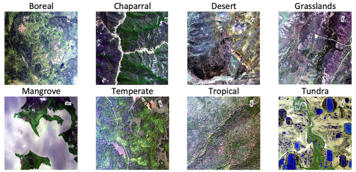
RGB composites of representative AVIRIS‐NG images.
Figure 2.

RGB composites of representative Portable Remote Imaging Spectrometer coastal ocean images.
We use actual spectra from three airborne hyperspectral instruments to represent realistic spatial, spectral, and noise characteristics. The Airborne Visible InfraRed Imaging Spectrometer ‐ Next Generation (AVIRIS‐NG) is an airborne spectrometer that acquires data in the spectral range 380–2,510 nm; the orthorectified and atmospherically corrected reflectance product was obtained from https://avirisng.jpl.nasa.gov/dataportal/. The National Ecological Observatory Network (NEON) Airborne Observing Platforms acquire data in the spectral range 380–2,500 nm using spectrometers closely related to AVIRIS‐NG; the orthorectified and atmospherically corrected reflectance product was obtained from https://data.neonscience.org/data‐products/DP1.30006.001 (NEON, 2021). The Portable Remote Imaging Spectrometer (PRISM) is an airborne spectrometer that acquires data in the spectral range 350–1,050 nm; the orthorectified and atmospherically corrected reflectance product was obtained from https://prism.jpl.nasa.gov/dataportal/. PRISM has a spectral resolution of 2.83 nm, and the AVIRIS‐NG and NEON spectrometers have a spectral resolution of 5 nm. These spectrometers, along with the upcoming Earth Mineral dust source InvesTigation (EMIT) and the notional SBG spectrometer are described in Table 1.
Table 1.
AVIRIS‐NG, NEON, PRISM, EMIT, and SBG Instrument Performance Parameters
| Instrument | Spectral range | Spectral resolution | Spectral FWHM | Number of bands |
|---|---|---|---|---|
| AVIRIS‐NG | 380–2,510 nm | 5 nm | 5 nm | 425 |
| NEON | 380–2,500 nm | 5 nm | 7.5 nm | 426 |
| PRISM | 350–1,050 nm | 2.8 nm | 3.5 nm | 92 |
| EMIT | 380–2,500 nm | 7.4 nm | 8.5 nm | 288 |
| SBG‐VSWIR (notional) | 400–2,500 nm | 5–10 nm | TBD | TBD |
A wide range of scenes was considered over different landcover types, spatial regions, and seasons to encapsulate a wide range of conditions. Each scene is described in Table 2, and further detail is provided in Appendix B. As a default, each image is resampled to 30 m GSD using bilinear interpolation, and the spectral bands are resampled to 10 nm spectral channels unless specified otherwise. Bands that may be impacted by water vapor or other artifacts (<400, 1,260–1,560, 1,760–1,960, and >2,450 nm) were excluded before computing the ID.
Table 2.
A List of the AVIRIS‐NG, NEON, and PRISM Images Used to Evaluate Intrinsic Dimensionality
| Biome | Location | #Bands | GSD | Sensor | Date of acquisition |
|---|---|---|---|---|---|
| Chaparral | California | 432 | 3.7 m | AVIRIS‐NG | 2014‐06‐03 |
| Desert a | Nevada | 432 | 3.7 m | AVIRIS‐NG | 2014‐06‐25 |
| Mangrove | Louisiana | 432 | 3.8 m | AVIRIS‐NG | 2015‐05‐09 |
| Temperate Forest | Wisconsin | 432 | 4.4 m | AVIRIS‐NG | 2015‐09‐04 |
| Dry Tropical Forest a | India | 425 | 3.6 m | AVIRIS‐NG | 2016‐01‐07 |
| Grasslands | Oklahoma | 425 | 3.1 m | AVIRIS‐NG | 2017‐06‐14 |
| Tundra | Alaska | 425 | 5.3 m | AVIRIS‐NG | 2018‐07‐29 |
| Boreal Forest | Canada | 425 | 5.1 m | AVIRIS‐NG | 2018‐08‐11 |
| Wetlands | Florida (OSBS) | 426 | 1 m | NEON | 2019‐04‐16 |
| Mixed Forest | Michigan (UNDE) | 426 | 1 m | NEON | 2019‐06‐06 |
| Grasslands | Kansas (KONZ) | 426 | 1 m | NEON | 2019‐07‐12 |
| Evergreen Forest | Alabama (DELA) | 426 | 1 m | NEON | 2019‐04‐29 |
| Mixed Forest | California (SOAP) | 426 | 1 m | NEON | 2019‐06‐14 |
| Mixed Forest | California (TEAK) | 426 | 1 m | NEON | 2019‐06‐14 |
| Coral Reef | Australia | 92 | 7.9 m | PRISM | 2016‐09‐17 |
| Coral Reef | Hawaii | 92 | 7.8 m | PRISM | 2017‐03‐06 |
| Coral Reef | Palau | 92 | 8 m | PRISM | 2017‐05‐16 |
Note. The difference in the number of available bands for AVIRIS‐NG between 2015 and 2016 reflects changes made to the internal processing pipeline. The total number of bands reflects the original image size, before masking of bands that may be influenced by atmospheric effects.
These two scenes were processed to reflectance separately using the optimal estimation algorithm in ISOFIT (Thompson et al., 2018) and evaluated manually to ensure the best atmospheric correction.
While most scenes were downloaded in their publicly available form, two scenes were specially processed: the desert scene in Nevada and the dry tropical forest in India. In certain images, slight artifacts remain after standard atmospheric correction. Ordinarily, this is not of great concern, and the ID computation was not significantly impacted by these features. However, for the SNR experiments, the noise needed to be added at the sensor level. When a spectrum containing artifacts is propagated back through a modeled atmosphere, and noise is then added, these features are amplified in the final atmospheric correction, adding extraneous noise that is not defined by the SNR input. In order to minimize introduction of additional noise, the Nevada and India scenes were atmospherically corrected using the Imaging Spectrometer Optimal FITting (ISOFIT) tool (Thompson et al., 2018) and manually evaluated for the best correction. ISOFIT is an atmospheric correction tool which performs Maximum a Posteriori inversion of a forward radiative transfer model. In our configuration, the state vector contains atmospheric variables such as water vapor and aerosol optical depth in addition to surface reflectance. A nonlinear optimization finds the optimal state configuration to match the predicted radiance to the actual measurement, while accounting for the uncertainty due to instrument noise and systematic calibration errors. The forward model can accommodate any radiative transfer assumptions including variable viewing angles and elevations within a scene. The code has been validated across many airborne campaigns (Brodrick et al., 2022; Greenberg et al., 2022; Thompson et al., 2019) and is being used by the EMIT mission (Connelly et al., 2021). ISOFIT is publicly available via Zenodo.
The SBG mission architecture described in the 2017 Earth Science and Applications from Space Decadal Survey (National Academies of Sciences, Engineering, & Medicine, 2018) consists of high‐GSD visible‐to‐shortwave infrared hyperspectral and multi‐channel TIR imagers. The AVIRIS‐NG and NEON data sets are very good proxies for the VSWIR spectrometer and were used to evaluate GSD, spectral resolution, and SNR. Because the thermal imager will be a multiband (<10 channels) instrument, spectral dimensionality is not an appropriate metric. However, the thermal instrument was considered in the temporal resolution assessment in Section 4.
3.2. Simulation Environment
The Py‐Hypertrace environment enables users to simulate accurate spectral imagery given as input a reflectance (“truth”) image. The forward model uses sRTMnet (Brodrick et al., 2021) to simulate sensor noise, view and sun geometry, and atmospheric spectral signatures. The inverse model uses ISOFIT to retrieve the atmospheric parameters and surface reflectance simultaneously, and the difference between the true and estimated reflectance images provides an estimate of accuracy. Py‐Hypertrace is available through the ISOFIT Zenodo repository.
Preliminary testing showed that the spatial and spectral resolution experiments were unchanged when running through ISOFIT or on the original reflectance product, so Hypertrace was only used for the SNR experiment. In addition, some publicly available reflectance products had minor spectral artifacts from atmospheric correction. While these are often inconsequential, in this case, adding atmosphere and noise enhanced artifacts and often dominated the signal. Because of this, only the two scenes with negligible artifacts (Nevada and India) were used for the SNR experiment.
By default, our Hypertrace runs assumed a “mid‐latitude summer” atmospheric profile (a standard MODTRAN atmosphere defined in Anderson et al., 1986), an aerosol optical depth of 0.1, an atmospheric water vapor content of 1 cm, a nadir viewing angle, and a 10:00 local solar time acquisition (solar zenith angle of 37.21° and solar azimuthal angle of 53.82°, at the equator on the 200th day of the year). These atmospheric parameters are fixed in the forward model, and the inverse model independently solves for the aerosol optical depth and atmospheric water vapor content in addition to the surface reflectance profile.
Realistic SNR was simulated using an instrument model that considers detector design parameters to account for different noise sources, including dark current, electronic readout noise, etc. It also includes precise calculation of photon shot noise based on efficiencies of the instrument components, internal reflections off telescope surfaces, throughput loss due to grating, dark current, electronic readout, etc (described in detail in Thompson et al., 2020). The noise depends on signal and wavelength and is drawn from a multivariate Gaussian distribution defined by three parameters, such that the noise‐equivalent change in radiance , where is the observed radiance at the center wavelength of each spectral band (Thompson et al., 2020). The parameters we used were modeled for the EMIT instrument, a spectrometer that will launch in 2022 and will serve as a precursor instrument to SBG (Connelly et al., 2021). EMIT is also closely related to AVIRIS‐NG and the NEON instruments in terms of spectral resolution, range, number of channels, and SNR (see Table 1).
3.3. Temporal Resolution
While the GSD, spectral resolution, and SNR could be evaluated using existing airborne hyperspectral data sets, there are currently insufficient hyperspectral data that is sampled frequently enough (less than 5 days revisit over at least one annual cycle) for a sensitivity study of temporal resolution. Instead, we have used daily multispectral data as a proxy. In this case, the image matrix is of size , where is the number of temporal observations, and the image covariance matrix will be size . Spectral dimensionality has been well established as a metric in other applications, but to our knowledge, this is the first use of temporal dimensionality. Instead of determining unique classes by their spectral features, we are now defining classes by phenological patterns. For example, while the normalized difference vegetation index (NDVI) over deserts might remain essentially unchanged, the NDVI of forests will fluctuate according to seasonal change, and different crops will be separable by their planting and harvest times. With fewer observations, all crops planted within a single season might be grouped, but frequent observations would result in higher information content. The temporal patterns seen in multispectral data have already been incorporated into the classification of agricultural and unmanaged landscapes (e.g., J. Chang et al., 2007; Foerster et al., 2012; Lobell & Asner, 2004; Sakamoto et al., 2005; Zhang et al., 2003).
The Visible Infrared Imaging Radiometer Suite (VIIRS) acquires daily optical data globally in 22 spectral channels at two GSDs: 375 and 750 m. These were resampled to 1 km for consistency with MODIS heritage, and five bands (bands I1‐5) were resampled to 500 m GSD. This daily global data set forms a valuable basis for studying the impact of revisit time on information content. We used two VIIRS standard products in this analysis: the VNP43IA4.001 nadir BRDF‐adjusted daily reflectance product at 500 m (Schaaf et al., 2018); and the VNP21A1D.001 land surface temperature (LST) and emissivity daytime product at 1 km (Hulley & Hook, 2018). The red high‐resolution reflectance band I1 was used to evaluate temporal dimensionality in the visible part of the spectrum. The daily LST product was used to evaluate temporal dimensionality in the TIR.
We evaluated 11 sites in highly biodiverse regions (Myers et al., 2000), as well as two agricultural regions, described in Table 3 and shown in Figure 3. All products were cropped to the area of interest and downloaded using AppEEARs (AppEEARS, 2021). The site extents are provided in Appendix B.
Table 3.
VIIRS Sites Used to Evaluate Temporal Dimensionality
| Biome | Location | Site size (km2) | a Date of acquisition |
|---|---|---|---|
| Southwest Australia | Australia | 48,000 | Jan–Dec 2020 |
| Amazon Forest | Brazil | 34,000 | Jan–Dec 2020 |
| Caucasus | Bulgaria | 20,000 | Jan–Dec 2020 |
| Boreal Forest | Canada | 28,000 | Jan–Dec 2020 |
| Tropical Forest | Democratic Republic of Congo | 51,000 | Jan–Dec 2020 |
| Eastern Afromontane | Ethiopia | 41,000 | Jan–Dec 2020 |
| Mediterranean Basin | Portugal | 42,000 | Jan–Dec 2020 |
| Boreal Forest | Russia | 27,000 | Jan–Dec 2020 |
| Cape Floristic Region | South Africa | 5,000 | Jan–Dec 2020 |
| Indo‐Burma Biodiversity Hotspot | Thailand | 112,000 | Jan–Dec 2020 |
| Sierra Nevada | USA (California) | 14,000 | Jan–Dec 2020 |
| Agriculture | USA (California) | 12,000 | Jan– Dec 2020 |
| Agriculture | USA (Iowa) | 32,000 | Jan–Dec 2020 |
Daily reflectance and LST were retrieved for each site.
Figure 3.
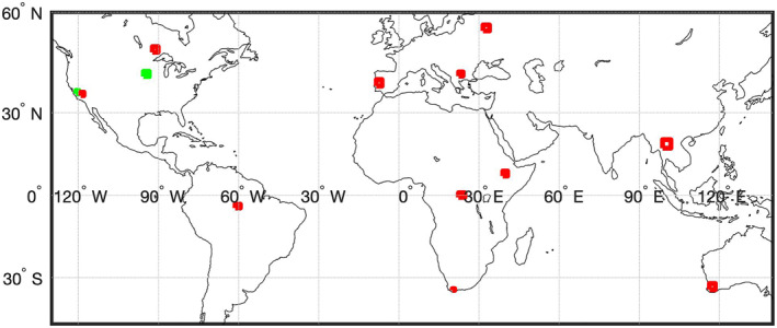
The biodiversity hotspots (red) and agricultural regions (green) selected for temporal dimensionality evaluation. See Table 3.
The VIIRS nadir BRDF‐adjusted daily reflectance product is accompanied by quality flags that indicate the complete inversion's success and quantify the impact of clouds. The daytime LST product is also accompanied by quality flags that indicate clouds, calibration quality, and algorithm convergence speed. Only the best quality pixels were used. For both products, pixels containing fill values were also discarded.
Each image contained between 20,000 and 500,000 pixels (each manually selected to capture landcover heterogeneity). For each pixel, a time series was constructed for reflectance band I1 and LST, building up three‐dimensional image stacks that are similar in format to a hyperspectral image. Images at a particular timestamp were removed from analysis where more than 20% of the image was masked due to cloud or other flags indicated lower quality data. The resulting image and noise estimates were used as inputs in the RMT method to determine the temporal dimensionality. This method was repeated for different temporal sampling strategies. The image stack was sampled at regular intervals to simulate different revisit frequencies (i.e., to simulate a 16‐day revisit cycle, only every 16th observation was used to compute the temporal dimensionality. If that 16th observation was cloudy in the VIIRS data, then it would not be used as input into the ID computation). The increasing temporal gap between observations necessitated Meer's method to estimate the noise since the statistical methods rely on a high correlation between neighboring observations to compute the noise contribution.
To demonstrate that temporal dimensionality translates to real quantities, we compared it to estimates of peak greenness over the California agricultural site. To derive peak greenness, we compiled a temporal stack of NDVI, as described for I1 and LST above. We define NDVI = (I2 – I1)/(I2 + I1), where I2 is the VIIRS high‐resolution near‐infrared band. Five hundred pixels were randomly selected for analysis, and each pixel was processed to better represent the seasonal growing cycle. This was repeated for five different start times to reduce the effect of revisit periodicity linking up with a seasonal peak, yielding 2,500‐time series vectors. First, the pixel was subsampled to the revisit period under consideration; any gaps were filled using forward and reverse autoregressive fits from the remaining time series; outliers were removed, where outliers were defined as points more than three standard deviations from the mean of a 5‐point moving window; and a squared exponential curve approximation was used to represent the time series while removing unexpected drops in NDVI due to undetected cloud. Finally, the maximum value of the squared exponential curve is set as the peak greenness.
4. Experiments and Results
4.1. Ground Sampling Distance
To quantify the impact of GSD on ID, we evaluated the ID for all scenes listed in Table 2, resampled to GSDs of 5, 10, 20, 30, 40, 50, and 60 m. In each case, the original image was spatially resampled using bilinear interpolation, and all images were resampled to a fixed spectral resolution of 10 nm. No additional noise was added to the original reflectance images, which means that the coarser resolution images have a higher SNR due to the averaging effect. This is in line with the assumption that a real instrument with larger GSD will have longer integration time per pixel and therefore a higher SNR. This is discussed further in Raiho et al. (2022), and explored in more detail in further experiments described below. Since the atmospheric correction is run pixel‐by‐pixel, there was no need to include additional instrument or atmospheric parameters beyond the original reflectance product.
We calculated the ID for each scene from Table 2 at every GSD using RMT and the multiple regression noise estimation described in Section 2. For each scene, the ID was normalized to the ID calculated for the GSD = 5 m case. The normalized ID value was used since there was a large amount of variation in the information content of each scene (ranging from ID = 3 in the Great Barrier Reef to ID = 34 in the boreal forest at 10 nm spectral resolution and 30 m GSD). Figure 4 shows that the normalized IDs (NID) decrease as GSD increases, but there is a significant variation at coarser GSD since heterogeneous scenes are more sensitive to GSD than homogeneous scenes. On average, images from an instrument with a 60 m GSD will have roughly 30% lower information content than images from an instrument with a 30 m GSD.
Figure 4.
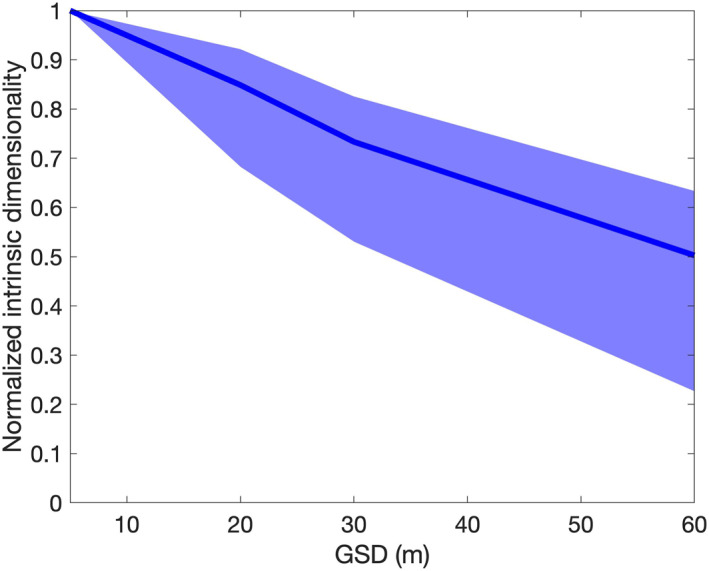
Intrinsic dimensionality (ID) decreases with larger pixel sizes. The thick line shows the median ID across all 17 scenes, and the shaded area encompasses the 25th–75th percentile of normalized IDs across all scenes. The ID values are normalized to a reference ID at 5 m GSD.
We recognize that the bilinear interpolation we used to resample our images spatially might average out some of the noise, thereby conflating two variables. To account for this, we estimated the noise present in the image (already done as part of the ID computation). We added Gaussian noise so that the overall standard deviation of noise in each band remained similar for each image. One image, in particular, was an outlier to Figure 4. The NEON evergreen forest site DELA had ID values of 8, 7, 8, 11 for GSDs of 30, 40, 50, 60 m. We hypothesized that a higher ID at 60 m (contrary to Figure 4) was due to the noise suppression of the image resampling. When we included additional noise, the ID values became 8, 7, 7, 7 for GSDs of 30, 40, 50, 60 m. This progression is more in line with the other data sets. More telling is that the other data sets captured in the 25th–75th percentile shading shown in Figure 4 did not change ID values when noise consistency was ensured. We conclude that images that are especially sensitive to noise may behave differently, but overall the ID analysis of resampled reflectance imagery was robust.
Another area worth considering is the impact of the number of pixels on the overall analysis. The ID method, particularly when using a statistically derived noise estimate, does not utilize the spatially contiguous nature of a scene (i.e., the pixels could be randomly reordered without changing the ID). However, a certain number of pixels are required in order to meaningfully represent a scene. To illustrate this, we chose a diverse site (in this case the boreal forest AVIRIS‐NG image) and randomly subsampled the scene, computing ID on the subset. Figure 5 shows that a subsample of fewer than 500 pixels failed to accurately detect all the unique components within the scene. The other scenes performed similarly, with less complex scenes having a lower limit for the required number of pixels.
Figure 5.
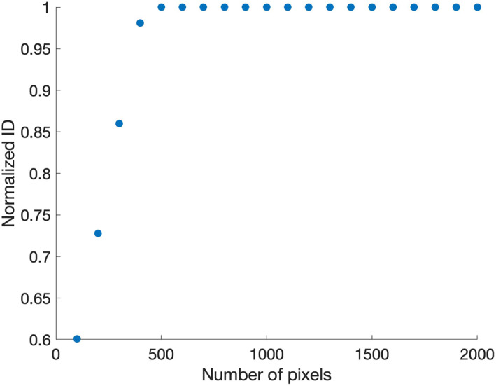
When evaluating diverse sites, such as the boreal forest scene shown here, the intrinsic dimensionality (ID) is not accurately determined once fewer than 500 pixels are sampled.
4.2. Spectral Resolution
To quantify the impact of spectral resolution on ID, we evaluated the ID for all scenes listed in Table 2 spectrally resampled to 5, 15, 20, 25, and 30 nm. In each case, the original image was spectrally resampled using linear interpolation, and all images were resampled to a fixed GSD of 30 m. No additional noise was added to the original reflectance images.
Using RMT and the multiple regression noise estimation described in Section 2, we calculated the ID for each scene at each spectral resolution. For each scene, the ID was normalized to the ID calculated for the spectral resolution = 5 nm case. Figure 6 shows that the scaled ID decreases as spectral resolution varies from 5 to 30 nm, with a relatively steep drop‐off from 5 nm and less variation than seen in Figure 4. In this case, changing the spectral resolution could also impact the atmospheric correction by affecting the ability to measure spectrally sharp water vapor absorption features. We tested this by running Hypertrace simulations on two scenes (Nevada and India) and comparing the results to the spectral resampling performed on the original reflectance data. Figure 6 shows that coarser spectral resolution does impact the atmospheric correction, resulting in slightly lower ID values, but the overall shape remains comparable. There is an information loss of ∼40% moving from 10 to 20 nm spectral resolution.
Figure 6.
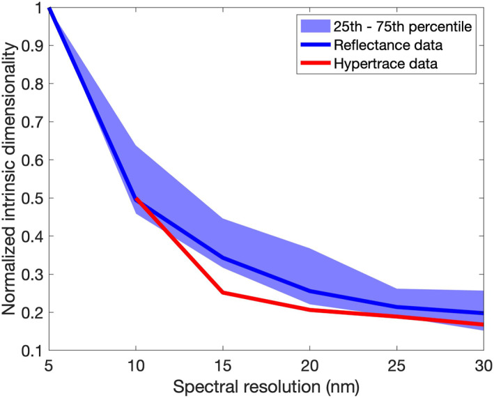
Normalized intrinsic dimensionality (ID) decreases with coarser spectral resolution. The thick blue line shows the median ID across all scenes, and the shaded area encompasses the 25th–75th percentile of scaled ID across all scenes. The red curve (the average from the Nevada and India scenes) shows that coarser spectral resolution negatively impacts ID when considering atmospheric correction, but this effect is negligible (generally <10% of the maximum ID).
4.3. Signal‐To‐Noise Ratio
Unlike the GSD and spectral resolution experiments, realistic SNR could not be easily simulated at the reflectance level. Therefore, we used Hypertrace to simulate realistic radiance data using the atmospheric, instrument, and noise models and computed ID on the reflectance output using ISOFIT. SNR, in this case, was set by adjusting the integration time within the noise model—higher integration times meant increased signal and therefore a higher SNR, and vice versa.
As discussed in Section 3.1, only the Nevada and India scenes were used for the Hypertrace experiment to minimize the propagation of spectral artifacts. These images were resampled to 30 m GSD and 10 nm spectral resolution. We varied SNR by varying integration times in the simulation. We used integration times of 0.0015, 0.003, 0.0045, 0.006, 0.0075, 0.009 s which corresponded to average SNR values of approximately 170, 250, 300, 350, 390, and 430, respectively. Figure 7 shows that lower ID values are detected in noisier scenes since distinguishing spectral features may be obscured by high noise variance. Figure 8 shows the SNR values for all wavelengths for each choice of integration time.
Figure 7.
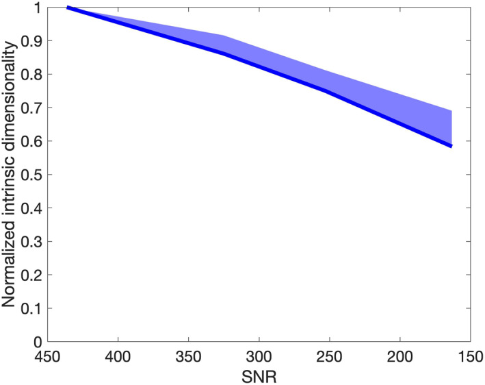
Intrinsic dimensionality (ID) decreases as the signal‐to‐noise ratio (SNR) decreases. Since only two scenes were considered here, the shading encapsulates the range of scaled ID between the Nevada and India scenes. Note that the x‐axis has been reversed, to reflect the decrease in ID from low noise (high SNR) to high noise (low SNR).
Figure 8.
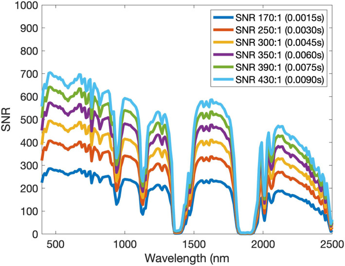
Signal‐to‐noise ratio (SNR) varies by channel, decreasing at longer wavelengths due to both lower radiance levels and higher noise. Here, the modeled SNR curve at each wavelength is shown for each choice of average SNR (with associated integration time). Note that the intense atmospheric water absorptions (SNR = 0) near 1,400 and 1,900 nm effectively remove all light from the spectrum, and these bands have been removed from the ID analysis.
4.4. Temporal Resolution
The tropical forest sites in South America (Brazil) and Central Africa (DRC) and the Boreal Forest in Northern Russia were cloud contaminated to the point of algorithm failure. This will be a problem to consider for SBG and other missions that hope to acquire data in these regions. We anticipate that SBG will have better sampling statistics due to its 30 m GSD; however, cloud shadows and other interferences may still make these challenging regions. These sites were removed from further analysis, leaving 11 remaining sites. Other sites such as Canada, Ethiopia, and Thailand had ID values that dropped to zero with revisits exceeding 4–8 days (in other words, with weekly sampling there were insufficient pixels to track over time for the ID computation). Figure 9 shows the decrease in NDVI temporal dimensionality with increased revisit time by combining the temporal ID estimates for all sites with ID > 0. There is rapid information loss in the 1–5 days revisit range, which would capture weather‐related phenological perturbations on synoptic time scales and separate classes with similar growth patterns. SBG anticipates a 16‐day revisit for the VSWIR instrument, but there is potential for harmonization with temporally intersecting missions, such as the ESA's Copernicus Hyperspectral Imaging Mission for the Environment (CHIME). We have shown the ID curve normalized (NID) by an 8‐day baseline to illustrate the benefits to harmonization (Figure 9). Moving from a 16‐day (NID ∼ 0.60) to a 30‐day revisit (NID ∼ 0.36) would result in the loss of about 40% of the dimensionality, which means that fewer classes would be seasonally separable. In contrast, a harmonized SBG‐CHIME data set that reduced the revisit time from 16 days (NID ∼ 0.60) to 8 days (NID ∼ 1.0) would increase the ID by 67%. This analysis is significantly impacted by clouds, which is a realistic problem that will be faced by all optical systems including SBG.
Figure 9.
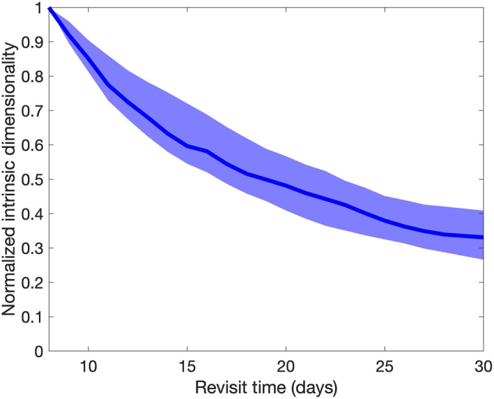
Temporal dimensionality of Visible Infrared Imaging Radiometer Suite band I1 normalized by the intrinsic dimensionality at 8‐day revisit is shown as a function of revisit time. Going from a 16‐day (proposed by SBG) to a 30‐day revisit results in approximately 40% of the information content being lost. The solid line represents the 50th percentile of all sites, and the shading represents the 25th and 75th percentiles.
Figure 10 shows the results of a similar experiment for LST, except here the dimensionality normalization was performed against a 1‐day revisit due to the intrinsic timescale of LST variability. This is reflected in the rapid decay of temporal dimensionality for the thermal regime compared to the VSWIR. As seen in the plot, the normalized ID decreases to ∼0.65 going from 1‐day to 2‐day revisit, drops to ∼0.40 for a 3‐day revisit, and is less than 0.20 for a 6‐day revisit. This is reasonable since evapotranspiration and LST change far more rapidly than vegetation greenness. There is potential for harmonization with the Indian Space Agency/French National Center for Space Studies TIR Imaging Satellite for High‐resolution Natural resource Assessment (TRISHNA) and the ESA's Copernicus Land Surface Temperature Monitoring missions. Harmonization between the three TIR missions could deliver an effective 1‐day global revisit, significantly enhancing the science return over what any of the three missions could achieve individually.
Figure 10.
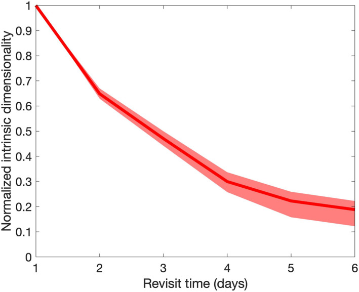
Temporal dimensionality of Visible Infrared Imaging Radiometer Suite daytime LST normalized by the intrinsic dimensionality at daily revisit is shown as a function of revisit time. There is a decrease in information content with increasing revisit time, with a faster decay than the visible. In going from a 3‐day to 6‐day revisit, approximately 60% of the information content is lost. The solid line represents the 50th percentile of all sites, and the shading represents the 25th and 75th percentiles.
Figure 11 shows that temporal dimensionality is a good proxy for ecosystem variables such as the NDVI value at peak greenness in their dependence on revisit. Estimates of maximum NDVI values can be biased by up to 5% with an increased revisit time. This suggests that peak NDVI is relatively slowly varying and is consistent with the ∼1 week time scale on which NDVI varies significantly. The dimensionality shows a much larger decrease (85%) in information content because it represents more than the simple metric of peak greenness and is analogous to the sum of the impact faced by a wide array of more complex algorithms.
Figure 11.
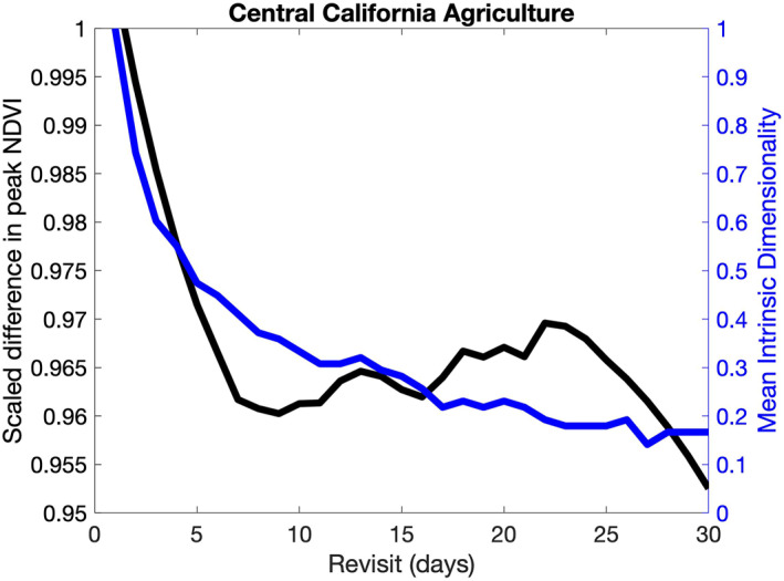
The difference in peak normalized difference vegetation index (NDVI), scaled by peak NDVI at a daily revisit (left), tracks well with dimensionality for different revisit times (left).
5. Discussion
We illustrate ID as a metric for mission design, and we have shown how ID is sensitive to changes in GSD, spectral resolution, SNR, and temporal resolution. Our experiments show that ID consistently decreased for larger pixels, wider spectral channels, lower SNR, and less frequent observations even over multiple different biomes. All of these results are as expected since we intuitively understand that large pixels will contain mixtures of many—sometimes small—objects, and their individual contribution to the overall pixel spectrum will be small; wider spectral channels will mean that spectrally narrow diagnostic spectral features will be undetectable; noise will overpower small‐amplitude spectral characteristics, and important events may not be adequately captured with infrequent acquisitions. While it might seem best to simply design a mission with the highest possible resolutions in all variables, realistically there are relationships and trade‐offs between these variables. For instance, the same detector could be used in a design to improve SNR by increasing GSD (due to increased integration time), but both parameters cannot be optimized at the same time. Similarly, the same detector with a different telescope could acquire small GSD (and consequently smaller swath) with infrequent acquisitions, or a wider swath (and consequently larger GSD) more frequently. In order to balance these trade‐offs, a consistent metric is needed. The importance of our investigation has been to demonstrate that ID is a consistent, objective, quantitative metric that can be used to measure expected performance over many mission design parameters and different landcover types.
In a traditional sensitivity analysis for remotely sensed products, the sensitivity will be dependent on the algorithm used to derive the product and will be in the associated product units. In a multi‐faceted mission such as SBG, how would one weigh the importance of for example, Kaolinite fractional abundance (%) relative to that of leaf mass per unit area (g/m2), or compare the accuracy of snow grain size ( m) to sulfur dioxide emissions from volcanoes (kt)? There is a critical need for an applications‐agnostic, data‐driven metric to enable a fair comparison. We propose that ID is such a metric.
We used airborne hyperspectral imagery over multiple biomes, including Chaparral, Desert, Mangrove, Temperate Forest, Dry Tropical Forest, Grasslands, Tundra, Boreal Forest, Coral Reefs, Agriculture, and Urban environments. There was some variability in response to GSD—some heterogeneous scenes experienced a significant drop in ID for coarser pixels, whereas homogeneous scenes were less sensitive. However, the response to spectral resolution was fairly consistent across all scenes, highlighting the importance of hyperspectral over multispectral data.
We also introduced the concept of temporal dimensionality, using phenological patterns to define information content over time, and using this to demonstrate the impact of revisit over both the VSWIR and TIR. This metric could also be used to evaluate optimal overpasses for complementary missions to maximize science value.
In future work, real instrument configurations can be compared to optimize data rates, determine the optimal configuration within a design space, cost savings can be paired with measurable science consequences, and data harmonization can be explored.
6. Conclusion
The SBG mission will be an essential part of the NASA Earth System Observatory, and optimal mission design is vital for answering science questions and meeting applications needs across diverse fields. Individual geophysical products relating to terrestrial and aquatic ecosystems, natural disasters, and the cryosphere might benefit from different mission design parameters according to each algorithm's unique sensitivities, and so overall mission optimization is difficult. Here we have introduced the concept of ID as a metric to be considered in future mission design since it provides a single quantitative evaluation for a combination of design parameters, irrespective of higher‐level algorithms, products, applications, or disciplines. ID is simple to compute, yet it captures the maximum data content achievable for a combination of parameters and indicates the potential of optimal algorithmic performance. We found that the ID decreases for coarser GSD, decreased spectral resolution, less frequent acquisitions, and lower signal‐to‐noise levels. This behavior impacts the quality and accuracy of all derived products. Furthermore, because ID is application‐agnostic, it can be applied to other hyperspectral missions in Earth and planetary sciences.
Acknowledgments
Support to all authors was provided by NASA and the Jet Propulsion Laboratory, California Institute of Technology and to PAT by NSF Macrosystems Biology and NEON Early Science award 1638720. This study was also supported by the Space‐based Imaging Spectroscopy and Thermal (SISTER) pathfinder, and the Surface Biology and Geology (SBG) project, a NASA Earth Science Designated Observable. The research described in this paper was carried out at the Jet Propulsion Laboratory, California Institute of Technology, under contract with the National Aeronautics and Space Administration. © 2022. All rights reserved. Government sponsorship is acknowledged. We thank reviewers Prof. Jeff Dozier and Prof. Charles M. Bachmann for their suggestions, which significantly improved the manuscript.
Appendix A.
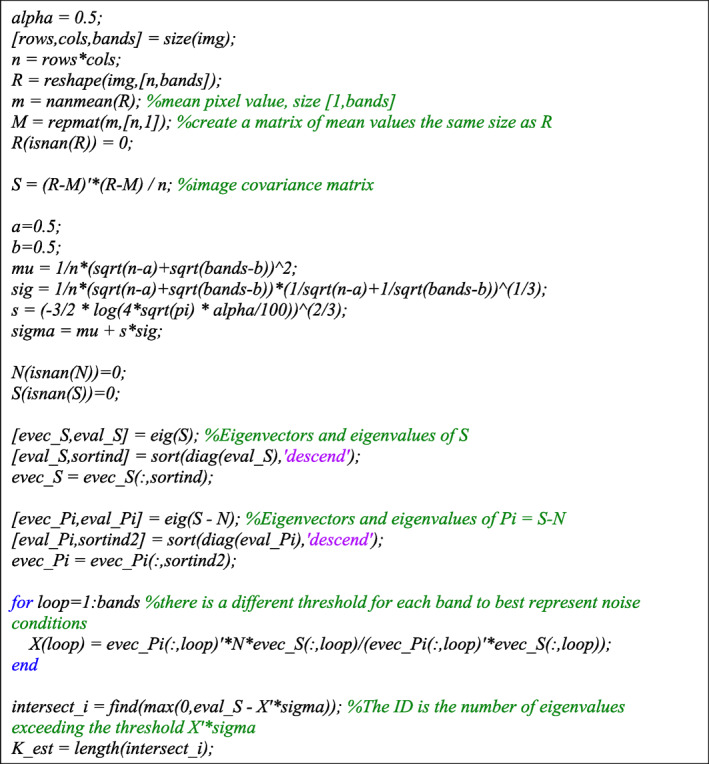
This appendix provides pseudocode for the ID calculation, as described in Cawse‐Nicholson et al. (2013). It assumes inputs of a 3‐dimensional hyperspectral image (“img”) of size rows x columns x bands, and a noise covariance matrix (“N”) of size bands x bands. One method for estimating the matrix “N” can be implemented in MATLAB using the publicly available code “estNoise.m” posted by Bioucas‐Dias and Nascimento (2008a, 2008b).
Appendix B.
Table B1 lists the filenames of the hyperspectral data sets used in this analysis. AVIRIS‐NG data can be downloaded from https://avirisng.jpl.nasa.gov/dataportal/; PRISM data can be downloaded from https://prism.jpl.nasa.gov/dataportal/; and the NEON data can be downloaded from https://data.neonscience.org/data‐products/DP1.30006.001.
Table B1.
The Filenames of the Hyperspectral Data Sets Used in This Analysis
| Biome | Location | Filename |
|---|---|---|
| Chaparral | California | ang20140603t185211_corr_v1e_img |
| Desert | Nevada | ang20140625_corr_v2gx_mosaic (*enhanced atmospheric correction) |
| Mangrove | Louisiana | ang20150509t213032_corr_v1e_img |
| Temperate Forest | Wisconsin | ang20150904t163629_corr_v1e.img |
| Dry Tropical Forest | India | ang20160107t062934_rfl (*enhanced atmospheric correction) |
| Grasslands | Oklahoma | ang20170614t171958_corr_v2p6_img |
| Tundra | Alaska | ang20180729t211026_corr_v2r2_img |
| Boreal Forest | Canada | ang20180811t212826_corr_v2r2_img |
| Wetlands | Florida (OSBS) | NEON_D03_OSBS_180.tif |
| NEON_D03_OSBS_181.tif | ||
| NEON_D03_OSBS_182.tif | ||
| Mixed Forest | Michigan (UNDE) | NEON_D05_UNDE_182.tif |
| NEON_D05_UNDE_183.tif | ||
| NEON_D05_UNDE_184.tif | ||
| Grasslands | Kansas (KONZ) | NEON_D06_KONZ_153.tif |
| NEON_D06_KONZ_153b.tif | ||
| NEON_D06_KONZ_154.tif | ||
| Evergreen Forest | Alabama (DELA) | NEON_D08_DELA_145.tif |
| NEON_D08_DELA_145b.tif | ||
| NEON_D08_DELA_150 | ||
| Mixed Forest | California (SOAP) | NEON_D17_SOAP_185.tif |
| NEON_D17_SOAP_191.tif | ||
| NEON_D17_SOAP_191b.tif | ||
| Mixed Forest | California (TEAK) | NEON_D17_TEAK_173.tif |
| NEON_D17_TEAK_173b.tif | ||
| NEON_D17_TEAK_174.tif | ||
| Coral Reef | Australia | prm20160917t001910_rb_v1w2_img |
| Coral Reef | Hawaii | prm20170306t194614_rb_v1w3_img |
| Coral Reef | Palau | prm20170516t003534_rb_v1w4_img |
- VIIRS/NPP BRDF/Albedo Nadir BRDF‐Adjusted Ref Daily L3 Global 500m SIN Grid V001.
- VIIRS/NPP Land Surface Temperature and Emissivity Daily L3 Global 1 km SIN Grid Day V001.
Table B2.
The Bounding Boxes (in Decimal Degrees) of the Visible Infrared Imaging Radiometer Suite Sites Used in the Temporal Analysis
| Biome | Min lat (°) | Mat lat (°) | Min lon (°) | Max lon (°) |
|---|---|---|---|---|
| Southwest Australia | −34.10 | −31.99 | 116.30 | 118.48 |
| Amazon Forest | −4.82 | −3.41 | −61.31 | −59.34 |
| Caucasus | 42.01 | 43.31 | 22.36 | 24.01 |
| Boreal Forest (Canada) | 49.18 | 50.80 | −92.29 | −90.14 |
| Tropical Forest (DRC) | −0.84 | 0.88 | 22.29 | 24.68 |
| Eastern Afromontane | 7.17 | 9.00 | 38.88 | 40.71 |
| Mediterranean Basin | 38.81 | 40.92 | −8.44 | −6.33 |
| Boreal Forest (Russia) | 55.16 | 56.74 | 31.50 | 33.93 |
| Cape Floristic Region | −34.31 | −33.75 | 20.00 | 20.88 |
| Indo‐Burma Biodiversity Hotspot | 17.44 | 20.53 | 98.72 | 101.81 |
| Sierra Nevada | 35.73 | 36.86 | −119.13 | −117.41 |
| Agriculture (California) | 36.33 | 37.44 | −120.92 | −119.87 |
| Agriculture (Iowa) | 41.86 | 43.47 | −95.63 | −93.46 |
Cawse‐Nicholson, K. , Raiho, A. M. , Thompson, D. R. , Hulley, G. C. , Miller, C. E. , Miner, K. R. , et al. (2022). Intrinsic dimensionality as a metric for the impact of mission design parameters. Journal of Geophysical Research: Biogeosciences, 127, e2022JG006876. 10.1029/2022JG006876
Data Availability Statement
AVIRIS‐NG reflectance data are available from https://avirisng.jpl.nasa.gov/dataportal/. NEON reflectance data are available from https://data.neonscience.org/data‐products/DP1.30006.001. The code for both ISOFIT and Hypertrace is available via Zenodo: https://doi.org/10.5281/zenodo.4614337.
References
- Anderson, G. P. , Clough, S. A. , Kneizys, F. X. , Chetwynd, J. H. , & Shettle, E. P. (1986). AFGL atmospheric constituent profiles (0.120 km). Air Force Geophysics Lab HANSCOM AFB MA. Retrieved from https://apps.dtic.mil/sti/pdfs/ADA175173.pdf [Google Scholar]
- AppEEARS Team . (2021). Application for Extracting and Exploring Analysis Ready Samples (AppEEARS). Ver. 2.63. NASA EOSDIS Land Processes Distributed Active Archive Center (LP DAAC), USGS/Earth Resources Observation and Science (EROS) Center. Retrieved 31 August 2021 from https://lpdaacsvc.cr.usgs.gov/appeears [Google Scholar]
- Asner, G. P. , Knapp, D. E. , Boardman, J. , Green, R. O. , Kennedy‐Bowdoin, T. , Eastwood, M. , et al. (2012). Carnegie Airborne Observatory‐2: Increasing science data dimensionality via high‐fidelity multi‐sensor fusion. Remote Sensing of Environment, 124, 454–465. 10.1016/j.rse.2012.06.012 [DOI] [Google Scholar]
- Bachmann, C. M. , Ainsworth, T. L. , & Fusina, R. A. (2008). Automated Estimation of Spectral Neighborhood Size in Manifold Coordinate Representations of Hyperspectral Imagery: Implications for Anomaly Finding, Bathymetry Retrieval, and Land Applications. Proc. IGARSS’08, Boston, MA, July 2008. 10.1109/IGARSS.2008.4778791 [DOI]
- Baik, J. , & Silverstein, J. W. (2006). Eigenvalues of large sample covariance matrices of spiked population models. Journal of Multivariate Analysis, 97(6), 1382–1408. 10.1016/j.jmva.2005.08.003 [DOI] [Google Scholar]
- Berman, M. (2019). Improved estimation of the intrinsic dimension of a hyperspectral image using random matrix theory. Remote Sensing, 11(9), 1049. 10.3390/rs11091049 [DOI] [Google Scholar]
- Bioucas‐Dias, J. M. , & Nascimento, J. M. (2005). Estimation of signal subspace on hyperspectral data. In Image and signal processing for remote sensing XI (Vol. 5982, p. 59820L). International Society for Optics and Photonics. 10.1117/12.620061 [DOI] [Google Scholar]
- Bioucas‐Dias, J. M. , & Nascimento, J. M. P. (2008a). Hyperspectral subspace identification. IEEE Transactions on Geoscience and Remote Sensing, 46, 2435–2445. 10.1109/TGRS.2008.918089 [DOI] [Google Scholar]
- Bioucas‐Dias, J. M. , & Nascimento, J. M. (2008b). HySime (hyperspectral signal subspace identification by minimum error) MATLAB code. Retrieved 28 April 2022 from http://www.lx.it.pt/~bioucas/code.htm
- Boardman, J. W. , & Green, R. O. (2000). Exploring the spectral variability of the Earth as measured by AVIRIS in 1999. Proceedings of the Ninth JPL Airborne Earth Science Workshop (Vol. 2000, pp. 195–206). JPL. [Google Scholar]
- Brodrick, P. G. , Thompson, D. R. , Fahlen, J. E. , Eastwood, M. L. , Sarture, C. M. , Lundeen, S. R. , et al. (2021). Generalized radiative transfer emulation for imaging spectroscopy reflectance retrievals. Remote Sensing of Environment, 261, 11247. 10.1016/j.rse.2021.112476 [DOI] [Google Scholar]
- Brodrick, P. G. , Thompson, D. R. , Garay, M. J. , Giles, D. M. , Holben, B. N. , & Kalashnikova, O. V. (2022). Simultaneous characterization of wildfire smoke and surface properties with imaging spectroscopy during the FIREX‐AQ field campaign. Journal of Geophysical Research: Atmospheres, 127, e2021JD034905. 10.1029/2021JD034905 [DOI] [PMC free article] [PubMed] [Google Scholar]
- Cawse‐Nicholson, K. , Damelin, S. B. , Robin, A. , & Sears, M. (2012). Determining the intrinsic dimension of a hyperspectral image using random matrix theory. IEEE Transactions on Image Processing, 22(4), 1301–1310. 10.1109/TIP.2012.2227765 [DOI] [PubMed] [Google Scholar]
- Cawse‐Nicholson, K. , Damelin, S. B. , Robin, A. , & Sears, M. (2013). Determining the intrinsic dimension of a hyperspectral image using random matrix theory. IEEE Transactions on Image Processing, 22(4), 1301–1310. 10.1109/TIP.2012.2227765 [DOI] [PubMed] [Google Scholar]
- Cawse‐Nicholson, K. , Hook, S. J. , Miller, C. E. , & Thompson, D. R. (2019). Intrinsic dimensionality in combined visible to thermal infrared imagery. IEEE Journal of Selected Topics in Applied Earth Observations and Remote Sensing, 12(12), 4977–4984. 10.1109/JSTARS.2019.2938883 [DOI] [Google Scholar]
- Cawse‐Nicholson, K. , Townsend, P. A. , Schimel, D. , Assiri, A. M. , & Blake, P. L. , et al. (2021). NASA's Surface Biology and Geology designated observable: A perspective on surface imaging algorithms. Remote Sensing of Environment, 257, 112349. 10.1016/j.rse.2021.112349 [DOI] [Google Scholar]
- Chang, C. I. , & Du, Q. (2004). Estimation of number of spectrally distinct signal sources in hyperspectral imagery. IEEE Transactions on Geoscience and Remote Sensing, 42(3), 608–619. 10.1109/TGRS.2003.819189 [DOI] [Google Scholar]
- Chang, C.‐I. , & Heinz, D. C. (2000). Constrained subpixel target detection for remotely sensed imagery. IEEE Transactions on Geoscience and Remote Sensing, 38(3), 1144–1159. 10.1109/36.843007 [DOI] [Google Scholar]
- Chang, C. I. , Wu, C. C. , Liu, W. , & Ouyang, Y. C. (2006). A new growing method for simplex‐based endmember extraction algorithm. IEEE Transactions on Geoscience and Remote Sensing, 44(10), 2804–2819. 10.1109/TGRS.2006.881803 [DOI] [Google Scholar]
- Chang, J. , Hansen, M. C. , Pittman, K. , Carroll, M. , & DiMiceli, C. (2007). Corn and soybean mapping in the United States using MODIS time‐series data sets. Agronomy Journal, 99(6), 1654–1664. 10.2134/agronj2007.0170 [DOI] [Google Scholar]
- Connelly, D. S. , Thompson, D. R. , Mahowald, N. M. , Li, L. , Carmon, N. , Okin, G. S. , & Green, R. O. (2021). The EMIT mission information yield for mineral dust radiative forcing. Remote Sensing of Environment, 258, 112380. 10.1016/j.rse.2021.112380 [DOI] [Google Scholar]
- Crisp, D. , Atlas, R. M. , Breon, F. M. , Brown, L. R. , Burrows, J. P. , Ciais, P. , & Schroll, S. (2004). The Orbiting Carbon Observatory (OCO) mission. Advances in Space Research, 34(4), 700–709. 10.1016/j.asr.2003.08.062 [DOI] [Google Scholar]
- Dierssen, H. M. , Ackleson, S. G. , Joyce, K. E. , Hestir, E. L. , Castagna, A. , Lavender, S. , & McManus, M. A. (2021). Living up to the hype of hyperspectral aquatic remote sensing: Science, resources, and outlook. Frontiers in Environmental Science, 9, 649528. 10.3389/fenvs.2021.649528 [DOI] [Google Scholar]
- Duren, R. M. , Thorpe, A. K. , Foster, K. T. , Rafiq, T. , Hopkins, F. M. , Yadav, V. , et al. (2019). California’s methane super‐emitters. Nature, 575, 180–184. 10.1038/s41586-019-1720-3 [DOI] [PubMed] [Google Scholar]
- Eldering, A. , Wennberg, P. O. , Crisp, D. , Schimel, D. S. , Gunson, M. R. , Chatterjee, A. , et al. (2017). The Orbiting Carbon Observatory‐2 early science investigations of regional carbon dioxide fluxes. Science, 358(6360). 10.1126/science.aam5745 [DOI] [PMC free article] [PubMed] [Google Scholar]
- Fisher, J. B. , Lee, B. , Purdy, A. J. , Halverson, G. H. , Dohlen, M. B. , Cawse‐Nicholson, K. , et al. (2020). ECOSTRESS: NASA’s next generation mission to measure evapotranspiration from the International Space Station. Water Resources Research, 56(4), e2019WR026058. 10.1029/2019WR026058 [DOI] [Google Scholar]
- Foerster, S. , Kaden, K. , Foerster, M. , & Itzerott, S. (2012). Crop type mapping using spectral‐temporal profiles and phenological information. Computers and Electronics in Agriculture, 89, 30–40. 10.1016/j.compag.2012.07.015 [DOI] [Google Scholar]
- Francis, P. , & Rothery, D. (2000). Remote sensing of active volcanoes. Annual Review of Earth and Planetary Sciences, 28(1), 81–106. 10.1146/annurev.earth.28.1.81 [DOI] [Google Scholar]
- Greenberg, E. , Thompson, D. R. , Jensen, D. J. , Townsend, P. A. , Queally, N. , Chlus, A. , et al. (2022). An improved scheme for correcting remote spectral surface reflectance simultaneously for terrestrial BRDF and water‐surface sunglint in coastal environments. Journal of Geophysical Research: Biogeosciences, 127, e2021JG006712. 10.1029/2021JG006712 [DOI] [Google Scholar]
- Hulley, G. , & Hook, S. (2018). VIIRS/NPP Land Surface Temperature and Emissivity Daily L3 Global 1 km SIN Grid Day V001. NASA EOSDIS Land Processes DAAC. Retrieved 20 August 2021 from 10.5067/VIIRS/VNP21A1D.001 [DOI]
- IPCC . (2021). Climate change 2021: The physical science basis. Contribution of Working Group I to the Sixth Assessment Report of the Intergovernmental Panel on Climate Change. In Masson‐Delmotte V., Zhai P., Pirani A., Connors S. L., Péan C., Berger S., et al. (Eds.), Cambridge University Press. In Press. Retrieved from https://www.ipcc.ch/report/ar6/wg1/ [Google Scholar]
- Jackson, T. J. , Bindlish, R. , Cosh, M. H. , Zhao, T. , Starks, P. J. , Bosch, D. D. , et al. (2011). Validation of Soil Moisture and Ocean Salinity (SMOS) soil moisture over watershed networks in the U.S. IEEE Transactions on Geoscience and Remote Sensing, 50(5), 1530–1543. 10.1109/TGRS.2011.2168533 [DOI] [Google Scholar]
- Johnstone, I. M. (2001). On the distribution of the largest eigenvalue in principal components analysis. Annals of Statistics, 295–327. 10.1214/aos/1009210544 [DOI] [Google Scholar]
- Kerr, Y. H. , Waldteufel, P. , Wigneron, J. P. , Martinuzzi, J. A. M. J. , Font, J. , & Berger, M. (2001). Soil moisture retrieval from space: The Soil Moisture and Ocean Salinity (SMOS) mission. IEEE Transactions on Geoscience and Remote Sensing, 39(8), 1729–1735. 10.1109/36.942551 [DOI] [Google Scholar]
- Kritchman, S. , & Nadler, B. (2008). Determining the number of components in a factor model from limited noisy data. Chemometrics and Intelligent Laboratory Systems, 94(1), 19–32. 10.1016/j.chemolab.2008.06.002 [DOI] [Google Scholar]
- Landerer, F. W. , Flechtner, F. M. , Save, H. , Webb, F. H. , Bandikova, T. , Bertiger, W. I. , et al. (2020). Extending the global mass change data record: GRACE Follow‐On instrument and science data performance. Geophysical Research Letters, 47(12), e2020GL088306. 10.1029/2020GL088306 [DOI] [Google Scholar]
- Landerer, F. W. , & Swenson, S. C. (2012). Accuracy of scaled GRACE terrestrial water storage estimates. Water Resources Research, 48(4). 10.1029/2011WR011453 [DOI] [Google Scholar]
- Lobell, D. B. , & Asner, G. P. (2004). Cropland distributions from temporal unmixing of MODIS data. Remote Sensing of Environment, 93(3), 412–422. 10.1016/j.rse.2004.08.002 [DOI] [Google Scholar]
- Myers, N. , Mittermeier, R. A. , Mittermeier, C. G. , Da Fonseca, G. A. , & Kent, J. (2000). Biodiversity hotspots for conservation priorities. Nature, 403(6772), 853–858. 10.1038/35002501 [DOI] [PubMed] [Google Scholar]
- Nascimento, J. M. , & Bioucas Dias, J. M. (2005). Vertex component analysis: A fast algorithm to unmix hyperspectral data. IEEE Transactions on Geoscience and Remote Sensing, 43(4), 898–910. 10.1109/TGRS.2005.844293 [DOI] [Google Scholar]
- National Academies of Sciences, Engineering, & Medicine . (2018). Thriving on our changing planet: A decadal strategy for Earth observation from space. National Academies Press. 10.17226/24938 [DOI] [Google Scholar]
- NEON (National Ecological Observatory Network) . (2021). Spectrometer orthorectified surface directional reflectance ‐ flightline, RELEASE‐2021 (DP1.30006.001). [Data set]. NOAA. 10.48443/n3ys-2070. . Retrieved 5 September 2021 from https://data.neonscience.org [DOI]
- Park, H. M. , Jung, H. Y. , Lee, T. W. , & Lee, S. Y. (1999). Subband‐based blind signal separation for noisy speech recognition. Electronics Letters, 35(23), 2011–2012. 10.1049/el:19991358 [DOI] [Google Scholar]
- Pascolini‐Campbell, M. , Fisher, J. B. , & Reager, J. T. (2021). GRACE‐FO and ECOSTRESS synergies constrain fine‐scale impacts on the water balance. Geophysical Research Letters, 48, e2021GL093984. 10.1029/2021GL093984 [DOI] [Google Scholar]
- Raiho, A. M. , Cawse‐Nicholson, K. , Chlus, A. , Dozier, J. , Gierach, M. , Miner, K. , et al. (2022). Exploring mission design for imaging spectroscopy retrievals for land and aquatic ecosystems. Journal of Geophysical Research: Biogeosciences. 10.1002/essoar.10510949.1 [DOI] [Google Scholar]
- Sakamoto, T. , Yokozawa, M. , Toritani, H. , Shibayama, M. , Ishitsuka, N. , & Ohno, H. (2005). A crop phenology detection method using time‐series MODIS data. Remote Sensing of Environment, 96(3–4), 366–374. 10.1016/j.rse.2005.03.008 [DOI] [Google Scholar]
- Schaaf, C. , Wang, Z. , Zhang, X. , & Strahler, A. (2018). VIIRS/NPP BRDF/Albedo Nadir BRDF‐Adjusted Ref Daily L3 Global 500m SIN Grid V001. NASA EOSDIS Land Processes DAAC. 10.5067/VIIRS/VNP43IA4.001 [DOI]
- Schmidt, R. , Schwintzer, P. , Flechtner, F. , Reigber, C. , Güntner, A. , Döll, P. , et al. (2006). GRACE observations of changes in continental water storage. Global and Planetary Change, 50(1–2), 112–126. 10.1016/j.gloplacha.2004.11.018 [DOI] [Google Scholar]
- Small, C. (2001). Multiresolution analysis of urban reflectance. Proceedings of the IEEE/ISPRS Joint Workshop 2001: Remote sensing and data fusion over urban areas (Vol. 2001, pp. 15–19). IEEE. [Google Scholar]
- Stavros, E. N. , Chrone, J. , Cawse‐Nicholson, K. , Freeman, A. , Glenn, N. , Guild, L. , et al. (2022). Designing an observing system to study the Surface Biology and Geology (SBG) of the Earth in the 2020s. JGR Biogeosciences, 127, e2021JG006471. 10.1029/2021JG006471 [DOI] [PMC free article] [PubMed] [Google Scholar]
- Swayze, G. A. , Clark, R. N. , Goetz, A. F. , Chrien, T. G. , & Gorelick, N. S. (2003). Effects of spectrometer band pass, sampling, and signal‐to‐noise ratio on spectral identification using the Tetracorder algorithm. Journal of Geophysical Research: Planets, 108(E9). 10.1029/2002JE001975 [DOI] [Google Scholar]
- Thompson, D. R. , Babu, K. N. , Braverman, A. , Eastwood, M. , Green, R. O. , Hobbs, J. , et al. (2019). Optimal estimation of spectral surface reflectance in challenging atmospheres. Remote Sensing of Environment, 232, 111258. 10.1016/j.rse.2019.111258 [DOI] [Google Scholar]
- Thompson, D. R. , Boardman, J. W. , Eastwood, M. L. , & Green, R. O. (2017). A large airborne survey of Earth’s visible‐infrared spectral dimensionality. Optics Express, 25(8), 9186–9195. 10.1364/OE.25.009186 [DOI] [PubMed] [Google Scholar]
- Thompson, D. R. , Braverman, A. , Brodrick, P. G. , Candela, A. , Carmon, N. , Clark, R. N. , et al. (2020). Quantifying uncertainty for remote spectroscopy of surface composition. Remote Sensing of Environment, 247, 111898. 10.1016/j.rse.2020.111898 [DOI] [Google Scholar]
- Thompson, D. R. , Natraj, V. , Green, R. O. , Helmlinger, M. C. , Gao, B. C. , & Eastwood, M. L. (2018). Optimal estimation for imaging spectrometer atmospheric correction. Remote Sensing of Environment, 216, 355–373. 10.1016/j.rse.2018.07.003 [DOI] [Google Scholar]
- Winter, M. E. (1999). An algorithm for fast autonomous spectral end‐member determination in hyperspectral data. In Imaging spectrometry V (Vol. 3753, pp. 266–275). International Society for Optics and Photonics. 10.1117/12.366289 [DOI] [Google Scholar]
- Xiao, J. , Fisher, J. B. , Hashimoto, H. , Ichii, K. , & Parazoo, N. C. (2021). Emerging satellite observations for diurnal cycling of ecosystem processes. Nature Plants, 7, 877–887. 10.1038/s41477-021-00952-8 [DOI] [PubMed] [Google Scholar]
- Zhang, X. , Friedl, M. A. , Schaaf, C. B. , Strahler, A. H. , Hodges, J. C. , Gao, F. , et al. (2003). Monitoring vegetation phenology using MODIS. Remote Sensing of Environment, 84(3), 471–475. 10.1016/S0034-4257(02)00135-9 [DOI] [Google Scholar]
Associated Data
This section collects any data citations, data availability statements, or supplementary materials included in this article.
Data Citations
- NEON (National Ecological Observatory Network) . (2021). Spectrometer orthorectified surface directional reflectance ‐ flightline, RELEASE‐2021 (DP1.30006.001). [Data set]. NOAA. 10.48443/n3ys-2070. . Retrieved 5 September 2021 from https://data.neonscience.org [DOI]
Data Availability Statement
AVIRIS‐NG reflectance data are available from https://avirisng.jpl.nasa.gov/dataportal/. NEON reflectance data are available from https://data.neonscience.org/data‐products/DP1.30006.001. The code for both ISOFIT and Hypertrace is available via Zenodo: https://doi.org/10.5281/zenodo.4614337.


