Abstract
Seasonal precipitation forecasting is highly challenging for the northwest fringes of Europe due to complex dynamical drivers. Hybrid dynamical–statistical approaches offer potential to improve forecast skill. Here, hindcasts of mean sea level pressure (MSLP) from two dynamical systems (GloSea5 and SEAS5) are used to derive two distinct sets of indices for forecasting winter (DJF) and summer (JJA) precipitation over lead‐times of 1–4 months. These indices provide predictors of seasonal precipitation via a multiple linear regression model (MLR) and an artificial neural network (ANN) applied to four Irish rainfall regions and the Island of Ireland. Forecast skill for each model, lead time, and region was evaluated using the correlation coefficient (r) and mean absolute error (MAE), benchmarked against (a) climatology, (b) bias corrected precipitation hindcasts from both GloSea5 and SEAS5, and (c) a zero‐order forecast based on rainfall persistence. The MLR and ANN models produced skilful precipitation forecasts with leads of up to 4 months. In all tests, our hybrid method based on MSLP indices outperformed the three benchmarks (i.e., climatology, bias corrected, and persistence). With correlation coefficients ranging between 0.38 and 0.81 in winter, and between 0.24 and 0.78 in summer, the ANN model outperformed MLR in both seasons in most regions and lead‐times. Forecast skill for summer was comparable to that in winter and for some regions/lead times even superior. Our results also show that climatology and persistence performed better than direct use of bias corrected dynamical outputs in most regions and lead‐times in terms of MAE. We conclude that the hybrid dynamical–statistical approach developed here—by leveraging useful information about MSLP from dynamical systems—enables more skilful seasonal precipitation forecasts for Ireland, and possibly other locations in western Europe, in both winter and summer.
Keywords: artificial neural network, dynamical models, mean sea level pressure, precipitation, regression, seasonal forecasting
In this study, hindcasts of mean sea level pressure (MSLP) from dynamical systems (GloSea5 and SEAS5) are used to derive two distinct sets of indices to forecast winter and summer precipitation. These indices provide predictors of seasonal precipitation via a multiple linear regression model (MLR) and an artificial neural network (ANN) applied to four Irish rainfall regions and the Island of Ireland. Both MLR and ANN models produced skilful precipitation forecasts of up to 4 months lead‐times with our hybrid method based on MSLP indices outperforming direct use of dynamical forecasts, climatology and persistence in every case.
1. INTRODUCTION
Seasonal forecasts of climate‐ and water‐related variables are increasingly used, especially within industrial, agricultural, environmental, water, and urban sectors (Agrawala et al., 2001; Hewitt et al., 2013). Consequently, recent decades have seen considerable advances in the development of monthly and seasonal forecasting systems at global to regional scales (e.g., MacLachlan et al., 2015; Yuan et al., 2015; Tompkins et al., 2017; Emerton et al., 2018). There is recognition that seasonal climate variability can be attributed to atmospheric teleconnections, with many studies showing relationships between local climate conditions and large‐scale modes as predictors for skilful seasonal precipitation and streamflow forecasting (e.g., Svensson et al., 2015; Mekanik et al., 2016; Bell et al., 2017; Mariotti et al., 2018).
Statistical methods for seasonal forecasting employ techniques include simple linear regression (Ranhao et al., 2008; Hall et al., 2017; Wang et al., 2017) and more sophisticated artificial intelligence (AI) based methods (e.g., da Paz et al., 2011; Nourani et al., 2019). These transfer functions typically relate climate signals such as sea surface temperatures (SSTs), sea level pressure (SLP) (and/or their derivatives), to precipitation, temperature, or streamflow at target locations (e.g., Ding and Ke, 2013; Mekanik et al., 2016; Devi et al., 2020). Among climate indices, those based on mean sea level pressure (MSLP), such as the North Atlantic Oscillation (NAO), are known to predict climate conditions over regions of the mid–high latitudes in the Northern Hemisphere, especially western Europe, including the UK and Ireland (Wilby et al., 1997; 2004; Wedgbrow et al., 2002; 2005; Troccoli, 2010). For example, Murphy and Washington (2001) showed that there is a strong correlation between NAO and precipitation in some parts of the UK and Ireland, particularly in winter. Similarly, Fowler and Kilsby (2002) note the strong connection between the NAO and winter precipitation in Yorkshire, UK. Hurrell and Deser (2010) found that positive phases of the NAO are associated with mild and wet winters in western Europe. West et al. (2019) show a spatial–temporal relationship between monthly precipitation and NAO with a clear divide in rainfall patterns across the north/west and south/east regions of the UK during winter months. The NAO can also influence summer precipitation, but signals tend to be weaker compared with winter (Folland et al., 2009; Dunstone et al., 2018).
The above associations have been incorporated within various statistical approaches to seasonal forecasting of climatological and hydrological variables (e.g., Wilby, 2001; Wedgbrow et al., 2002; 2005; Wilby et al., 2004; Rodrigues et al., 2014; Hall and Hanna, 2018; Lledó et al., 2020). Others have indirectly employed these relationships to condition persistence‐based forecasts and ensemble streamflow predictions (e.g., Svensson, 2016; Donegan et al., 2021). Furthermore, Murphy et al. (2020) demonstrated that monthly and seasonal precipitation in England and Wales and Ireland can be reconstructed from MSLP and climate indices, especially those based on concurrent SLP.
There have also been developments in seasonal forecasts based on numerical weather prediction models that represent the climate system via physical equations to forecast climate evolution several months in advance (e.g., Doblas‐Reyes et al., 2006; MacLachlan et al., 2015; Johnson et al., 2019). Two widely used dynamical forecast systems are the European Centre for Medium‐Range Weather Forecasts (ECMWF) Seasonal Forecasting System (SEAS5) and the UK Met Office's Global Seasonal forecast system version 5 (GloSea5) (MacLachlan et al., 2015). Climate signals from SEAS5 and GloSea5 have been used widely by researchers to forecast temperature, precipitation, and wind speed (Baker et al., 2018b; Thornton et al., 2019; Wang et al., 2019; Gubler et al., 2020), including for the European agricultural (Ceglar and Toreti, 2021) and energy sectors (Clark et al., 2017). In another example, Scaife et al. (2014) showed that GloSea5 provides skilful forecasts for winter NAO up to 4 months ahead. Others have evaluated the dynamical predictions of these two systems. For example, Baker et al. (2018a) found that although SEAS5 and GloSea5 both have significant skill in predicting MSLP for the North Atlantic region in wintertime, the skill of GloSea5 is higher in this region. Moreover, previous studies have reported limited skill by dynamical models in directly predicting precipitation (e.g., Scaife et al., 2014; Baker et al., 2018a; Lledó et al., 2020), highlighting the need to post‐process output to reduce systematic model errors (Manzanas et al., 2019). Others have combined statistical and dynamical methods for subseasonal to seasonal precipitation and streamflow forecasting (Schepen et al., 2012; Strazzo et al., 2019). For instance, Baker et al. (2018b) used MSLP hindcasts from GloSea5 to compute linear combinations of two MSLP‐based indices for regional forecasting of precipitation in nine UK regions. They found that precipitation forecast skill was improved by using MSLP hindcasts from GloSea5 compared to direct GloSea5 precipitation output.
Despite advances in statistical and dynamical approaches to seasonal forecasting, there have been few assessments of their potential application to Ireland. Situated on the Atlantic margins of Europe with a highly dynamic climate, Ireland offers a stern test of seasonal forecasting capabilities. Recent attempts at seasonal hydrological forecasting highlight the potential value‐added by skilful precipitation forecasts for the water sector, particularly in winter. For example, Foran Quinn et al. (2021) assessed the seasonal forecast skill of persistence‐based methods applied to river flows in 46 Irish catchments. They found that skill was greatest when initialized in summer months in catchments with significant groundwater storage. Likewise, Donegan et al. (2021) applied an ensemble streamflow prediction (ESP) method and found greatest skill in summer. Also, they showed that by conditioning the ESP with GloSea5 NAO hindcasts, discrimination skill for low flows in winter improved over lead‐times of 1–3 months, particularly during dry winters.
This paper advances the above techniques by evaluating the extent to which hybrid statistical–dynamical methods provide skilful forecasts of winter and summer precipitation across Ireland, over various lead times. Although anomalies in North Atlantic SLP are known to influence climate variability in the UK and Ireland (Comas‐Bru and McDermott, 2014; Hameed and Riaz, 2020), we assess the extent to which hindcasts of North Atlantic MSLP from SEAS5 and GloSea5 can be used as potential predictors in two data‐driven models (linear regression, and an Artificial Neural Network [ANN]). The rest of the paper is organized as follows. Section 2 describes the data used and the framework for deriving climate indices based on MSLP. Section 3 presents the model skill for four rainfall regions and the Island of Ireland, followed by a discussion of the findings and conclusions in section 4.
2. DATA AND METHODS
2.1. Data
We use output from SEAS5, the latest version of the ECMWF seasonal forecasting system (Johnson et al., 2019); and GloSea5, a high‐resolution seasonal forecasting system developed by the UK Met Office (Maidens et al., 2013). For SEAS5, we use ensemble hindcasts of MSLP covering the period 1994–2016, consisting of 25 members with 1‐ to 6‐month lead‐times. Similarly, MSLP hindcasts from 28 ensemble members were employed from GloSea5 for the period 1993–2016, also for lead times of 1–6 months. Similar to others, we analyse the ensemble mean hindcasts of SEAS5 and GloSea5 which are known to outperform the median as well as individual ensembles (e.g., Al Samouly et al., 2018; Baker et al., 2018b; Gubler et al., 2020). All SEAS5 and GloSea5 data were obtained from the Climate Data Store of the Copernicus Climate Change Service (https://cds.climate.copernicus.eu/cdsapp#!/dataset/seasonal-monthly-single-levels?tab=overview) at 1° grid resolution (ECMWF, 2019). We apply the same domain as Hall and Hanna (2018), namely 90°W–40°E and 20°–80°N. This area was used to develop the input indices for seasonal forecasting precipitation in winter (DJF) and summer (JJA). In addition to MSLP, we also extracted precipitation hindcasts from GloSea5 and SEAS5 for the Island of Ireland during the period 1993–2016. These data were used to evaluate the value‐added by the statistical step in our modelling framework.
Observed MSLP from ERA5 reanalysis (Hersbach et al., 2020) with 0.25° grid resolution was also used. This dataset has served as a reference dataset in previous studies (e.g., Lloyd et al., 2018). Observed daily 0.1° grid‐resolution precipitation for the period 1950–2019 was obtained from E‐OBS precipitation (Cornes et al., 2018), provided by the European Climate Assessment and Dataset consortium. E‐OBS data were used to derive precipitation regions for the Island of Ireland (section 2.2). This dataset has been used by many researchers to assess other precipitation simulations. For example, Navarro et al. (2019) evaluated the performance of IMERG precipitation over Europe with E‐OBS as the reference, while Crhová and Holtanová (2018) compared the outputs from two regional climate models and four global climate models with E‐OBS.
2.2. Deriving precipitation regions
To aggregate results and reduce spatial heterogeneity, we derived homogenous precipitation regions to explore the relationship between precipitation and climate signals derived from MSLP. Precipitation regions were derived by K‐means clustering of daily E‐OBS data. The number of clusters was determined based on a plot of total within‐group sum of squares versus the number of clusters (not shown). Figure 1 presents the four resulting precipitation regions with daily mean values in parenthesis. Regions 2 and 4 have relatively low precipitation and are in the Midland and East regions of Ireland. Regions 1 and 3 are in the western part of the Island with higher precipitation and greater variation in topography. For each precipitation region, monthly area‐average precipitation series were produced for the period 1993–2016 and used as the target (predictand) in our data‐driven forecast models.
FIGURE 1.
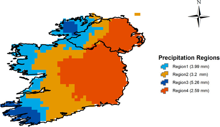
Homogenous regions identified for the Island of Ireland by K‐means clustering of EOBS daily precipitation [Colour figure can be viewed at wileyonlinelibrary.com]
2.3. Derivation of MSLP indices
Two sets of indices were derived from SEAS5 and GloSea5 MSLP hindcasts and used as predictors for precipitation forecasts. The first follows the simple standardized MSLP index of Baker et al. (2018b). The second comprises the three leading components of a rotated empirical orthogonal function (REOF) (Hall and Hanna, 2018; Liu et al., 2019) applied to the ensemble mean MSLP hindcasts from each model and lead time. Figure 2 shows the flowchart of the methodology employed. Further details on the indices are provided below.
FIGURE 2.
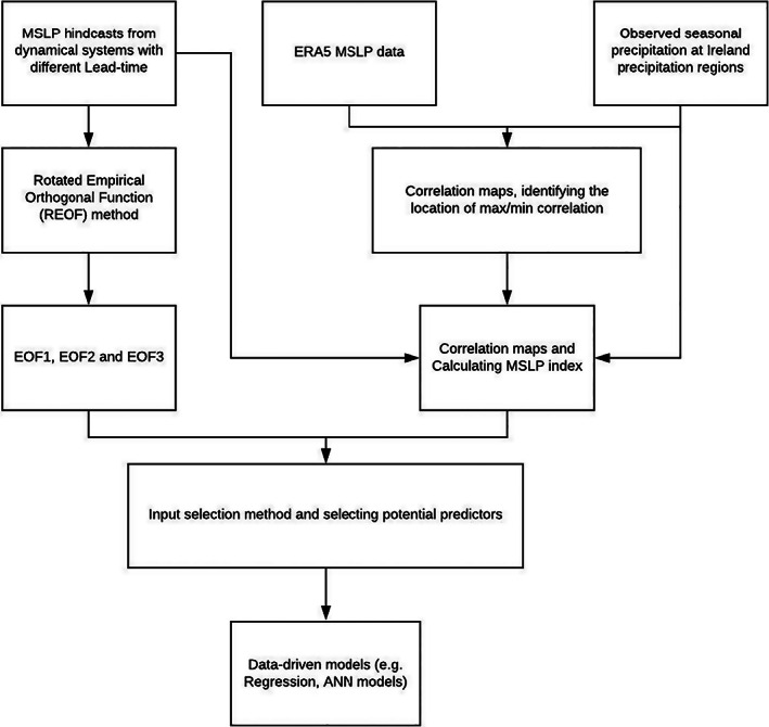
Workflow for the dynamical–statistical approach adopted in this study
2.3.1. Standardized MSLP index
To avoid overfitting real relationships by prescreening predictors directly from model output (DelSole and Shukla, 2009), correlation maps for seasonal mean MSLP from ERA5 versus observed precipitation were first generated for each precipitation region to identify locations of maximum and minimum correlation. We used MSLP with the same spatial domain as Baker et al. (2018b), that is, 50°W–50°E and 20°–80°N. Like Baker et al. (2018b) fixed points of maximum and minimum correlation between MSLP and precipitation from observations are used to derive the standardized MSLP index from model hindcasts for each precipitation region. Depending on the source of the MSLP hindcasts (i.e., GloSea5 or SEAS5), the index is defined as the standardized (i.e., centred about the mean and divided by the standard deviation over the time series) MSLP difference between the fixed maximum and minimum points of correlation from ERA5 MSLP (see Equations (1) and (2)). This index was derived for each precipitation region and lead time separately using the ensemble mean,
| (1) |
| (2) |
where is time (year), is the standardized MSLP from GloSea5 or SEAS5 at the maximum or minimum correlation point (derived from ERA5 MSLP) and and are the mean and standard deviation of MSLP.
2.3.2. Rotated empirical orthogonal equation indices
To derive the EOF indices we applied a REOF as in Hall and Hanna (2018). Rotated EOF analysis can avoid artificial dipole‐type patterns which can be produced by traditional EOF analysis (Lian and Chen, 2012; Liu et al., 2019). Application of REOF to MSLP anomalies was undertaken separately for winter and summer with respect to the long‐term seasonal mean (1993–2016 for GloSea5; 1994–2016 for SEAS5). To account for latitudinal variation in grid cell areas, MSLP anomalies were weighted by the cosine of the latitude prior to analysis. The three leading vectors of the cross‐correlation matrix calculated from monthly MSLP from GloSea5 and SEAS5 hindcasts were used to construct two sets of indices namely , , and , and .
2.4. Empirical models
Using the MSLP indices described above, an exhaustive search was undertaken of every possible combination of predictors when developing our MLR and ANN models. To avoid overfitting, each combination of predictors was tested for collinearity and predictors selected based on adjusted R‐squared (Adj‐R 2 ) which shows the incremental gain in explained variance for every new predictor included. Adj‐R 2 is calculated based on the value of r‐squared, number of independent variables (predictors), and sample size. Predictors were checked for multicollinearity using the variance inflation factor (VIF) and only those with VIF < 4 were retained for further analysis (cf. Lin, 2008).
Models were developed to predict seasonal precipitation up to 4 months in advance, that is, lead‐times (LT) from one to 4 months (henceforth LT1, LT2, LT3, and LT4). We used MSLP hindcasts from both SEAS5 and GloSea5 for lead times of up to 6 months. Therefore, using the average seasonal MSLP derived from monthly MSLP values, the maximum lead‐time which could be provided is 4 months in advance for the first month of each season, followed by 5‐ and 6‐months lead‐time for the second and third months of that season, respectively. As an example, for winter at four‐month lead time (LT4), MSLP is taken as the average of hindcasts from August (i.e., LT4 for December, LT5 for January and LT6 for February). Table S1, Supporting Information shows the various start months used to calculate seasonal precipitation and MSLP with different lead‐times in winter and summer. Model performance was evaluated using the correlation coefficient (r) and mean absolute error (MAE).
2.4.1. Regression models
Multiple linear regression was employed to predict precipitation in different seasons, that is, winter and summer as the target (predictand) with selected MSLP indices from hindcasts as predictors. Regression models were built for each season, lead time, and region (i.e., 2 seasons × 4 lead‐times × 5 regions, yielding 40 models). Using selected predictors, regression models were fitted using leave‐one‐out cross‐validation (LOOCV). In this method, first 1 year is left out and the model is calibrated based on data in other years and the error associated with prediction (of the year omitted from calibration) is recorded. This procedure is repeated for all years and the overall prediction error is computed as the average of all test error estimates.
2.4.2. Artificial neural network
A multilayer perceptron neural network with two hidden layers, trained by backpropagation, was used as the second model for precipitation prediction. The same predictors identified for the MLR method for each region, season and lead time were used. Logistic and linear activation functions were employed for training hidden and output layers, respectively. The optimum number of neurons in each hidden layer was identified via trial‐and‐error. Again, a separate ANN model was built for each season, lead time, and region. Figure S1 shows an example ANN architecture for the case of winter precipitation at LT3 using , , and as the best inputs. Two hidden layers were employed, comprising two neurons for the first hidden‐layer and three for the second. The performance of the ANN model was also assessed using the LOOCV method.
2.4.3. Benchmark models
To evaluate the added skill of the new methods, we apply a zero‐order forecast (ZOF) based on the persistence of observed precipitation (following Dixon and Wilby, 2016). This method assumes that the precipitation at time is the same as at time (i.e., the previous time step). In addition, the ensemble mean precipitation hindcasts from GloSea5 and SEAS5 for each lead time were first averaged over each precipitation region in Figure 1, then bias‐corrected via empirical quantile mapping (Cannon et al., 2015). The results were then compared with precipitation derived from the developed models over those regions. Finally, we derived a climatology benchmark from EOBS for each region using a moving average method. In this case, for each prediction year, the mean precipitation based on a subset of data with length (window size) up to that year () is considered as the predicted precipitation value for that year. Then this averaging window is shifted forward by 1 year to calculate the predicted value at year . We evaluated different window sizes ranging from 5 to 30 years to determine the optimum (i.e., toughest to beat) climatology benchmark based on MAE.
2.5. Uncertainty analysis
Having identified the model with most satisfactory performance for each rainfall region, season, and lead time, an uncertainty analysis was conducted using different combinations of input–output data for training–testing the regression and ANN models. This provides an estimate of uncertainty associated with the sampling period, that is, due to climate variability. It should be noted that this does not capture uncertainty among dynamical model ensembles members (because we only consider the ensemble mean as in Baker et al., 2018b), nor uncertainties associated with the prediction models themselves, that is, from fitted coefficients of the regression model or the weights of the ANN (see section 4). One thousand random combinations of input–output data were selected to train/test the statistical models for each region‐lead‐time‐season and the resultant forecasted precipitation time series was used to derive 95% confidence intervals of predictions (2.5 and 97.5% percentiles), and to calculate the precipitation with 50% likelihood. Next, p‐ and r‐factors were used to evaluate model performance. The p‐factor shows the percentage of observed data bracketed by the 95% uncertainty range. The closer to 1, the better the model performance. The r‐factor evaluates the width of the uncertainty band and is calculated using the following equations:
| (3) |
where is the standard deviation of variable (observed precipitation) and is calculated using following equation:
| (4) |
where is number of observed data, and are upper (97.5%) and lower (2.5%) boundaries of uncertainty band. Again, an value closer to 1 is desirable (Abbaspour, 2008).
3. RESULTS
3.1. Correlation analysis
The correlation between MSLP and precipitation was found to be similar between regions, but varies by lead time and season and also depends on the dynamical model. Figure 3 shows example correlation surfaces for observed winter and summer precipitation versus MSLP with 1‐month lead‐time from GloSea5 for Regions 3 and 4 as the wettest and driest regions, respectively. Figure 4 shows the same information but for SEAS5. Plus signs denote the locations of maximum and minimum correlation values for each case based on observed MSLP from ERA5. The correlation patterns for GloSea5 and SEAS5 are most similar in winter for LT = 1 (Figures 3a,b and 4a,b) but differ in summer (Figures 3c,d and 4c,d). The MSLP values at maximum and minimum correlation points on each map were used to calculate the standardized MSLP‐based indices for each lead‐time and region. Table S2 shows the correlation ranges obtained for GloSea5 and SEAS5 derived from standardized MSLP indices and precipitation across all regions, lead times, and seasons. The leading EOF patterns derived from GloSea5 and SEAS5 for the different seasons and 1‐month lead‐time are shown in Figures S4–S7, respectively.
FIGURE 3.
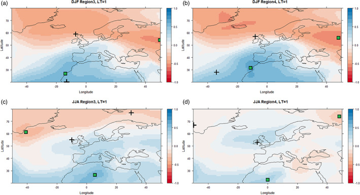
Correlation surfaces for winter (DJF) MSLP with 1‐month lead‐time and winter precipitation (a, b) and summer (JJA) MSLP with 1‐month lead‐time and summer precipitation (c, d) based on GloSea5 for the period 1994–2016 for Regions 3 and 4. Crosses show the location of maximum and minimum correlation values in each case calculated using the ERA5 MSLP dataset. Green squares show the location of max/min correlation between models and observations (GloSea5 MSLP v E‐OBS precipitation) [Colour figure can be viewed at wileyonlinelibrary.com]
FIGURE 4.
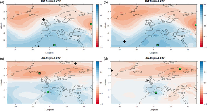
As in Figure 3 but for MSLP from SEAS5 [Colour figure can be viewed at wileyonlinelibrary.com]
Correlation analysis between standardized MSLP indices/EOFs and observed precipitation over each season, lead‐time, region, and MSLP product was performed to assess how well those potential predictors are related to observed precipitation. The results are shown in Figure 5. For all regions in winter, and EOF3 from GloSea5 have significant (p = .05) positive and negative correlations with winter precipitation, respectively and are considered as potential predictors for regression models for 1‐month lead‐time. For the 2‐month lead‐time in winter, the strongest correlations between observed precipitation in each region are for EOF3 from SEAS5 (r < −0.39 for all regions) and for EOF2 from GloSea5 (r > 0.33), respectively. For 3‐month lead‐time in winter, EOF1 (r < −0.42) and EOF3 (r < −0.39) from SEAS5 show significant negative correlations and are, therefore, candidates for precipitation prediction over all regions, together with EOF2 from GloSea5 (r > 0.30). For LT4, the strongest positive and negative significant correlations are evident for EOF3 from GloSea5 and EOF2 from SEAS5, respectively.
FIGURE 5.
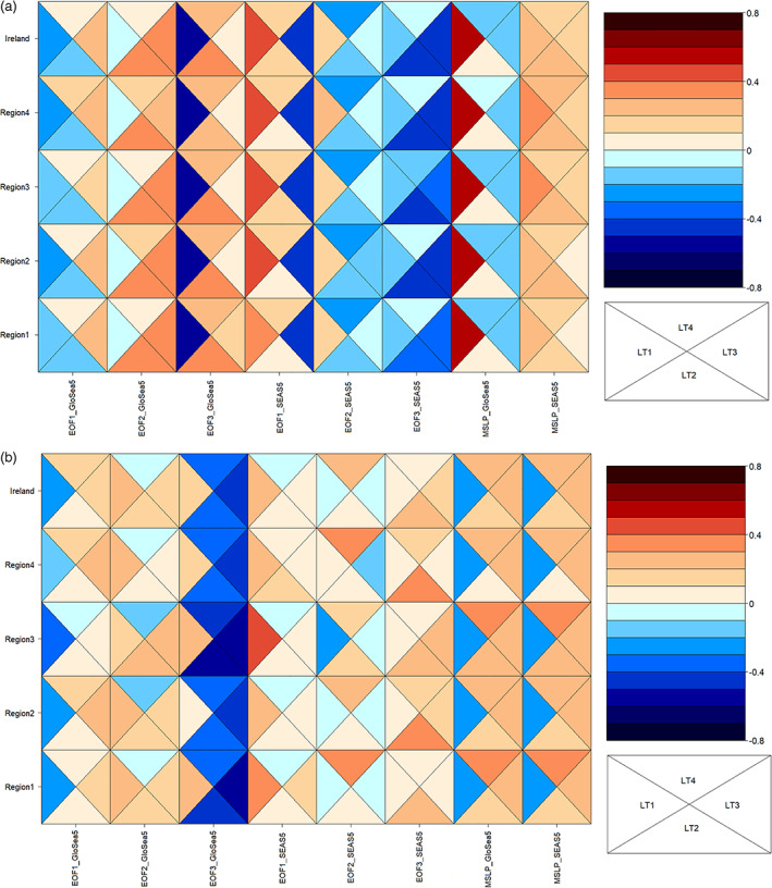
Correlations between dynamical model MSLP EOF indices and precipitation by lead time (LT) and region in (a) winter and (b) summer [Colour figure can be viewed at wileyonlinelibrary.com]
Summer correlations show greater variation by lead time and between regions (Figure 5b). For some lead‐times, multiple highly correlated indices which could be a promising predictor for most regions are evident but at other lead‐times few predictors with significant correlation with precipitation are found. For 1‐month lead‐time, EOF1 from GloSea5 (r < −0.18), (r < −0.23) and (r < −0.23) show significant negative correlations and are potential predictors for statistical models in all regions. For the 2‐month lead‐time, EOF3 from GloSea5 has the strongest negative correlation with summer precipitation over all regions (r > −0.33), while EOF3 from SEAS5 showed the strongest significant positive correlations (r > 0.22) among all signals. For the 3‐month lead‐time, again EOF3 from GloSea5 (r < −0.43) and and can be used as a potential predictor for all regions. Finally, for the 4‐month lead‐time, EOF3 from GloSea5 for all regions (r < −0.34) and and may be useful candidates for statistical models to predict summer precipitation, returning statistically significant correlations at 5% significance level.
Previous research (e.g., Moore et al., 2013; Tošić et al., 2014), found that EOF1 is associated with the NAO in both winter and summer, whereas EOF2 represents the East Atlantic (EA) pattern which is more prominent in winter, comprising a north–south dipole of anomalies. The EA pattern resembles the NAO, but with pressure anomaly centres displaced southeastward and thus is sometimes interpreted as a “southward shifted” NAO (Barnston and Livezey, 1987). Some EOFs derived from the MSLP hindcasts of GloSea5 and SEAS5 do not show physical resemblance to associated climate signals, that is, NAO or EA. It has previously been observed that when different MSLP datasets are used, and due to the constraining (orthogonal) nature of the EOF analysis, patterns may vary markedly between models (Walz et al., 2018). Moreover, in similar studies in which EOFs are connected to large climate signals, long‐term sea level pressure data have been used (e.g., MSLP data from 1925 to 1977 (Trenberth and Paolino Jr, 1981); 1900–2010 (Parker et al., 2019)). We used MSLP hindcast from 1994 to 2016 which might lead to different patterns or displacement of centres of action. Also using the ensemble mean can lead to differences as the observed EOFs contain unpredictable as well as predictable components. This might be another reason for absence of physically interpretable EOFs in some cases.
3.2. Forecast performance
To assess the added value of using EOFs in our analyses, two sets of potential predictors are considered when developing empirical models. First, only MSLP‐based indices are used as input to the models. Second, we used all potential predictors including MSLP‐based and EOFs from GloSea5 and SEAS5 (Figures S8 and S9). An exhaustive search method was employed to identify the best combination of predictors for each region and lead‐time based on all predictors with significant correlation with precipitation. Evidently, utilizing EOFs alongside MSLP‐based indices does improve forecast skill in most regions and lead‐times (Figure S8). Consequently, we retain all potential predictors. Table 1 summarizes the selected predictors for each model (i.e., by region, season, and lead‐time). EOFs from SEAS5 were selected as predictors in data‐driven models for most regions, lead‐times, and seasons. The optimum architecture identified for each ANN is presented in Table S3. A sensitivity analysis of the length of moving average window for the climatology benchmark (Figure S10) determined that a 30‐year window minimizes MAE in both summer and winter across all regions and was thus employed.
TABLE 1.
The predictors selected for regression and ANN models by lead time (LT), season, and region
| Lead‐time | ||||||
|---|---|---|---|---|---|---|
| LT = 1 | LT = 2 | LT = 3 | LT = 4 | |||
| Winter | Region1 | + + | + | + | + | |
| Region2 | + + + | + + | + + + + | + | ||
| Region3 | + + + | + | + + | + | ||
| Region4 | + + + |
|
+ + + + | + | ||
| Ireland | + + |
|
+ + | + | ||
| Summer | Region1 |
|
+ + + | + + + + | + + + + | |
| Region2 | + | + + + | + + + + | + + + + | ||
| Region3 | + + | + + + + | + + + + | + + + | ||
| Region4 | + + + | + | + + + | + + + | ||
| Ireland | + | + + + + + | + + + + | + + + + + | ||
Hindcasts for winter and summer precipitation with 1‐month lead‐time are presented in Figures 6 and 7. Overall, for both seasons, regression and ANN hindcasts outperform the persistence, climatology, and bias‐corrected dynamical model output for all regions. Moreover, at the 1‐month lead‐time, the ANN and MLR show some skill at predicting extreme seasons. For example, the dry summer of 1995 and wettest winter on record 2015/2016 are captured well by our hybrid models. Scaife et al. (2017) show that the intensified cyclonic flow over the Atlantic in winter 2015/2016 were well predicted by the GloSea5 system. However, the extremeness of the wet 2013/2014 winter and sequence of exceptionally wet summers in 2007–2009 are underestimated (Matthews et al., 2014; 2016; Noone et al., 2016). Knight et al. (2017) assert that the tropics played a significant role in the development of the unusual extratropical circulation that led to widespread high precipitation over the UK in winter 2013–2014.
FIGURE 6.
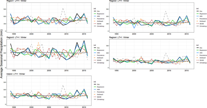
Winter precipitation hindcasted for each region for LT1. Results are shown for EOBS observations (black line), the MLR (green), the ANN (blue), persistence (grey dashed), bias corrected GloSea5 (orange), SEAS5 (red) and climatology (grey) precipitation [Colour figure can be viewed at wileyonlinelibrary.com]
FIGURE 7.
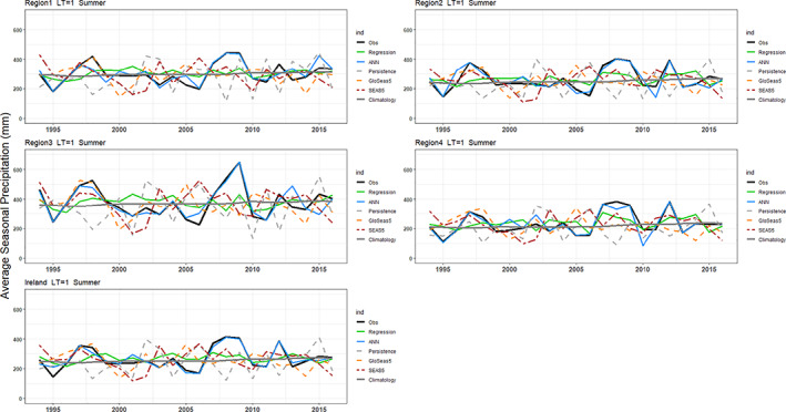
As in Figure 6 but for summer [Colour figure can be viewed at wileyonlinelibrary.com]
Performance criteria (i.e., CC and MAE) derived from the different hindcasts across seasons, lead‐times, and regions are shown in Figure 8. For MAE, both the ANN and regression models have the best performance (Figure 8) in winter for all lead‐times compared with other benchmark methods; the ANN outperforms regression at most lead‐times over most regions except LT1 in winter. In this case, the average MAE for all regions is 88 mm for the ANN model, compared with MAE of 85 mm for the MLR model. Except for SEAS5 precipitation in winter for LT3, climatology is the next best performing alterative to the ANN/MLR models. MAE results again show that the persistence method followed by SEAS5 yield the worst performance in winter at lead‐times 1 and 4 and GloSea5 for most regions at lead‐times 2 and 3. In summer, the persistence method followed by SEAS5 has the worst performance in most cases, except at lead‐time 2 where SEAS5 performs worse than the persistence method (Figure 8). It can also be seen that all hindcasts have slightly better performance for Region 4 (driest region) and the weakest performance over Region 3 (wettest region).
FIGURE 8.
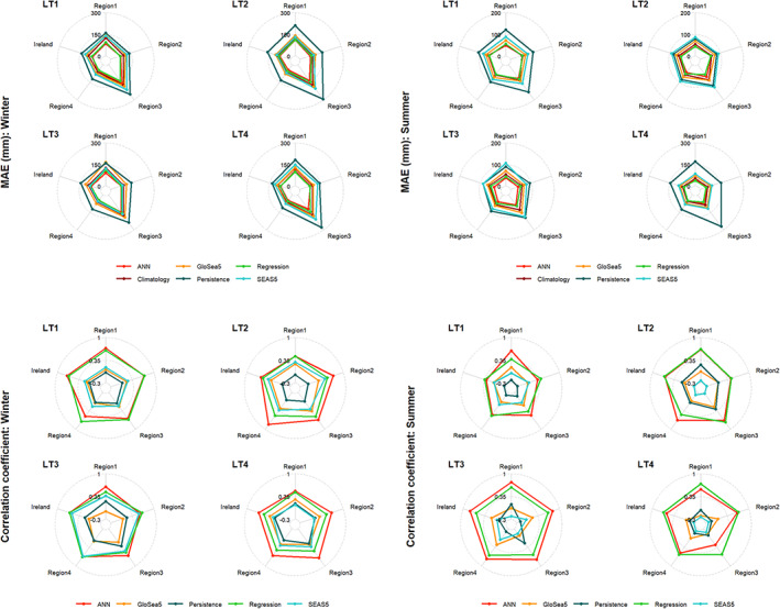
Performance of the methods as evaluated using MAE, and correlation coefficient for different lead‐times (LT) and regions in winter (left column) and summer (right column) [Colour figure can be viewed at wileyonlinelibrary.com]
Based on the correlation coefficient, again ANN and MLR have most skilful hindcasts for all lead‐times, regions, and seasons with average correlation values of 0.59 and 0.58 for the ANN and 0.50 and 0.56 for MLR in winter and summer, respectively (Figures 8 and S11). The ANN has superior performance in both winter and summer except for LT1 in winter and LT4 in summer; for LT1 and LT2 in summer the ANN and MLR models have very similar performance. In winter, bias‐corrected precipitation from SEAS5 has higher correlation with observations compared to the equivalent from GloSea5 for LT1 and LT3. At LT4, precipitation from GloSea5 performs slightly better over Regions 1 and 2 and Ireland. In summer, the persistence method has higher correlation than GloSea5 and SEAS5 precipitation for LT2.
In summary, our new dynamical–statistical methods perform satisfactorily in prediction of precipitation up to 4 months ahead, surpassing all available benchmarks in both winter and summer. The ANN performs better than MLR in most regions in summer especially for LT1 and LT3, and in winter for LT2, LT3 and LT4. However, the MLR marginally outperforms ANN in most regions at LT1 in winter and LT4 in summer (Figure S11). The skill of bias‐corrected precipitation forecasts from SEAS5 and GloSea5 are generally not as good as climatology in winter and only marginally better than persistence in summer for some lead‐times/regions. For example, the correlations between bias‐corrected SEAS5 and GloSea5 and observed precipitation are −0.001 and 0.06 in winter, and 0.06 and 0.03 in summer, respectively.
To test whether the choice of predictors influences skill over different regions, we generalized the predictors selected for the Island of Ireland to other regions, that is, used identical predictors for all regions. The results are shown in Figure S12 in terms of the correlation coefficient. Using fixed predictors for all regions marginally increases skill in some cases (e.g., ANN in LT1 and ANN and MLR methods in LT4), makes no difference in others (e.g., MLR at LT2 and ANN and MLR methods at LT3) or, in a few cases, decreases the correlation coefficient (e.g., MLR at LT1 over Regions 2, 3, and 4). Based on these results there is no obvious evidence to suggest any systemic overfitting.
3.3. Uncertainty analysis
Given the consistently strong performance of the ANN method across regions, lead‐times, and seasons, uncertainty due to sampling of calibration period was evaluated by applying different combinations of train‐test periods as input to the ANN. For illustrative purposes, Figures 9 and 10 show 95% confidence intervals (grey area), with the median modelled precipitation (red dashed‐line) and observed precipitation (black line) for different regions and seasons at LT1. It is noteworthy that when varying the calibration period, hindcasts are more successful at capturing extreme seasons. Moreover, the wettest winters (including 2013/14 and 2015/16) are better captured by hindcasts at LT1 and LT3 than other lead‐times. Table 2 shows the and values for each region and lead‐time. Sampling uncertainty associated with ANN model forecasts is greater in summer for all lead‐times (i.e., there are larger r‐factors in summer compared to winter). However, the uncertainty band brackets more observed precipitation in summer than winter (as shown by the p‐factors) for most lead‐times and regions. Although all regions have less uncertainty in winter than summer, more of the observations lie within the uncertainty band of the LT1 forecast (i.e., greater p‐factor in winter compared to summer) in Regions 2 and 3 and Ireland. For LT2, the uncertainty in winter is less than summer while a higher proportion of the observations are bracketed by the 95% uncertainty band in summer compared to winter, except in Region 3. Finally, for LT4, sampling uncertainty associated with summer is greater than winter, while more data are bracketed by the uncertainty band in summer in all regions.
FIGURE 9.
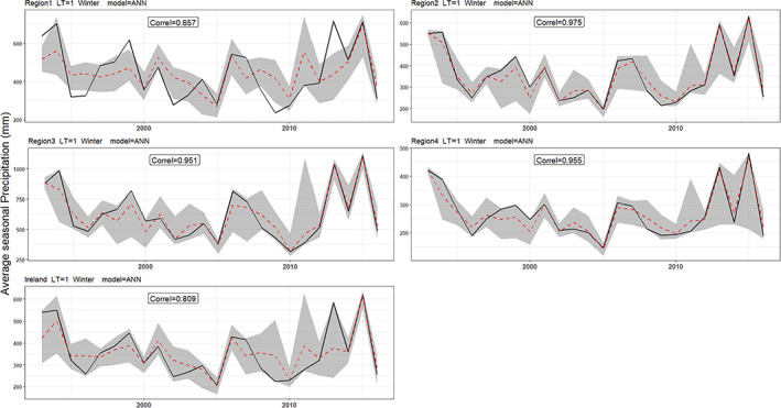
ANN model results for different regions with LT = 1 month in winter, showing the 95% uncertainty band (grey shaded area), the median forecast (red dashed line) and observed precipitation (black line) [Colour figure can be viewed at wileyonlinelibrary.com]
FIGURE 10.
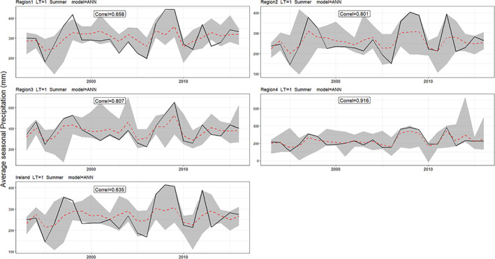
As in Figure 9, but for summer [Colour figure can be viewed at wileyonlinelibrary.com]
TABLE 2.
Summary of r‐ and p‐factors associated with the uncertainty in application of the ANN model for each lead time (LT), region and season
| Region | Winter | Summer | |||||||
|---|---|---|---|---|---|---|---|---|---|
| LT1 | LT2 | LT3 | LT4 | LT1 | LT2 | LT3 | LT4 | ||
| r‐factor | Region1 | 1.05 | 1.21 | 1.48 | 1.13 | 1.41 | 1.94 | 1.96 | 1.92 |
| Region2 | 0.96 | 0.87 | 1.04 | 0.99 | 1.67 | 2.51 | 1.98 | 1.64 | |
| Region3 | 1.07 | 1.43 | 1.37 | 0.95 | 1.97 | 1.71 | 1.82 | 2.14 | |
| Region4 | 1.07 | 0.82 | 1.19 | 0.76 | 2.65 | 1.85 | 2.05 | 1.63 | |
| Ireland | 1.18 | 0.91 | 1.33 | 0.93 | 1.49 | 2.54 | 2.03 | 1.92 | |
| p‐factor | Region1 | 0.59 | 0.88 | 0.99 | 0.75 | 0.79 | 0.92 | 1 | 1 |
| Region2 | 0.99 | 0.51 | 0.99 | 0.71 | 0.83 | 1 | 1 | 1 | |
| Region3 | 0.98 | 0.99 | 0.99 | 0.76 | 0.96 | 0.88 | 0.96 | 1 | |
| Region4 | 0.96 | 0.38 | 0.96 | 0.58 | 1 | 0.96 | 1 | 1 | |
| Ireland | 0.92 | 0.55 | 0.96 | 0.77 | 0.75 | 1 | 1 | 1 | |
4. DISCUSSION AND CONCLUSION
We developed hybrid dynamical–statistical approaches to seasonal forecasting of winter and summer precipitation for Ireland over lead times of 1–4 months using hindcasts of MSLP from two dynamical forecasting systems (SEAS5 and GloSea5). We used MLR and ANNs to relate MSLP to observed precipitation over four distinct rainfall regions as well as averaged across the Island of Ireland as a whole. MSLP hindcasts from SEAS5 and GloSEA5 were postprocessed in two ways before being used as potential predictors in our statistical modelling approach. First, we identified the locations of grids with most positive and negative correlations based on ERA5 MSLP (over the period 1993/1994–2016) when correlated with observed (EOBS) precipitation for each region and season. Next, standardized indices of MSLP anomalies were derived from hindcasts of MSLP from dynamical models using the same fixed max/min points of correlation specified for each precipitation region, season, and lead‐time. Second, we deployed REOF analysis to hindcasts of MSLP from SEAS5 and GloSea5 to identify the three leading components for each forecast horizon. We evaluated the performance of this dynamical–statistical approach against bias‐corrected precipitation forecasts from SEAS5 and GloSea5, all benchmarked against skill from persistence and climatology alone.
As with Baker et al. (2018b), we find that our dynamical–statistical approach improves forecast skill relative to bias‐corrected, dynamical forecast system output. Our ANN and MLR approaches provide greatest skill for all lead times and regions in both summer and winter; they also outperform precipitation from dynamical models, climatology, and persistence. Consistent with Nobakht et al. (2021), precipitation forecasts from SEAS5 performed marginally better than GloSea5, except for LT4 in winter over Regions 1 and 2. Although we used a relatively simple bias correction method, future research might achieve greater accuracy via more sophisticated post‐processing methods, such as quantile delta mapping (Cannon et al., 2015; Mendez et al., 2020).
Among the potential predictors available, those based on standardized MSLP showed strongest correlations (spanning 0.35–0.63) with precipitation across both seasons, all lead times and regions. This highlights that indices based on MSLP provide a reliable basis for forecasting precipitation over the Island of Ireland, especially in winter. MLSP might also enhance seasonal forecast skill for other climate variables and regions where there is covariance with precipitation, such as for atmospheric humidity, air temperature, sunshine hours and wind speeds (e.g., Hillier et al., 2020).
Interestingly, some of the strongest correlations were found between summer precipitation and EOF3 from GloSea5 data (), with this index selected as a predictor for many regions/lead‐times. This EOF is usually interpreted as the East Atlantic (EA) pattern (Hall and Hanna, 2018), and has also been used in some weather generators as a predictor variable (ATKINS, 2020). Hence, although the NAO has long been recognized as a major driver of climate variability in Northwest Europe, we note that an apparent EA pattern emerges as a key signal of summertime predictability in the dynamical models. EOF3 from SEAS5 also showed strong negative correlation with precipitation in most regions in winter. However, while for some lead‐times the EOFs from GloSea5 and SEAS5 are physically interpretable (e.g., EOF1 from GloSea5 in winter and EOF1 from SEAS5 in summer are both similar to NAO), others are not physically interpretable. For example summer EOF3 from GloSea5 is somewhat similar to Scandinavian pattern (SCA) but the negative centre has a more northeasterly position. Undoubtedly, the physical interpretability is hampered by the brevity of available hindcast MSLP data. Moreover, the MSLP data used for EOF analysis are raw hindcasts from dynamical models, not observations. We also used the ensemble mean rather than ensemble members which could further explain the unfamiliar EOF patterns.
The dynamical–statistical approach developed here leverages two forecasting systems to develop prototype predictions of winter and summer precipitation with up to 4 months lead for regions across the Island of Ireland. Our ANN and regression models show the most consistently better results compared with bias corrected dynamical outputs, climatology, and persistence methods. The possibility of model overfitting was reduced by applying leave‐one‐out cross validation, use of adjusted R‐square when evaluating different sets of predictors, as well as use of a smaller set of predictors in all models (Figure S12). Although our dynamical–statistical models performed well in both winter and summer, the ANN provided marginally higher skill in winter, and the MLR in summer. Whereas the ANN and MLR models revealed variability in skill for the wettest rainfall regions in winter and the driest in summer, the MLR model returned most skilful and consistent results in summer for LT1, LT2, and LT4 with average correlation scores of 0.39, 0.59, and 0.64, respectively. However, the ANN model achieved more skilful and consistent results in winter across most regions and lead times, with an average correlation coefficient of 0.61 over all regions for LT1. In comparison, Baker et al. (2018b) obtained correlations up to 0.70 between regression‐based hindcasts and observed precipitation in winter for the UK. The encouraging performance of these models, particularly in summer, is noteworthy and paves the way to improved drought forecasting in summer and winter. Previous studies in the region have primarily focused on winter predictions (e.g., Scaife et al., 2014; Baker et al., 2018b; Stringer et al., 2020) or the evaluation of predictors that could be used for summer precipitation/temperature forecasts but without evaluating predictive skill in summer (e.g., Fowler and Kilsby, 2002). Also as Knight et al. (2017) reported a significant role of tropical circulation in high precipitation totals over the UK, for example, in winter 2013–2014, in future studies the domain to explore MSLP might be expanded to include tropical regions. Finally, as the availability of hindcasts increases future work may also further assess model performances using out of sample tests for more recent years.
Our findings demonstrate the feasibility of skilful seasonal forecasts of winter and summer precipitation in Ireland. Such forecasts could be of value to many sectors, not least the water industry. However, before evaluating their operational utility, future work should extend the analysis of uncertainty presented here. For example, individual ensemble members rather than just the ensemble mean could be used to generate probabilistic seasonal forecasts. The uncertainty analysis framework used here evaluated uncertainties due to climate variability but not from the dynamical model ensembles. In addition, uncertainties from the statistical models themselves (i.e., the uncertainty in fitted coefficients of regression model and weights of the ANN) were not included. Moreover, predictor–predictand relationships were treated as stationary in this research; for operational purposes the ANN/regression models should be re‐calibrated using a moving window to capture any evolution in the relationships. There is also the possibility of assessing other candidate predictors and domains in future work. For instance, bias‐corrected precipitation forecasts from dynamical systems could be used as inputs to data‐driven models alongside the MSLP‐based indices employed here.
AUTHOR CONTRIBUTIONS
Saeed Golian: Conceptualization; formal analysis; methodology; software; supervision; validation; visualization; writing – original draft; writing – review and editing. Conor Murphy: Conceptualization; methodology; project administration; supervision; validation; writing – review and editing. Robert L. Wilby: Methodology; validation; writing – review and editing. Tom Matthews: Methodology; validation; writing – review and editing. Seán Donegan: Data curation; writing – review and editing. Dáire Foran Quinn: Data curation; resources. Shaun Harrigan: Methodology; validation; writing – review and editing.
Supporting information
Appendix S1: Supporting information
ACKNOWLEDGEMENTS
This research was funded through a Science Foundation Ireland Career Development Award to CM (Grant/Award No. SFI/17/CDA/4783). Open access funding provided by IReL. [Correction added on 20 May 2022, after first online publication: IReL funding statement has been added.]
Golian, S. , Murphy, C. , Wilby, R. L. , Matthews, T. , Donegan, S. , Quinn, D. F. , & Harrigan, S. (2022). Dynamical–statistical seasonal forecasts of winter and summer precipitation for the Island of Ireland. International Journal of Climatology, 42(11), 5714–5731. 10.1002/joc.7557
Funding information Science Foundation Ireland, Grant/Award Number: SFI/17/CDA/4783
REFERENCES
- Abbaspour, K.C. (2008) SWAT‐CUP: SWAT calibration and uncertainty programs—a user manual (pp. 16–70). Dübendorf, Switzerland: Eawag. [Google Scholar]
- Agrawala, S. , Broad, K. and Guston, D.H. (2001) Integrating climate forecasts and societal decision making: challenges to an emergent boundary organization. Science, Technology, & Human Values, 26(4), 454–477. [Google Scholar]
- Al Samouly, A. , Luong, C.N. , Li, Z. , Smith, S. , Baetz, B. and Ghaith, M. (2018) Performance of multi‐model ensembles for the simulation of temperature variability over Ontario, Canada. Environmental Earth Sciences, 77(13), 1–12. [Google Scholar]
- ATKINS . (2020) Regional climate data tools. Final report. Available at: https://www.wrse.org.uk/media/ok1mtsoq/wrse_file_1338_regional-climate-data-tools.pdf.
- Baker, L.H. , Shaffrey, L.C. and Scaife, A.A. (2018b) Improved seasonal prediction of UK regional precipitation using atmospheric circulation. International Journal of Climatology, 38, e437–e453. [Google Scholar]
- Baker, L.H. , Shaffrey, L.C. , Sutton, R.T. , Weisheimer, A. and Scaife, A.A. (2018a) An intercomparison of skill and overconfidence/underconfidence of the wintertime North Atlantic Oscillation in multimodel seasonal forecasts. Geophysical Research Letters, 45(15), 7808–7817. [Google Scholar]
- Barnston, A.G. and Livezey, R.E. (1987) Classification, seasonality and persistence of low‐frequency atmospheric circulation patterns. Monthly Weather Review, 115(6), 1083–1126. [Google Scholar]
- Bell, V.A. , Davies, H.N. , Kay, A.L. , Brookshaw, A. and Scaife, A.A. (2017) A national‐scale seasonal hydrological forecast system: development and evaluation over Britain. Hydrology and Earth System Sciences, 21(9), 4681–4691. [Google Scholar]
- Cannon, A.J. , Sobie, S.R. and Murdock, T.Q. (2015) Bias correction of GCM precipitation by quantile mapping: How well do methods preserve changes in quantiles and extremes? Journal of Climate, 28(17), 6938–6959. [Google Scholar]
- Ceglar, A. and Toreti, A. (2021) Seasonal climate forecast can inform the European agricultural sector well in advance of harvesting. Npj Climate and Atmospheric Science, 4(1), 1–8. [Google Scholar]
- Clark, R.T. , Bett, P.E. , Thornton, H.E. and Scaife, A.A. (2017) Skilful seasonal predictions for the European energy industry. Environmental Research Letters, 12(2), 024002. [Google Scholar]
- Comas‐Bru, L. and McDermott, F. (2014) Impacts of the EA and SCA patterns on the European twentieth century NAO–winter climate relationship. Quarterly Journal of the Royal Meteorological Society, 140(679), 354–363. [Google Scholar]
- Cornes, R.C. , van der Schrier, G. , van den Besselaar, E.J. and Jones, P.D. (2018) An ensemble version of the E‐OBS temperature and precipitation data sets. Journal of Geophysical Research: Atmospheres, 123(17), 9391–9409. [Google Scholar]
- Crhová, L. and Holtanová, E. (2018) Simulated relationship between air temperature and precipitation over Europe: sensitivity to the choice of RCM and GCM. International Journal of Climatology, 38(3), 1595–1604. [Google Scholar]
- da Paz, A.R. , Uvo, C. , Bravo, J. , Collischonn, W. and da Rocha, H.R. (2011) Seasonal precipitation forecast based on artificial neural networks. In: Computational Methods for Agricultural Research: Advances and Applications. IGI Global, pp. 326–354. [Google Scholar]
- DelSole, T. and Shukla, J. (2009) Artificial skill due to predictor screening. Journal of Climate, 22(2), 331–345. [Google Scholar]
- Devi, U. , Shekhar, M.S. , Singh, G.P. and Dash, S.K. (2020) Statistical method of forecasting of seasonal precipitation over the Northwest Himalayas: North Atlantic Oscillation as precursor. Pure and Applied Geophysics, 177, 1–11. [Google Scholar]
- Ding, T. and Ke, Z. (2013) A comparison of statistical approaches for seasonal precipitation prediction in Pakistan. Weather and Forecasting, 28(5), 1116–1132. [Google Scholar]
- Dixon, S.G. and Wilby, R.L. (2016) Forecasting reservoir inflows using remotely sensed precipitation estimates: a pilot study for the River Naryn, Kyrgyzstan. Hydrological Sciences Journal, 61(1), 107–122. [Google Scholar]
- Doblas‐Reyes, F.J. , Hagedorn, R. and Palmer, T.N. (2006) Developments in dynamical seasonal forecasting relevant to agricultural management. Climate Research, 33(1), 19–26. [Google Scholar]
- Donegan, S. , Murphy, C. , Harrigan, S. , Broderick, C. , Foran Quinn, D. , Golian, S. , Knight, J. , Matthews, T. , Prudhomme, C. , Scaife, A.A. and Stringer, N. (2021) Conditioning ensemble streamflow prediction with the North Atlantic Oscillation improves skill at longer lead times. Hydrology and Earth System Sciences, 25(7), 4159–4183. [Google Scholar]
- Dunstone, N. , Smith, D. , Scaife, A. , Hermanson, L. , Fereday, D. , O'Reilly, C. , Stirling, A. , Eade, R. , Gordon, M. , MacLachlan, C. and Woollings, T. (2018) Skilful seasonal predictions of summer European rainfall. Geophysical Research Letters, 45(7), 3246–3254. [Google Scholar]
- ECMWF . (2019) Seasonal forecasts and the copernicus climate change service. Available at: https://confluence.ecmwf.int/display/CKB/Seasonal+forecasts+and+the+Copernicus+Climate+Change+Service.
- Emerton, R. , Zsoter, E. , Arnal, L. , Cloke, H.L. , Muraro, D. , Prudhomme, C. , Stephens, E.M. , Salamon, P. and Pappenberger, F. (2018) Developing a global operational seasonal hydro‐meteorological forecasting system: GloFAS‐Seasonal v1. 0. Geoscientific Model Development, 11(8), 3327–3346. [Google Scholar]
- Folland, C.K. , Knight, J. , Linderholm, H.W. , Fereday, D. , Ineson, S. and Hurrell, J.W. (2009) The summer North Atlantic Oscillation: past, present, and future. Journal of Climate, 22(5), 1082–1103. [Google Scholar]
- Foran Quinn, D. , Murphy, C. , Wilby, R.L. , Matthews, T. , Broderick, C. , Golian, S. , Donegan, S. & Harrigan, S. (2021) Benchmarking seasonal forecasting skill using river flow persistence in Irish catchments. Hydrological Sciences Journal, 66(4), 672–688. [Google Scholar]
- Fowler, H.J. and Kilsby, C.G. (2002) Precipitation and the North Atlantic Oscillation: a study of climatic variability in northern England. International Journal of Climatology, 22(7), 843–866. [Google Scholar]
- Gubler, S. , Sedlmeier, K. , Bhend, J. , Avalos, G. , Coelho, C.A.S. , Escajadillo, Y. , Jacques‐Coper, M. , Martinez, R. , Schwierz, C. , De Skansi, M. and Spirig, C. (2020) Assessment of ECMWF SEAS5 seasonal forecast performance over South America. Weather and Forecasting, 35(2), 561–584. [Google Scholar]
- Hall, R.J. and Hanna, E. (2018) North Atlantic circulation indices: links with summer and winter UK temperature and precipitation and implications for seasonal forecasting. International Journal of Climatology, 38, e660–e677. [Google Scholar]
- Hall, R.J. , Scaife, A.A. , Hanna, E. , Jones, J.M. and Erdélyi, R. (2017) Simple statistical probabilistic forecasts of the winter NAO. Weather and Forecasting, 32(4), 1585–1601. [Google Scholar]
- Hameed, S. and Riaz, S.M. (2020) Impact of the Icelandic Low on British climate in winter. International Journal of Climatology., 40, 6337–6345. [Google Scholar]
- Hersbach, H. , Bell, B. , Berrisford, P. , Hirahara, S. , Horányi, A. , Muñoz‐Sabater, J. , Nicolas, J. , Peubey, C. , Radu, R. , Schepers, D. and Simmons, A. (2020) The ERA5 global reanalysis. Quarterly Journal of the Royal Meteorological Society, 146(730), 1999–2049. [Google Scholar]
- Hewitt, C. , Buontempo, C. and Newton, P. (2013) Using climate predictions to better serve society's needs. Eos, Transactions American Geophysical Union, 94(11), 105–107. [Google Scholar]
- Hillier, J.K. , Matthews, T. , Wilby, R.L. and Murphy, C. (2020) Multi‐hazard dependencies can increase or decrease risk. Nature Climate Change, 10(7), 595–598. [Google Scholar]
- Hurrell, J.W. and Deser, C. (2010) North Atlantic climate variability: the role of the North Atlantic Oscillation. Journal of Marine Systems, 79(3–4), 231–244. [Google Scholar]
- Johnson, S.J. , Stockdale, T.N. , Ferranti, L. , Balmaseda, M.A. , Molteni, F. , Magnusson, L. , Tietsche, S. , Decremer, D. , Weisheimer, A. , Balsamo, G. and Keeley, S.P. (2019) SEAS5: the new ECMWF seasonal forecast system. Geoscientific Model Development, 12(3), 1087–1117. [Google Scholar]
- Knight, J.R. , Maidens, A. , Watson, P.A. , Andrews, M. , Belcher, S. , Brunet, G. , Fereday, D. , Folland, C.K. , Scaife, A.A. and Slingo, J. (2017) Global meteorological influences on the record UK rainfall of winter 2013–2014. Environmental Research Letters, 12(7), 074001. [Google Scholar]
- Lian, T. and Chen, D. (2012) An evaluation of rotated EOF analysis and its application to tropical Pacific SST variability. Journal of Climate, 25(15), 5361–5373. [Google Scholar]
- Lin, F.J. (2008) Solving multicollinearity in the process of fitting regression model using the nested estimate procedure. Quality & Quantity, 42(3), 417–426. [Google Scholar]
- Liu, L. , Ning, L. , Liu, J. , Yan, M. and Sun, W. (2019) Prediction of summer extreme precipitation over the middle and lower reaches of the Yangtze River basin. International Journal of Climatology, 39(1), 375–383. [Google Scholar]
- Lledó, L. , Cionni, I. , Torralba, V. , Bretonnière, P.A. and Samsó, M. (2020) Seasonal prediction of Euro‐Atlantic teleconnections from multiple systems. Environmental Research Letters, 15(7), 074009. [Google Scholar]
- Lloyd, G. , Choularton, T.W. , Bower, K.N. , Gallagher, M.W. , Crosier, J. , O'shea, S. , Abel, S.J. , Fox, S. , Cotton, R. and Boutle, I.A. (2018) In situ measurements of cloud microphysical and aerosol properties during the break‐up of stratocumulus cloud layers in cold air outbreaks over the North Atlantic. Atmospheric Chemistry and Physics, 18(23), 17191–17206. [Google Scholar]
- MacLachlan, C. , Arribas, A. , Peterson, K.A. , Maidens, A. , Fereday, D. , Scaife, A.A. , Gordon, M. , Vellinga, M. , Williams, A. , Comer, R.E. and Camp, J. (2015) Global Seasonal Forecast System version 5 (GloSea5): a high‐resolution seasonal forecast system. Quarterly Journal of the Royal Meteorological Society, 141(689), 1072–1084. [Google Scholar]
- Maidens, A. , Scaife, A.A. , Arribas, A. , Knight, J. , MacLachlan, C. , Peterson, D. and Gordon, M. (2013) GloSea5: The new met office high resolution seasonal prediction system. EGU General Assembly Conference Abstracts, 2013, EGU2013‐7649. [Google Scholar]
- Manzanas, R. , Gutiérrez, J.M. , Bhend, J. , Hemri, S. , Doblas‐Reyes, F.J. , Torralba, V. , Penabad, E. and Brookshaw, A. (2019) Bias adjustment and ensemble recalibration methods for seasonal forecasting: a comprehensive intercomparison using the C3S dataset. Climate Dynamics, 53(3), 1287–1305. [Google Scholar]
- Mariotti, A. , Ruti, P.M. and Rixen, M. (2018) Progress in subseasonal to seasonal prediction through a joint weather and climate community effort. Npj Climate and Atmospheric Science, 1(1), 1–4. [Google Scholar]
- Matthews, T. , Mullan, D. , Wilby, R.L. , Broderick, C. and Murphy, C. (2016) Past and future climate change in the context of memorable seasonal extremes. Climate Risk Management, 11, 37–52. [Google Scholar]
- Matthews, T. , Murphy, C. , Wilby, R.L. and Harrigan, S. (2014) Stormiest winter on record for Ireland and UK. Nature Climate Change, 4(9), 738–740. [Google Scholar]
- Mekanik, F. , Imteaz, M.A. and Talei, A. (2016) Seasonal rainfall forecasting by adaptive network‐based fuzzy inference system (ANFIS) using large scale climate signals. Climate Dynamics, 46(9–10), 3097–3111. [Google Scholar]
- Mendez, M. , Maathuis, B. , Hein‐Griggs, D. and Alvarado‐Gamboa, L.F. (2020) Performance evaluation of bias correction methods for climate change monthly precipitation projections over Costa Rica. Water, 12(2), 482. [Google Scholar]
- Moore, G.W.K. , Renfrew, I.A. and Pickart, R.S. (2013) Multidecadal mobility of the North Atlantic Oscillation. Journal of Climate, 26(8), 2453–2466. [Google Scholar]
- Murphy, C. , Wilby, R.L. , Matthews, T.K. , Thorne, P. , Broderick, C. , Fealy, R. , Hall, J. , Harrigan, S. , Jones, P. , McCarthy, G. and MacDonald, N. (2020) Multi‐century trends to wetter winters and drier summers in the England and Wales precipitation series explained by observational and sampling bias in early records. International Journal of Climatology, 40(1), 610–619. [DOI] [PMC free article] [PubMed] [Google Scholar]
- Murphy, S.J. and Washington, R. (2001) United Kingdom and Ireland precipitation variability and the North Atlantic sea‐level pressure field. International Journal of Climatology, 21(8), 939–959. [Google Scholar]
- Navarro, A. , García‐Ortega, E. , Merino, A. , Sánchez, J.L. , Kummerow, C. and Tapiador, F.J. (2019) Assessment of IMERG precipitation estimates over Europe. Remote Sensing, 11(21), 2470. [Google Scholar]
- Nobakht, M. , Saghafian, B. and Aminyavari, S. (2021) Skill assessment of Copernicus climate change service seasonal ensemble precipitation forecasts over Iran. Advances in Atmospheric Sciences, 38(3), 504–521. [Google Scholar]
- Noone, S. , Murphy, C. , Coll, J. , Matthews, T. , Mullan, D. , Wilby, R.L. and Walsh, S. (2016) Homogenization and analysis of an expanded long‐term monthly rainfall network for the Island of Ireland (1850–2010). International Journal of Climatology, 36(8), 2837–2853. [Google Scholar]
- Nourani, V. , Molajou, A. , Uzelaltinbulat, S. and Sadikoglu, F. (2019) Emotional artificial neural networks (EANNs) for multi‐step ahead prediction of monthly precipitation; case study: Northern Cyprus. Theoretical and Applied Climatology, 138(3), 1419–1434. [Google Scholar]
- Parker, T. , Woollings, T. , Weisheimer, A. , O'Reilly, C. , Baker, L. and Shaffrey, L. (2019) Seasonal predictability of the winter North Atlantic Oscillation from a jet stream perspective. Geophysical Research Letters, 46(16), 10159–10167. [Google Scholar]
- Ranhao, S. , Baiping, Z. and Jing, T. (2008) A multivariate regression model for predicting precipitation in the Daqing Mountains. Mountain Research and Development, 28(3), 318–325. [Google Scholar]
- Rodrigues, L.R.L. , Doblas‐Reyes, F.J. and dos Santos Coelho, C.A. (2014) Multi‐model calibration and combination of tropical seasonal sea surface temperature forecasts. Climate Dynamics, 42(3–4), 597–616. [Google Scholar]
- Scaife, A.A. , Arribas, A. , Blockley, E. , Brookshaw, A. , Clark, R.T. , Dunstone, N. , Eade, R. , Fereday, D. , Folland, C.K. , Gordon, M. and Hermanson, L. (2014) Skillful long‐range prediction of European and North American winters. Geophysical Research Letters, 41(7), 2514–2519. [Google Scholar]
- Scaife, A.A. , Comer, R. , Dunstone, N. , Fereday, D. , Folland, C. , Good, E. , Gordon, M. , Hermanson, L. , Ineson, S. , Karpechko, A. & Knight, J. (2017) Predictability of European winter 2015/2016. Atmospheric Science Letters, 18(2), 38–44. [Google Scholar]
- Schepen, A. , Wang, Q.J. and Robertson, D.E. (2012) Combining the strengths of statistical and dynamical modeling approaches for forecasting Australian seasonal rainfall. Journal of Geophysical Research: Atmospheres, 117(D20), 20107. [Google Scholar]
- Strazzo, S. , Collins, D.C. , Schepen, A. , Wang, Q.J. , Becker, E. and Jia, L. (2019) Application of a hybrid statistical–dynamical system to seasonal prediction of North American temperature and precipitation. Monthly Weather Review, 147(2), 607–625. [Google Scholar]
- Stringer, N. , Knight, J. and Thornton, H. (2020) Improving meteorological seasonal forecasts for hydrological modeling in European winter. Journal of Applied Meteorology and Climatology, 59(2), 317–332. [Google Scholar]
- Svensson, C. (2016) Seasonal river flow forecasts for the United Kingdom using persistence and historical analogues. Hydrological Sciences Journal, 61(1), 19–35. [Google Scholar]
- Svensson, C. , Brookshaw, A. , Scaife, A.A. , Bell, V.A. , Mackay, J.D. , Jackson, C.R. , Hannaford, J. , Davies, H.N. , Arribas, A. and Stanley, S. (2015) Long‐range forecasts of UK winter hydrology. Environmental Research Letters, 10(6), 064006. [Google Scholar]
- Thornton, H.E. , Scaife, A.A. , Hoskins, B.J. , Brayshaw, D.J. , Smith, D.M. , Dunstone, N. , Stringer, N. and Bett, P.E. (2019) Skilful seasonal prediction of winter gas demand. Environmental Research Letters, 14(2), 024009. [Google Scholar]
- Tompkins, A.M. , Ortiz De Zárate, M.I. , Saurral, R.I. , Vera, C. , Saulo, C. , Merryfield, W.J. , Sigmond, M. , Lee, W.S. , Baehr, J. , Braun, A. and Butler, A. (2017) The climate‐system historical forecast project: providing open access to seasonal forecast ensembles from centers around the globe. Bulletin of the American Meteorological Society, 98(11), 2293–2301. [Google Scholar]
- Tošić, I. , Hrnjak, I. , Gavrilov, M.B. , Unkašević, M. , Marković, S.B. and Lukić, T. (2014) Annual and seasonal variability of precipitation in Vojvodina, Serbia. Theoretical and applied climatology, 117(1), 331–341. [Google Scholar]
- Trenberth, K.E. and Paolino, D.A., Jr. (1981) Characteristic patterns of variability of sea level pressure in the Northern Hemisphere. Monthly Weather Review, 109(6), 1169–1189. [Google Scholar]
- Troccoli, A. (2010) Seasonal climate forecasting. Meteorological Applications, 17(3), 251–268. [Google Scholar]
- Walz, M.A. , Donat, M.G. and Leckebusch, G.C. (2018) Large‐scale drivers and seasonal predictability of extreme wind speeds over the North Atlantic and Europe. Journal of Geophysical Research: Atmospheres, 123(20), 11–518. [Google Scholar]
- Wang, L. , Ting, M. and Kushner, P.J. (2017) A robust empirical seasonal prediction of winter NAO and surface climate. Scientific Reports, 7(1), 1–9. [DOI] [PMC free article] [PubMed] [Google Scholar]
- Wang, Q.J. , Shao, Y. , Song, Y. , Schepen, A. , Robertson, D.E. , Ryu, D. and Pappenberger, F. (2019) An evaluation of ECMWF SEAS5 seasonal climate forecasts for Australia using a new forecast calibration algorithm. Environmental Modelling & Software, 122, 104550. [Google Scholar]
- Wedgbrow, C.S. , Wilby, R.L. and Fox, H.R. (2005) Experimental seasonal forecasts of low summer flows in the River Thames, UK, using expert systems. Climate Research, 28, 133–141. [Google Scholar]
- Wedgbrow, C.S. , Wilby, R.L. , Fox, H.R. and O'hare, G. (2002) Prospects for seasonal forecasting of summer drought and low river flow anomalies in England and Wales. International Journal of Climatology, 22, 219–236. [Google Scholar]
- West, H. , Quinn, N. and Horswell, M. (2019) Regional rainfall response to the North Atlantic oscillation (NAO) across Great Britain. Hydrology Research, 50(6), 1549–1563. [Google Scholar]
- Wilby, R.L. (2001) Seasonal forecasting of river flows in the British Isles using North Atlantic pressure patterns. Water and Environment Journal, 15(1), 56–63. [Google Scholar]
- Wilby, R.L. , O'hare, G. and Barnsley, N. (1997) The North Atlantic Oscillation and British Isles climate variability, 1865–1996. Weather, 52(9), 266–276. [Google Scholar]
- Wilby, R.L. , Wedgbrow, C.S. and Fox, H.R. (2004) Seasonal predictability of the summer hydrometeorology of the River Thames, UK. Journal of Hydrology, 295, 1–16. [Google Scholar]
- Yuan, X. , Roundy, J.K. , Wood, E.F. and Sheffield, J. (2015) Seasonal forecasting of global hydrologic extremes: System development and evaluation over GEWEX basins. Bulletin of the American Meteorological Society, 96(11), 1895–1912. [Google Scholar]
Associated Data
This section collects any data citations, data availability statements, or supplementary materials included in this article.
Supplementary Materials
Appendix S1: Supporting information


