A multimodal nanoparticles‐based theranostic method and system

Abstract

We propose a nanoparticles‐based system for the early detection of tumors, treatment under real‐time feedback, and monitoring. The building blocks of the system comprise a few modalities that are integrated into one powerful system which can operate at the patient's bedside in an outpatient clinic setting. The method relies on the unique characteristics of superparamagnetic nanoparticles. It takes advantage of their ability to produce acoustical signals under alternating magnetic fields (AMFs) and to produce heat under these same AMFs with different parameters. It utilizes the nanoparticles' coating for specific binding. The manuscript describes the various parts of this method for localization, source separation, confined heat elevation, triggering of cell death, and monitoring the response to treatment through fluorescence signaling. The entire system continues to evolve into a minimally invasive trans‐endoscopic set‐up.

This article is categorized under:

• Diagnostic Tools > In Vivo Nanodiagnostics and Imaging

• Therapeutic Approaches and Drug Discovery > Nanomedicine for Oncologic Disease

Proposed multi modal theranostic system concept.

1. INTRODUCTION

1.1. Theranostics research

The meaning of the term is to combine diagnostics (e.g., magnetic resonance imaging [MRI], positron emission tomography [PET], X‐ray computed tomography [CT], fluorescence, and therapeutics) through various mechanisms, such as chemotherapy, hyperthermia, radiation, or gene therapy. Nanoparticles are used as vehicles to enable both imaging and therapy (Kelkar & Reineke, 2011). In fact, the first such combination goes back to 1946. In a report by Seidlin et al. (1946) the group used radioactive iodine, a marker for nuclear imaging, as an internal radiation source to treat adenocarcinoma of the thyroid. Filipe et al. have written an extensive review of nuclear imaging markers that are also used as treatment, utilizing their radioactivity in the sites of interest (Filippi et al., 2020). Furthermore, in an article from 2020 by Solnese et al. (2020) the authors claim that new radioactive agents are causing a renaissance of nuclear imaging in a theranostic approach. Nuclear imaging is a natural candidate for such a combined imaging therapy and is not alone. Hu et al. report on superfluorinated nanoparticles, which are markers for ¹⁹F‐magnetic resonance imaging (¹⁹F‐MRI), and are used in combination with thermal therapy (Hu et al., 2016). Development of other markers, triangular nanoplates with anti‐estimated glomerular filtration rate, specific to non‐small cell lung cancer, are reported by Zhao et al. (2018) Those markers can be imaged by a combination of X‐ray, CT, and photoacoustics. In another report using photoacoustic imaging for photothermal ablation, Du et al., together with the Ntziachristos Group, report on the fabrication of hybrids of DNA nanostructures and gold nanorods (du et al., 2016). Photoacoustics, in combination with Raman spectroscopy sensing is used to image photothermal + antibacterial therapy and is reported by Peng et al. The group developed nanostructures which produced signals that can be identified by the above imaging modalities (Peng et al., 2018). A recent review by Tabish et al. describes various gold nanostructures that are developed to be specific to different types of cancer (Tabish et al., 2020). Herman et al. (2017) speculate in their Introduction to a supplement to the Journal of Nuclear Medicine, entitled: Theranostic Concepts: More Than Just a Fashion Trend—Introduction and Overview, that it is here to stay (see figure 1 there). In their paper in 2017, they show that the number of publications that have theranostic or theragnostic in their title grew exponentially from only 1 in 2005 to 631 in 2016. I checked the number of publications per year since then and found that the trend continues, with 838 in 2019, 870 in 2020, and 876 in 2021. As the subject and its publications grew, the Journal of Theranostics was established in 2011 and its sister Journal of Nanotheranostics was established in 2017. All of the papers cited here, as well as other papers in the above two journals and in other journals that publish theranostics research, report upon the development of the particles, nanostructures, and conjugation with specific markers. They subsequently report on their use with established imaging modalities.

FIGURE 1.

The two types of relaxation losses: (a) the Neel mode losses (magnetization rotate in core) and (b) the Brownian mode losses (entire nanoparticle rotates in tissue)

We report in this paper on the development of a full theranostic system for diagnostics, treatment with real‐time feedback, and monitoring of the response to treatment immediately following the treatment. In the following sections, each component of the system is described, including how it is integrated into a full, near‐patient system. It can be used in a bedside setting, ambulatory wards of hospitals, and potentially, in community clinics.

2. MATERIALS AND METHODS

2.1. System development

In its earliest days, our lab was developing infrared (IR) fiber‐based methods for laser surgical procedures (Gannot et al., 1994) and transendoscopic methods for tumor ablation (Dayan et al., 2004; Goren et al., 2003). Our interest has expanded into the diagnostic part of light–tissue interaction. We aimed to develop a method for an early diagnosis of a tumor that we would then be able to ablate and remove accurately with negative borders. This led us to develop a diagnostic system based on fluorescence markers of said tumor. Though some other groups relied on the detection of endogenous fluorescent markers, our group decided to use exogenous markers which have a much higher yield and would thus be able to fluoresce with stronger signals that would then be more deeply detectable than the endogenous fluorescent signals. The absorption wavelength and the peak of the fluorescence signal are in the near IR spectral range. The scattering in this section of the spectrum is low and the signal can travel longer distances with minimal attenuation. This spectral range is defined as the diagnostic window (Anderson & Parrish, 1981; Jacques, 2013). As part of this method, we applied random walk theory with closed analytical solutions (Gandjbakhche & Weiss, 1995). This, rather than using statistical methods based on Monte‐Carlo simulations of photon distribution in tissue, which were more common at the time (Wang et al., 1995). In fact, we were the only group that simulated photon migration in tissue using this method. This research was in collaboration with Dr. Amir Gandjbakhche from the National Institutes of Health.

The specific connection between the fluorescent markers and the tumors was made through the well‐known mechanism of antibody–antigen interaction (Jones & Thornton, 1996; Sheriff, 1990) that has been evolving throughout recent years. We continued to work on this subject and proposed a method that has the potential for detection in earlier stages of tumor growth. This method was again based on fluorescent markers; however, now we were exciting them with femtosecond pulsed laser and not continuous wave laser, as in the above‐described method. The wavelength is as before, in the near‐IR (NIR) spectral range. The basic idea here was the knowledge that the surrounding environment of a tumor has different values than regular tissue. The tumor pH can drop from 7.5 to 5.5 and the temperature change can increase by 2–4°C. These are functional changes that happen in the very early stages of tumor growth, thus enabling even earlier detection time. An important development at about the same time was the time‐correlated single‐photon counting system by Becker (2019). The method itself was known before; however, it became very useful with a small instrument and rather low cost. Here again we were using fluorescent markers conjugated with antigens against specific cancer cell markers. The fluorescent markers were also in the NIR spectral range of 700–850 nm, well within the diagnostic window. The markers were sensitive to the tumor environment. When they were excited with femtosecond pulses, the decay time was changing as a function of the change. We reported about it in this paper (Gannot et al., 2004). We continued to develop the method and created fluorescent decay time maps. There was a clear, observable area wherein the tumor was embedded in the tissue, like phantoms, that we produced and worked with (Eruv et al., 2008). While getting good results and progress with our diagnostic method, our lab was yet very much interested in adding a treatment component to the system

Prof. Richard Claus and I met at this time, when he was transitioning from Virginia Tech to a start‐up company that he founded based on his lab research. The company has developed superparamagnetic (SPM) nanoparticles with military applications in mind. He introduced me to these nanoparticles concepts, and asked me whether there is a potential for medical applications. These SPM nanoparticles are the vehicle that the systems control. It delivers energy to the tissue. It emits signals that we detect. They are functionalized to become specific against tumor surface markers, and other markers are conjugated with it to allow us to measure the results of the interactions. Therefore, we will start by explaining the mechanism involved in heat production and will subsequently discuss the other signals that we described above.

2.2. Magnetic nanoparticles heating mechanisms

There are three main mechanisms by which magnetic material generates heat when subjected to an alternating magnetic field (AMF) (Andrä & Nowak, 2007; Rosensweig, 2002):

1. Inductive heating—by which heat is generated as a result of induced AC currents—termed eddy currents.

2. Hysteresis loss—by which heat is generated as a result of energy loss during periodic magnetization of a ferromagnetic material.

3. Relaxation loss—by which heat is generated as a result of rotational movement of SPM particles and their internal magnetic movement.

Due to the extremely small size of the magnetic nanoparticles (MNPs), eddy currents and hysteresis losses are neglected; however, since these particles are SPM, the main heating mechanism is relaxation loss (Rosensweig, 2002); these heating mechanisms could be classified into two different types:

1. Neel loss—by which heat is generated due to rotation of the magnetic moment M inside the particles (Figure S1a). It can be regarded as loss due to internal friction.

2. Brownian loss—by which heat is generated as a result of friction between the particle and its surroundings, as it rotates back and forth in the AMF (see Figure 1).

Each one of the relaxation losses is characterized by a typical time constant according to Equations (1) and (2) (Kalambur et al., 2005):

$${\tau }_N={\tau }_0\exp \left(\mathit{KV}/k_{\mathrm{B}}T\right),$$ (1)

$${\tau }_{\mathrm{B}}=\frac{3\eta V_{\mathrm{B}}}{k_{\mathrm{B}}T},$$ (2)

where ${\tau }_N$ is the Neel losses time constant; ${\tau }_{\mathrm{B}}$ is the Brownian losses time constant; V is the volume of the MNP; $V_{\mathrm{B}}$ is the hydrodynamic volume of the MNP (i.e. including its coating); K is a material property of the MNP; T is the MNP temperature; $k_{\mathrm{B}}$ is the Boltzman constant; and $\eta$ is the medium viscosity.

The overall generated power in a single particle (P) as a result of these two mechanisms can be calculated according to Equation (3).

$$P={\mathit{\pi \mu }}_0{\chi }_0{H}^{2}f\frac{2\mathit{\pi f\tau }}{1+{\left(2\mathit{\pi f\tau }\right)}^2},$$ (3)

where H is the externally applied AMF strength; f is the AMF frequency; ${\chi }_0$ is the magnetic susceptibility of the MNPs; ${\mu }_0$ is the permeability of the free space; $\tau$ is the effective relaxation time constant, given by $\tau =\frac{{\tau }_N{\tau }_{\mathrm{B}}}{{\tau }_N+{\tau }_{\mathrm{B}}}$.

Heat generation of magnetic particles is usually characterized by the specific absorption rate (i.e. SAR) in units of W/g. Multiplying the SAR value of the MNP in use by the density of the MNP at the treatment site yields the overall dissipated power density.

Thus basically, with control of the external AMF (specifically controlling H and f), one can control the energy production (thus temperature change) in the area in which the nanoparticles are located. The location of those nanoparticles in this area can be controlled through antibody–antigen interaction. This whole energy production is also dependent on the contribution of the number of particles present. We will discuss this issue later in this paper.

2.3. Detection of tumors using IR imaging and MNPs

After identifying the potential of these nanoparticles to produce heat that can then be utilized for tumor detection and treatment, we moved to the design and building of a set‐up to mimic the clinical scenario (see Figure 2). The general set‐up is a heat source embedded in a tissue‐like phantom with the thermal properties that resemble those of tissue (Duck, 1990). The sources are embedded in various depths under the surface. Above the surface of this phantom, we placed an IR camera that captures the temperature maps of the surface. The first stage was to learn the relationship among the source power output, the distance from the surface, and the temperature map. The Pennes equation (Pennes, 1948) describes the heat diffusion between the source and the temperature map. The heat source we used was a resistor controlled by a power supply. The power supply could produce different shapes of pulses and functions. The power supply and the IR camera were synchronized. The data collected and analyzed enabled us to estimate the sensitivity and specificity of the heat source location. We found that at 400 mW output, we could identify a heat source with 10% specificity at a depth of 15 mm. The sensitivity was around 100% for depths greater than 2.5 mm.

FIGURE 2.

(a) System schematic diagram. (b) Picture of the set‐up in the lab

After this set of experiments, we moved to a much closer scenario that included clusters of nanoparticles located at various depths under the surface of a tissue‐mimicking phantom. The phantom was built with materials that resembled the tissue properties. Outside of the phantom, we positioned the magnetic coil. The coil generator was synchronized with the IR camera and sets of thermal images and videos were collected. We did an intermission between measurements to allow the nanoparticles and their surrounding tissue to cool down. A diagram of the algorithm is shown in Figure 3.

FIGURE 3.

Schematic illustration of the main stages of the detection algorithm

A set of images was captured as seen on the left side of the diagram. They were averaged and “cleaned” from noise, both temporal and spatial. The hotspot was then detected and classified in comparison to precalculated estimations of temperature map structures as a function of depth. From this, we were able to estimate the depth of the nanoparticle cluster. The comprised algorithm, which is a detailed analysis and comprehensive set of results, is described in our paper here (Levy et al., 2010). We were very honored by the Nature Nanotechnology review “Bioimaging: Hot nanoparticles light up cancer” on our group work. Although it was very flattering, we still did not think at that time that we have the ultimate solution for nanoparticle localization within tissue. However, it did offer a much less expensive, portable, and simpler way than MRI scanning with nanoparticles (Bulte & Kraitchman, 2004). In related research, we were also interested in an estimation of heat flow from magnetically excited nanoparticles. The detailed theoretical analysis can be read in this paper (Dana & Gannot, 2012). This can help us estimate how many nanoparticles per volume are needed, based on their SAR, to produce enough power output (thus temperature rise) to affect tumor viability, whether by heat only or as an adjuvant tool with chemotherapy or radiotherapy (Overgaard et al., 2009). Another effect that we investigated in relation to heat transfer in tumor vicinity was the blood microvasculature around the tumor and its effect on heat transfer between the clusters of the nanoparticles. We have created a three‐dimensional, angiogenesis dynamic model to assess blood perfusion. For detailed analysis and findings, refer to this paper (Yifat & Gannot, 2015). We have gained a lot of understanding of the problem at hand and a potential solution for diagnosis and treatment; however, there were still some pitfalls in this system. These include limits of depth of nanoparticle cluster sensitivity and specificity. We had to consider measurements points in time. They require cooling in between each measurement. There is a need to use pre‐calculated estimation curves. There are problems in overcoming the effect of heterogeneity in the tumor surrounding and up to the tissue surface. And probably the most important: the estimate of the real temperature at the tumor location. The next chapter in our journey for a solution is described in the next sections.

2.4. Magnetoacoustics

In the previous section, we analyzed heat production and heat flow created by nanoparticles that were affected by the external magnetic field. In this section, we will analyze another phenomenon, which is the force created by the nanoparticles under the influence of the AMF.

Under the influence of the external magnetic field, $\overrightarrow{H}$ MNPs act like a small magnetic dipole: $\overrightarrow{m}\left[A\cdot m^2\right]$. The magnetic potential energy of the particle is then defined as:

$$U_m=-{\mu }_0\left(\overrightarrow{m}\cdot \overrightarrow{H}\right)=-\left(\overrightarrow{m}\cdot {\overrightarrow{B}}_{\mathit{ext}}\right)\left[j\right],$$ (4)

Such an external magnetic field will apply force on the magnetic particle(Author, 2003). The force acting on the particle is related to the gradient of the potential energy:

$$\begin{array}{l}{\overrightarrow{F}}_m=-\overrightarrow{\nabla }U=\overrightarrow{\nabla }\left(\overrightarrow{m}\cdot {\overrightarrow{B}}_{\mathrm{ext}}\right)\\ =\left(\overrightarrow{m}\cdot \overrightarrow{\nabla }\right){\overrightarrow{B}}_{\mathrm{ext}}+\left({\overrightarrow{B}}_{\mathrm{ext}}\cdot \overrightarrow{\nabla }\right)\overrightarrow{m}+\left[\overrightarrow{m}\times \left(\overrightarrow{\nabla }\times {\overrightarrow{B}}_{\mathrm{ext}}\right)\right]+{\left[{\overrightarrow{B}}_{\mathrm{ext}}\times \left(\overrightarrow{\nabla }\times \overrightarrow{m}\right)\right]}^{\left[N\right]}.\end{array}$$ (5)

For a point particle, the second and fourth terms are always zero, because $\overrightarrow{m}$ has no spatial dependence. Provided that there are no currents or time‐varying electrical fields in the surrounding media, $\overrightarrow{\nabla }\times {\overrightarrow{B}}_{\mathrm{ext}}$ is also zero, due to Ampere's Law. Thus, the force can by expressed by the relation:

$${\overrightarrow{F}}_m=\left(\overrightarrow{m}\cdot \overrightarrow{\nabla }\right){\overrightarrow{B}}_{\mathrm{ext}}\left[N\right].$$ (6)

It should be noted that the magnetic force exerted on the tumor is a body force acting on the entire tumor volume.

The total magnetic dipole moment $\overrightarrow{m}$ is related to magnetic dipole moment per unit volume $\overrightarrow{M}$ by volumetric integration:

$$\overrightarrow{m}=\underset{V_{\mathrm{MNP}}}{\iiint }\overrightarrow{M}\mathit{dV}\stackrel{V_{\mathrm{MNP}}\ll 1}{\to }\overrightarrow{m}=V_{\mathrm{MNP}}\overrightarrow{M}\left[A\cdot m^2\right].$$ (7)

Assuming that ${\overrightarrow{B}}_{\mathrm{ext}}$ has only axial component, the magnetic force is:

$$F_m=V_{\mathrm{MNP}}{M}_z\frac{\partial }{\partial z}{B}_{\mathrm{ext},z}\left[N\right],$$ (8)

where the subscript z denotes the z‐axis component of any vector quantity.

The direction of the force is toward the field source. Thus, superparamagnetic (SPM) or ferromagnetic materials can only be pulled in the direction of the field source. In contrast, diamagnetic materials generate dipole moments in the opposite direction of the external field and therefore, can only be pushed away from the source. It should be stressed that the magnetization $\overrightarrow{M}$ depends on the external field. For low external fields, the magnetization can be approximated as a linear function, as in the linear region $\overrightarrow{M}\cong \frac{{\chi }_m}{{\mu }_0}{\overrightarrow{B}}_{\mathrm{ext}}$ and the magnetic force acting on the particle is:

$$\begin{array}{cc}{F}_m\cong \frac{V_{\mathrm{MNP}}{\chi }_m}{{\mu }_0}{B}_{\mathrm{ext},z}\frac{\partial }{\partial z}{B}_{\mathrm{ext},z}& \left[N\right]\end{array}.$$ (9)

Apart from the magnetic force, the tumor experiences both elastic force due to tissue displacement and drag force due to tissue velocity. These are surface forces acting on the interface between the tumor and the surrounding tissue. However, the magnetic force is the dominant one.

An accelerating object inside a medium (e.g., tissue in our case) generates an acoustic signal. And this is the signal we want to measure from the nanoparticles. The acoustical signal trajectory is quite linear since the acoustical impedance of the tissue is rather low. This is a big advantage compared to the thermal signal, which is a diffused signal, and which we used in the previous section.

We will not go into very detailed development of the governing equations. The full model is summarized in Figure 4. More details can be found in our paper here (Steinberg et al., 2012).

FIGURE 4.

A block diagram description of the full magnetoacoustic model

The two final equations of interest are:

$$\begin{array}{cc}P\left(r,z,t\right)=\frac{i{\mathit{\pi \rho }}_T}{2Z_S^2}\sum _{n=-\infty }^{\infty }\sum _{m=0}^{\infty }{a}_n\left(m+\frac{1}{2}\right)\sin \left(k_{\mathit{mz}}{Z}_T\right)\cos \left(k_{\mathit{mz}}z\right)H_0^{\left(2\right)}\left(k_{\mathit{mr}}r\right)e^{i{\omega }_0\mathit{nt}}& \left[\mathrm{Pa}\right]\end{array}.$$ (10)

An acoustic sensor placed at $z=Z_S$ will measure the acceleration of the skin boundary layer. The acceleration is related to the pressure field by the following relation:

$$\begin{array}{cc}\begin{array}{l}a\left(t\right)=\frac{1}{{\rho }_T}{\left.\frac{\partial }{\partial z}P\left(r,z,t\right)\right|}_{\begin{array}{l}z=Z_S\\ r=0\end{array}}\\ =\sum _{n=-\infty }^{\infty }\sum _{m=0}^{\infty }\frac{\pi a_n{k}_{\mathit{mz}}}{2Z_S^{2}i}\left(m+0.5\right)\sin \left(k_{\mathit{mz}}{Z}_T\right)\sin \left(k_{\mathit{mz}}{Z}_S\right)e^{i{\omega }_0\mathit{nt}}\end{array}& \left[\mathrm{m}\cdot {\mathrm{s}}^{-2}\right]\end{array}$$ (11)

The acoustic signal $\begin{array}{cc}S\left(t\right)& \left[V\right]\end{array}$ equals the acceleration multiplied by the amplifier gain:

$$S\left(t\right)=G_{a}a\left(t\right).$$ (12)

We built an experimental set‐up that mimics the location of nanoparticles in a tissue‐like phantom. A schematic diagram is shown in Figure 5.

FIGURE 5.

A schematic description of the whole acoustic setup. The DC PSU supplies power to the modulator circuit. The modulator drives both solenoids with inverse square waves. An acoustic bath with an MNP‐conjugated tumor phantom is placed between the solenoids. Under the influence of the magnetic field, the tumor vibrates and sends pressure waves. An acoustic sensor picks the pressure waves and sends the signal to the amplifier. The oscilloscope is used for sampling the acoustic signal and the shape of the square current wave from the modulator. DC PSU, DC power Supply; MNP, magnetic nanoparticle

Figure 6 shows the acoustical signals measured from the tumor location with the nanoparticles for three different depths.

FIGURE 6.

Acoustical signal for tumor at depths (from top to bottom) of 3, 2, and 1 cm. These peaks correspond to the upward or downward acceleration of the tumor. Small fluctuations can be attributed to the finite number of frequencies (100) that were considered in the model

The results obtained in this analysis and phantom experiments were very encouraging. Therefore, we continued to develop the model for multiple acoustical sensors for breast model with tumors embedded in it.

3. BREAST CANCER TUMOR LOCALIZATION

3.1. Localization algorithms

The problem of determining the location of an object can be solved geometrically in many ways, such as triangulation, trilateration, and multilateration (Hofmann‐Wellenhof et al., 2003). In triangulation, a virtual triangle is illustrated between two sensors at known points, observing an object at a third, unknown point.

As demonstrated in Figure 7, the line connecting the two sensors is defined as the triangle basis, and the object as the third vertex. By determining the angles between the projection rays of the sensors and the basis ($\alpha$ and $\beta$), the intersection point and the 3D coordinate of the object can be calculated.

FIGURE 7.

Object localization using triangulation. Two sensors are positioned along a triangle basis and the object at the third vertex. The object's 3D location is encoded within the α and β angles

Practically, this method requires directing the sensors to the object we would like to localize and calculate the above‐mentioned angles. However, when aiming to localize a tumor embedded within a tissue, this is obviously not feasible, as we cannot practically see the tumor and direct the sensors toward it.

Trilateration, in contrast, does not involve measurements of angles, but only measurements of distances. In this technique, the object's 3D location is given by the intersection point of three spheres, defined by their centers and radii. Therefore, as illustrated in Figure 8, for known sensor locations—sphere centers, one only needs to estimate their distance from the object in order to achieve the relevant sphere radii.

FIGURE 8.

Object localization using trilateration. The two‐dimensional location of the object can be calculated using the location of three sensors (circle's centers) and their radii

However, when tumor localization, using the magnetoacoustic procedure is considered, calculating these distances is again impossible. This technique is only feasible in active systems, in which a pulse signal is transmitted toward the object and its reflection is measured. The time delay between the transmission of the signal and the reception of its echo, combined with the speed of sound within the medium, yields the desired distance. Evidently, this does not fit our system characteristics.

The magnetoacoustic system is, in fact, a passive system, in which the tumor acts as a stationary radiating acoustic emitter and the signal is obtained by passive measurement of the acoustic waves at various sites. A common method for the solution of this problem is multilateration (also called hyperbolic positioning) (Gustafsson & Gunnarsson, 2003). This technique uses the known sensor positions and the time difference of arrival (TDOA) of the signal to localize the source. It plays an important role in many applications like navigation, sonar, radar, localization and tracking of acoustic sources; and location and services of mobile communication. In this method, the time delay between signals received at two (or more) sensors is used to estimate the source location. We can therefore divide the process into two consecutive subprocesses: time delay estimation followed by source localization.

When a pulse is emitted from a platform, it arrives at slightly different times at two spatially separate receivers due to the varying distances of each receiver from the platform. In fact, for given locations of the two receivers, a whole set of emitter locations would give the same measurement of TDOA. These possible emitter locations are placed on a two‐sheeted hyperboloid. In other words, a signal transmitted from any point on the hyperboloid surface will have the same TDOA for any two given sensors. Therefore, for any pair of sensors, the surface on which the TDOA is constant is a hyperboloid of two sheets. For a sensor array of more than two sensors, each pair of sensors yields a TDOA measurement and a corresponding hyperboloid which represents the possible source locations. The algorithm takes advantage of this fact by grouping all sensors into pairs, estimating the TDOA for each pair, and finding the point where all associated hyperboloids most nearly intersect.

We can summarize the TDOA‐based source localization algorithm into a three‐step process (as shown in Figure 9):

• Estimation of TDOA between each pair of sensors using time delay estimation techniques.

• Formulation of a set of nonlinear hyperbolic equations representing the possible source locations.

With the use of a proper algorithm to produce an explicit solution to these nonlinear equations, the solution is the estimated position location of the source.

FIGURE 9.

A three‐step algorithm for acoustic source localization. For illustration only, the sensor array is located around a hemisphere. First, the time delay between each pair of sensors is calculated (gray integral marks that symbolize the cross‐correlation technique). Then, these time delays generate a set of nonlinear equations for which their solution is the source location. In the final step, a numerical algorithm is used to provide the source location estimation

3.2. Breast tumor localization assumptions

The problem of breast tumor localization holds several inherent modifications compared to the classic source localization problem, and therefore requires several assumptions and suitable algorithm adjustments.

• When regarding a GPS problem, the purpose is usually to localize an object which is very far from the receivers, meaning that $L>>\lambda$. In our case, the problem dimensions are such that $L\approx \lambda$ in the near field of the source rather than the far one. Furthermore, the object we wish to localize (the tumor) is not a point object but a volumetric one.

• The acoustic impedance mismatch between the breast tissue and its surroundings creates a reverberant environment with multiple echoes from the tissue boundaries. Therefore, the obtained signal might differ from the transmitted one and we might observe its widening.

• In comparison to the classic monopole source, the acoustic source generated by the magneto acoustic procedure has a dipole source characteristic, as at any given moment one of the solenoids “pulls” the MNP–tumor complex in its direction. A dipole source does not radiate sound equally in all directions, but mainly along the source axis. The directivity pattern looks like the Figure 8, where in fact there are two regions where sound is radiated very well (along the horizontal axes of the source) and two regions where sound cancels (up along the vertical axes). These radiation characteristics are mainly relevant to the far field pressure radiated by an acoustic dipole (where $L>>\lambda$) and as tissue geometry is confined to a few centimeters only, we might be able to neglect the unequal radiation. We have made suitable adjustments to the algorithm and proved its feasibility to localize the source in the discussed problem, despite the above presented characteristics. We would like to refer to this paper (Tsalach et al., 2014) to read about the algorithm we developed, taking into account various assumptions for acoustical sources embedded deep under the tissue surface. Those who would like to dive even deeper are welcome to read my student, Ms. Tsalach's, Master's thesis (Tsalach, 2012) (this thesis can be obtained by request through my e‐mail, listed on the title page).

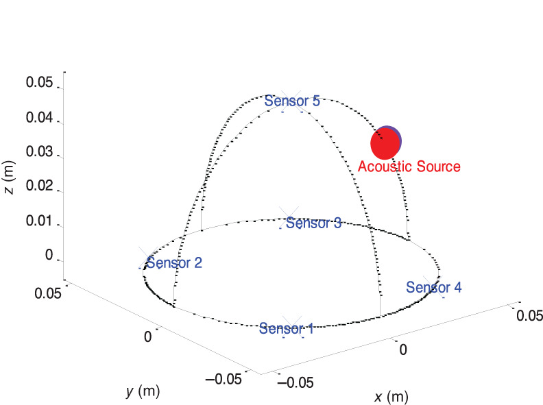
  We have used the magnetoacoustics source description that we developed. They are summarized in Equations ((10), (11), (12)) above. The next step of solving the localization problem was using these calculated TDOAs in the implementation of the hyperbolic positioning equations to get the final location estimation. The localization's results for a specific case are illustrated in Figure 10.

FIGURE 10.

Tumor localization's results for one specific case. The simulated location is marked with a red cross. The algorithm's estimation is given with a purple circle

3.3. In vitro experiment validation

We have prepared a breast phantom with embedded tumor, mimicking the optical properties of breast tissue and a cluster of nanoparticles (nanosonics particles mentioned above, and another that became available later in the market (Ocean Nano Tech.). See Figure 11.

FIGURE 11.

The experimental setup used in the magneto‐acoustic experiment. On the right is a sketch of the system, presenting the sensor array along with the two solenoids and the tissue phantom. On the left is a picture of the actual system containing the tumor phantom within the hemisphere tissue phantom

Since in this setup the solenoids are placed in proximity to the measuring sensors, a very high electromagnetic noise (resulting from the coils) was prone to interfere with the measurement. To evaluate this noise, the tissue phantom was replaced with the control phantom (no tumor). The other system characteristics were maintained the same and a third, 1‐s measurement was taken. As there were no MNPs present in this measurement, no acoustic signal was supposed to appear. Therefore, it contained only the electromagnetic noise and could be used as a reference to eliminate this noise from the “real” measurement. This procedure was repeated for each of the three sensors' combinations in the array. The fourth channel was used for the trigger recording.

The obtained measurements were then transferred to our algorithm for post processing. Each measurement was averaged over the recorded second to get an averaged five‐period segment. To avoid averaging edge effects, the first and last cycles were not used. This averaging reduced the accompanied white noise and eliminated random effects on the signal. To extract the acoustic signal, the averaged electromagnetic noise was then reduced from the obtained averaged signal. Eventually, only the acoustic signal was left and could be implemented for the localization algorithm. Time delays were calculated using threshold crossing with 10 delay vectors that were obtained (10 couples from 5 sensors, seen in Figure 10) and used in the Gauss–Newton algorithm to get the final location estimation. Euclidean distance was calculated to represent the localization error. The measured acoustical signal is shown in Figure 12 (for one sensor only).

FIGURE 12.

The extracted acoustic signal (blue line) gathered by the reduction of the electromagnetic noise from the actual signal. The red line represents the current trigger and highlights the connection between the excitation to the MNP's response. MNP, magnetic nanoparticle

The same analysis was done to all captured signals. Following the acoustic signal extraction, it passed a threshold crossing, yielding a 10‐time delays vector. Using the calculated delays, a final location estimation was achieved with an overlapping volume of 84%. This localization is illustrated in Figure 13

FIGURE 13.

Localization results. The acoustic source and its location estimation are marked by the red and purple circles, respectively

Our paper (Tsalach et al., 2014) was highlighted in the cover of the journal that month (Figure 14) to show its potential for breast cancer imaging as an alternative to current breast imaging methods, with the potential of treatment (that will be discussed next).

FIGURE 14.

Front cover: IEEE Transactions on Biomedical Engineering, Vol. 61, Issue 8, August 2014

4. IN VIVO ANIMALS STUDY

At this stage, we have decided to move to some preliminary mice model experiments. In this study, we combined three modalities. Thermal imaging and magnetoacoustics detection were both discussed at length in this manuscript. The third modality was discussed in the introduction as tumor markers; however, they will play a different role in this study. Fluorescent markers of early apoptosis have the potential to become a powerful tool for cancer treatment monitoring, as they can indicate the number of cells that died during the treatment, and consequently enable the clinician to observe treatment efficacy. Moreover, since these markers can indicate cell death within a short time after treatment, this method can provide the clinician with feedback during the treatment session itself. We have collaborated with Prof. Galia Blum from the Hebrew University in Jerusalem. Prof. Blum co‐authored a Nature Medicine paper that describes treatment response based on AB50‐Cy5 markers for apoptosis (Edgington et al., 2009). We used her markers in the preliminary studies. Eventually, we used the commercial FLIVO 747 markers. We have used our “toolbox” for fluorescent light diffusion in tissue to measure and quantify the signal and its relation to the apoptosis level.

A group of C57BL/J mice were used in this study (11 males in the first group and 8 females); they were each injected with 5 × 10⁵ Lewis lung carcinoma cells. Eleven mice were injected with 100 μl nanoparticles directly in the tumor area. Those mice went through the detection (acoustical, thermal, and fluorescent [after treatment]). The rest of the mice were the control group (tumor injection only). The mice were treated only after tumor volume had exceeded 30 mm³, which happened 8 days on average after injection. Mice were anesthetized by injection of xylazine (20 mg/ml) and ketamine (100 mg/ml). After being anesthetized, each of the mice was positioned between the coils so the tumor was on the line between their centers. The acoustic measurement was performed 0.5 cm away from the tumor. Acoustic measurements were performed before and after nanoparticle injection. After the acoustic measurement, each mouse was taken to the radio frequency (RF) generator for treatment. There were two treatment durations: 6 and 8 min. Field strength was 8 kA/m, while field frequency was 295 kHz. During the treatment, the mouse was thermally isolated from the coil itself and was positioned so that the tumor was in the center of the coil. The thermal camera was placed 45 cm above the mouse to observe thermal changes on the mouse skin. In order to estimate their volume (and therefore to monitor their development), tumors were measured every few days by a caliper. Fluorescence (NIR‐FLIVO® 747 in vivo Apoptosis Tracer) measurements were taken at the following time points: right after the treatment session (−3 h), right before FLIVO injection (0⁻ h), right after FLIVO injection (0⁺ hrs), half an hour after injection (0.5 h), 1 h after injection (1 h), 2 h after injection (2 h) and 3 h after injection (3 h). Each time measurements were taken from the same three points: the treated tumor, the untreated tumor and an area of healthy tissue. Thermal measurements following treatments and fluorescence measurements were in line with expectations. The temperature average of the treated tumor was lower than that of the nontreated. The fluorescence signal exhibit also correlated with the treatment outcome. Further data, images, and analysis can be found in this paper (Shoval et al., 2016). A proposed concept of the diagnostic and treatment is shown in Figure 15.

FIGURE 15.

A basic procedure concept of the multimodal system for detection, treatment and treatment monitoring of cancer

5. MULTIFOCI TUMORS SCENARIO

Until now, we have considered the tumor with one focus only. However, one focus is not always the only case. The presence of a few foci can affect the treatment protocols and the source for the temperature map is a superposition of a few sources that need to be separated to get the correct temperature at the source and to be able to create temperature elevation thermally confined, without damaging healthy tissue. We should bear in mind that we would like to trigger apoptotic cell death. From 42 to 45°C, the apoptotic death mechanism dominates. From 45°C and above, the necrotic death mechanism dominates (Kerr et al., 1994). Therefore, it is essential to have the ability to estimate the temperature at the tumor area.

We went back to the “drawing board” to find a solution to this physical/mathematical problem. We analyzed the problem theoretically, ran simulation, and built a phantom with controllable heat sources at various depths and separation. We will not exhaust the reader with the detailed mathematical analysis and reconstruction algorithm that we developed. We will share with you one figure from Mr. Gil Tamir's thesis (Tamir, 2016) from the lab, and the paper that was published later (Steinberg et al., 2018). See Figure 16.

FIGURE 16.

Surface thermal response to an AC‐stimulated source at different depths. Presented are the different depths and frequency combinations for the DC (constant RF excitation amplitude) and AC (amplitude‐modulated RF excitation amplitude) components. A cross‐section (marked in a dashed white line) through both components is also plotted (a–c: 3 mm and 0.1 Hz; d–f: 5 mm and 0.04 Hz; g–i: 7 mm and 0.033 Hz). RF, radio frequency

The most important takeaway from this analysis is that with a very low modulation frequency of the alternating magnetic, we can separate multiple sources within tissue well.

6. FUTURE WORK

After developing these blocks, the next natural step is to integrate them into one system. The diagram in Figure 17 is the full system as we envision it: SPM nanoparticles specific to tumor surface markers, conjugated with fluorescent tracers of apoptosis; an RF coil creating an AMF for the nanoparticles' excitation. One operating regime for the acoustical signals, and another regime to create heat (the iron‐oxide response). The acoustical signal is collected by an array of acoustical sensors for localization. The surface temperature is collected by a thermal camera. Since the location is determined by the acoustical sensor array, then the temperature at the tumor location can be calculated rather easily. The use of low modulation will also ensure identification of the foci. This will allow the temperature in the tumor location to remain constant between 42 and 45°C for apoptotic death. The feedback will be collected by a fluorescence camera to ensure that this is the case, capturing the fluorophore emission from the interaction site. All of the different components are controlled by one computer/controller.

FIGURE 17.

Fully integrated system with four modalities. RF generator located around the organ of interest for nanoparticle excitation, acoustic sensors array for localization thermal camera for capturing temperature map on the surface, and a fluorescence camera to detect the apoptosis sensing markers. RF, radio frequency

Obviously, the integrated system needs to be tested rigorously on animal models to collect enough data for system refinement and optimization before moving on to human subjects. We have been working with Dr. Elani Liapi, a radiologist who developed a liver cancer model in mice and rabbits (Lee, Liapi, Buijs, Anna Vossen, et al., 2009; Lee, Liapi, Buijs, Vossen, et al., 2009) for the next step in this research. The plan is to work on hepatocellular cancer (HCC), the third most common global cause of cancer‐related death, which usually presents at an advanced stage, allowing patients only palliative treatment options to explore. Among these are image‐guided therapies, such as chemoembolization, which have shown modest patient survival, urging further treatment refinement. Hyperthermia therapy (HT) is an established enhancer of radiation therapy and/or chemotherapy for various types of cancer. Magnetic HT (MHT) involves the injection of MNPs into the tumor with subsequent heating, using AMFs. Exploring MNP's unique ability to generate acoustic waves when in a magnetic field creates a unique opportunity for synchronous imaging and heating. Magnetoacoustic detection offers real‐time MNP visualization, important for treatment planning and thermal monitoring during individualized therapy delivery. We will visualize the gold‐coated MNP after injection into tumors with our magnetoacoustic imaging. By raising RF power, we can heat and measure tissue temperature to control thermal therapy. Modest heating enhances chemotherapeutic effects, with promise for meaningful and cost‐effective patient benefits, including increased survival. We will test whether magnetoacoustic HT‐enhanced chemotherapy will improve unresectable HCC treatment beyond standard‐of‐care chemotherapy. We will first assess local and intratumor MNP distribution with magnetoacoustic detection in a large animal model of liver cancer. We will compare two methods of X‐ray image‐guided injection, and assess MNP distribution with magnetoacoustic imaging, MR R2* mapping, inductively coupled plasma mass spectrometry and quantitative histopathology. We will next characterize local heat distribution in a large animal model of liver cancer. We will measure heat deposition and changes in a large animal model of liver cancer with IR and invasive thermometry. Using prior information on tumor and MNP localization with magnetoacoustics, we will estimate tumor temperature with IR imaging and forecast and compare measured temperature changes in organs and tumors during heating. We will correlate imaging parameters of iron deposition with inductively coupled plasma–mass spectrometry (Masthoff et al., 2019), and imaging parameters of heat with quantitative histopathology and immunohistochemistry, to elucidate associations between tumor and liver iron content and heat distribution, during and after MHT. Subsequently, we will assess treatment efficacy of combined magnetoacoustic MHT and chemotherapy in xenograft mouse models of liver cancer. Success would show that magnetoacoustic MHT has promise for clinical translation for unresectable HCC.

This system is to be used outside the body. It has some limitations in the signal collection from locations deeper than a few centimeters (especially fluorescence), as was pointed out earlier in this manuscript. It can work on human without the fluorescent part, and still, it is a powerful system. It worked well on animals for all signals.

6.1. Minimal invasive system

In Section 1, we referred to our early work on mid‐IR delivery systems, which were flexible fused silica and Teflon waveguides that deliver laser wavelengths in the range of 3–14 μm. We have revisited this research project, and in close collaboration with the late Prof. Jim Harrington, we developed a bundle that transmits energy in this spectral range, specifically optimized to the 8–12 μm (Gal et al., 2010).

See an image of a 900 waveguide coherent bundle in Figure 18:

FIGURE 18.

A coherent bundle composed from 900 individual hollow waveguides, internally coated with silver and silver iodide layers, optimized to deliver energy in the mid‐infrared spectral range to enable thermal image capture

Each of the 900 tubes is internally coated with Ag and AgI, with a thickness that is optimized to the desired 8–12 μm spectral range. We have used this bundle for photothermal measurement of blood oxygen saturation (Milstein et al., 2011). Our interest in transendoscopic application led us to a joint project with Prof. Joseph Rosen on the design of Interferenceless Coded Aperture Correlation Holography Device with Annular Optical Aperture for Endoscopy (Dubey et al., 2020). We plan to implement this special aperture in medical imaging instruments, such as endoscopes and surgical robots, for 3D imaging of internal cavities of the human body, that is, gastrointestinal tracts, the colon, uterus, and stomach. The structure of this device enables insertion of various tools directly onto the main axis of the endoscope channel. The idea is to insert it through the thermal imaging bundle and an RF applicator and acoustic sensor (see Figure 19). All of these devices will extend the operation of our theranostic system within the body cavities. The inner lining of the organ of interest will have the antibody‐coated nanoparticles/apoptotic tracers injected through the blood vessels.

FIGURE 19.

Trans endoscopic theranostic system for procedures within body cavities. 1, endoscope; 2, endoscope distal end; 3, annular optical aperture; 4, thermal imaging bundle (see Figure 18); 5, RF applicator; 6, acoustical sensor (with inflatable balloon to ensure sensor touches the esophagus); 7, nanoparticles on the inner lining of the esophagus

7. SUMMARY AND CONCLUSIONS

We have described in this paper the stages in the development of the individual building blocks that are now integrated into one multimodal theranostic system. The SPM nanoparticles are the basic vehicle that arrives at the tumor area. The gold coating ensures biocompatibility and can be functionalized to conjugate antibodies for specific connectivity to the tumor. Fluorescent markers can be added (by conjugation to the gold surface for apoptosis detection for the system to record). They have the ability to deliver energy and thus elevate the temperature for direct treatment or enhancement of drug performance (which will be concentrated in the tumor area through antibody–antigen reaction using the same vehicle, or be administered to the tumor area separately). Their ability to emit acoustical signals enables precise localization. This information is used to provide an accurate estimate of the temperature at the tumor area, thus allowing efficient treatment with minimal damage to the surrounding tissue. The system is based on four different modalities (RF, thermal, acoustics, and fluorescence), each optimized to perform the image, treat, and monitor. It is worthwhile to mention that the system can utilize additional nanoparticles besides those which we described in this manuscript. Any other nanoparticles that were described in the introduction can be found in the literature if their core has magnetic characteristics. The system is rather small and lightweight and portable. It can easily be transferred on a small cart to be used at the patient's bedside, in the hospital, in outpatient clinics, and even in community clinics or physicians' offices. The final stage of this system as schematically described in Figure 19, extends the use of this method for noninvasive applications.

CONFLICT OF INTEREST

The author has declared no conflicts of interest for this article.

RELATED WIREs ARTICLES

Near‐infrared light‐responsive nanomaterials for cancer theranostics

Gannot, I. (2022). A multimodal nanoparticles‐based theranostic method and system. WIREs Nanomedicine and Nanobiotechnology, 14(4), e1796. 10.1002/wnan.1796

DATA AVAILABILITY STATEMENT

Data available on request from the authors. and some additional data is available on request from the authors

REFERENCES

- Anderson, R. , & Parrish, J. (1981). The optics of human skin. Journal of Investigative Dermatology, 77(1), 13–19. [DOI] [PubMed] [Google Scholar]
- Andrä W, Nowak H. (2007) Magnetism in medicine: A handbook. Wiley‐VCH Verlag GmbH & Co. 10.1002/9783527610174 [DOI] [Google Scholar]
- Becker, W. (2019). The Bh TCSPC handbook (8th ed.). Becker and Hickl. http://www.becker-hickl.de/handbook.htm [Google Scholar]
- Bulte, J. W. M. , & Kraitchman, D. L. (2004). Iron oxide MR contrast agents for molecular and cellular imaging. NMR in Biomedicine, 17, 484–499. 10.1002/nbm.924 [DOI] [PubMed] [Google Scholar]
- Cohen, R., Lide, D., & Trigg, G. (2003). AIP Physics Desk Reference. Springer. [Google Scholar]
- Dana, B. , & Gannot, I. (2012). An analytic analysis of the diffusive‐heat‐flow equation for different magnetic field profiles for a single magnetic nanoparticle. Journal of Physics B: Atomic, Molecular and Optical Physics, 2012, 1–22. 10.1155/2012/135708 [DOI] [Google Scholar]
- Dayan, A. , Goren, A. , & Gannot, I. (2004). Theoretical and experimental investigation of the thermal effects within body cavities during transendoscopical CO2 laser‐based surgery. Lasers in Surgery and Medicine, 35, 18–27. 10.1002/lsm.20061 [DOI] [PubMed] [Google Scholar]
- du, Y. , Jiang, Q. , Beziere, N. , Song, L. , Zhang, Q. , Peng, D. , Chi, C. , Yang, X. , Guo, H. , Diot, G. , Ntziachristos, V. , Ding, B. , & Tian, J. (2016). DNA‐nanostructure–gold‐Nanorod hybrids for enhanced in vivo optoacoustic imaging and photothermal therapy. Advanced Materials, 28(45), 10000–10007. 10.1002/adma.201601710 [DOI] [PubMed] [Google Scholar]
- Dubey, N. , Rosen, J. , & Gannot, I. (2020). High‐resolution imaging system with an annular aperture of coded phase masks for endoscopic applications. Optics Express, 28, 15122–15137. 10.1364/oe.391713 [DOI] [PubMed] [Google Scholar]
- Duck FA. (1990). Physical properties of tissue. A comprehensive reference book. Academic Press. [Google Scholar]
- Edgington, L. E. , Berger, A. B. , Blum, G. , Albrow, V. E. , Paulick, M. G. , Lineberry, N. , & Bogyo, M. (2009). Noninvasive optical imaging of apoptosis by caspase‐targeted activity‐based probes. Nature Medicine, 15(8), 967–973. 10.1038/nm.1938 [DOI] [PMC free article] [PubMed] [Google Scholar]
- Eruv, T. , Ben‐David, M. , & Gannot, I. (2008). An alternative approach to analyze fluorescence lifetime images as a base for a tumor early diagnosis system. IEEE Journal of Selected Topics in Quantum Electronics, 14(1), 98–104. 10.1109/JSTQE.2007.913978 [DOI] [Google Scholar]
- Filippi, L. , Chiaravalloti, A. , Schillaci, O. , Cianni, R. , & Bagni, O. (2020). Theranostic approaches in nuclear medicine: Current status and future prospects. Expert Review of Medical Devices, 17(4), 331–343. 10.1080/17434440.2020.1741348 [DOI] [PubMed] [Google Scholar]
- Gal, U. , Harrington, J. , Ben‐David, M. , Bledt, C. , Syzonenko, N. , & Gannot, I. (2010). Coherent hollow‐core waveguide bundles for thermal imaging. Applied Optics, 49(25), 4700–4709. 10.1364/AO.49.004700 [DOI] [PubMed] [Google Scholar]
- Gandjbakhche, A. H. , & Weiss, G. H. (1995). V: Random walk and diffusion‐like models of photon migration in turbid media. Progress in Optics, 34, 333–402. 10.1016/S0079-6638(08)70328-7 [DOI] [Google Scholar]
- Gannot, I. , Dror, J. , Calderon, S. , Kaplan, I. , & Croitoru, N. (1994). Flexible waveguides for IR laser radiation and surgery applications. Lasers in Surgery and Medicine, 14(2), 189. 10.1002/1096-9101(1994)14:2<184::AID-LSM1900140212>3.0.CO;2-U [DOI] [PubMed] [Google Scholar]
- Gannot, I. , Ron, I. , Hekmat, F. , Chernomordik, V. , & Gandjbakhche, A. (2004). Functional optical detection based on pH dependent fluorescence lifetime. Lasers in Surgery and Medicine, 35(5), 342–348. 10.1002/lsm.20101 [DOI] [PubMed] [Google Scholar]
- Goren, A. , Dayan, A. , & Gannot, I. (2003). Transendoscopic laser based surgical procedure within body cavities. In Proceedings of the Optical Fibers and Sensors for Medical Applications III; (Vol. 4957). SPIE—The International Society for Optical Engineering. 10.1117/12.478068 [DOI] [Google Scholar]
- Gustafsson, F. , & Gunnarsson, F. (2003). Positioning using time‐difference of arrival measurements. In ICASSP, IEEE International Conference on Acoustics, Speech and Signal Processing—Proceedings. 10.1109/icassp.2003.1201741 [DOI] [Google Scholar]
- Herrmann, K. , Larson, S. M. , & Weber, W. A. (2017). Theranostic concepts: More than just a fashion trend‐introduction and overview. Journal of Nuclear Medicine, 58, 1S–2S. 10.2967/jnumed.117.199570 [DOI] [PubMed] [Google Scholar]
- Hofmann‐Wellenhof B, Legat K, Wieser M. (2003). Navigation‐Principles of Positioning and Guidance. Springer. [Google Scholar]
- Hu, G. , Tang, J. , Bai, X. , Xu, S. , & Wang, L. (2016). Superfluorinated copper sulfide nanoprobes for simultaneous 19F magnetic resonance imaging and photothermal ablation. Nano Research, 9(6), 1630–1638. 10.1007/s12274-016-1057-2 [DOI] [Google Scholar]
- Jacques, S. L. (2013). Erratum: Optical properties of biological tissues: A review. Physics in Medicine and Biology, 58(14), R37–R61. 10.1088/0031-9155/58/14/5007 [DOI] [PubMed] [Google Scholar]
- Jones, S. , & Thornton, J. M. (1996). Principles of protein‐protein interactions. Proceedings of the National Academy of Sciences of the United States of America, 93, 13–20. 10.1073/pnas.93.1.13 [DOI] [PMC free article] [PubMed] [Google Scholar]
- Kalambur, V. S. , Han, B. , Hammer, B. E. , Shield, T. W. , & Bischof, J. C. (2005). In vitro characterization of movement, heating and visualization of magnetic nanoparticles for biomedical applications. Nanotechnology, 16, 1221–1233. 10.1088/0957-4484/16/8/041 [DOI] [Google Scholar]
- Kelkar, S. S. , & Reineke, T. M. (2011). Theranostics: Combining imaging and therapy. Bioconjugate Chemistry, 22(10), 1879–1903. 10.1021/bc200151q [DOI] [PubMed] [Google Scholar]
- Kerr, J. F. R. , Winterford, C. M. , & Harmon, B. V. (1994). Apoptosis. Its significance in cancer and cancer therapy. Cancer, 73(8), 2013–2026. 10.1002/1097-0142(19940415)73:8<2013::AID-CNCR2820730802>3.0.CO;2-J [DOI] [PubMed] [Google Scholar]
- Lee, K. H. , Liapi, E. , Buijs, M. , Anna Vossen, J. , Prieto‐Ventura, V. , Syed, L. H. , & Geschwind, J. F. H. (2009). Percutaneous US‐guided implantation of Vx‐2 carcinoma into rabbit liver: A comparison with open surgical method. The Journal of Surgical Research, 155(1), 94–99. 10.1016/j.jss.2008.08.036 [DOI] [PMC free article] [PubMed] [Google Scholar]
- Lee, K. H. , Liapi, E. , Buijs, M. , Vossen, J. , Hong, K. , Georgiades, C. , & Geschwind, J. F. H. (2009). Considerations for implantation site of VX2 carcinoma into rabbit liver. Journal of Vascular and Interventional Radiology, 20, 113–117. 10.1016/j.jvir.2008.09.033 [DOI] [PMC free article] [PubMed] [Google Scholar]
- Levy, A. , Dayan, A. , Ben‐David, M. , & Gannot, I. (2010). A new thermography‐based approach to early detection of cancer utilizing magnetic nanoparticles theory simulation and in vitro validation. Nanomedicine: Nanotechnology, Biology, and Medicine, 6(6), 786–796. 10.1016/j.nano.2010.06.007 [DOI] [PubMed] [Google Scholar]
- Masthoff, M. , Buchholz, R. , Beuker, A. , Wachsmuth, L. , Kraupner, A. , Albers, F. , Freppon, F. , Helfen, A. , Gerwing, M. , Höltke, C. , Hansen, U. , Rehkämper, J. , Vielhaber, T. , Heindel, W. , Eisenblätter, M. , Karst, U. , Wildgruber, M. , & Faber, C. (2019). Introducing specificity to iron oxide nanoparticle imaging by combining 57Fe‐based MRI and mass spectrometry. Nano Letters, 19(11), 7908–7917. 10.1021/acs.nanolett.9b03016 [DOI] [PubMed] [Google Scholar]
- Milstein, Y. , Tepper, M. , David, M. B. , Harrington, J. A. , & Gannot, I. (2011). Photothermal bundle measurement of phantoms and blood as a proof of concept for oxygenation saturation measurement. Journal of Biophotonics, 4(4), 219–223. 10.1002/jbio.201000055 [DOI] [PubMed] [Google Scholar]
- Overgaard, J. , Gonzalez Gonzalez, D. , Hulshof, M. C. C. H. , Arcangeli, G. , Dahl, O. , Mella, O. , & Bentzen, S. M. (2009). Hyperthermia as an adjuvant to radiation therapy of recurrent or metastatic malignant melanoma. A multicentre randomized trial by the European Society for Hyperthermic Oncology. International Journal of Hyperthermia, 25, 323–334. 10.1080/02656730903091986 [DOI] [PubMed] [Google Scholar]
- Peng, Y. , Liu, Y. , Lu, X. , Wang, S. , Chen, M. , Huang, W. , Wu, Z. , Lu, G. , & Nie, L. (2018). Ag‐hybridized plasmonic Au‐triangular nanoplates: Highly sensitive photoacoustic/Raman evaluation and improved antibacterial/photothermal combination therapy. Journal of Materials Chemistry B, 6(18), 2813–2820. 10.1039/c8tb00617b [DOI] [PubMed] [Google Scholar]
- Pennes, H. H. (1948). Analysis of tissue and arterial blood temperatures in the resting human forearm. Journal of Applied Physiology, 1, 93–122. 10.1152/jappl.1948.1.2.93 [DOI] [PubMed] [Google Scholar]
- Rosensweig, R. E. (2002). Heating magnetic fluid with alternating magnetic field. Journal of Magnetism and Magnetic Materials, 252, 370–374. 10.1016/S0304-8853(02)00706-0 [DOI] [Google Scholar]
- Seidlin, S. M. , Marinelli, L. D. , & Oshry, E. (1946). Radioactive iodine therapy‐effect on functioning metastases of adenocarcinoma of the thyroid. Journal of the American Medical Association, 132(14), 838–847. [DOI] [PubMed] [Google Scholar]
- Sheriff, S. (1990). Antibody‐antigens complexes. Annual Review of the Biochemistry, 59, 439–473. [DOI] [PubMed] [Google Scholar]
- Shoval, A. , Tepper, M. , Tikochkiy, J. , Gur, L. B. , Markovich, G. , Keisari, Y. , & Gannot, I. (2016). Magnetic nanoparticles‐based acoustical detection and hyperthermic treatment of cancer, in vitro and in vivo studies. Journal of Nanophotonics, 10(3), 036007. 10.1117/1.JNP.10.036007 [DOI] [Google Scholar]
- Solnes, L. B. , Werner, R. A. , Jones, K. M. , Sadaghiani, M. S. , Bailey, C. R. , Lapa, C. , Pomper, M. G. , & Rowe, S. P. (2020). Theranostics: Leveraging molecular imaging and therapy to impact patient management and secure the future of nuclear medicine. Journal of Nuclear Medicine, 61(3), 311–318. 10.2967/jnumed.118.220665 [DOI] [PubMed] [Google Scholar]
- Steinberg, I. , Ben‐David, M. , & Gannot, I. (2012). A new method for tumor detection using induced acoustic waves from tagged magnetic nanoparticles. Nanomedicine: Nanotechnology, Biology, and Medicine, 8(5), 569–579. 10.1016/j.nano.2011.09.011 [DOI] [PubMed] [Google Scholar]
- Steinberg, I. , Tamir, G. , & Gannot, I. (2018). A reconstruction method for the estimation of temperatures of multiple sources applied for nanoparticle‐mediated hyperthermia. Molecules, 23(3), 670–686. 10.3390/molecules23030670 [DOI] [PMC free article] [PubMed] [Google Scholar]
- Tabish, T. A. , Dey, P. , Mosca, S. , Salimi, M. , Palombo, F. , Matousek, P. , & Stone, N. (2020). Smart gold nanostructures for light mediated cancer theranostics: Combining optical diagnostics with photothermal therapy. Advancement of Science, 7(15), 1–28. 10.1002/advs.201903441 [DOI] [PMC free article] [PubMed] [Google Scholar]
- Tamir G. (2016). 3D temperature mapping for monitoring of tumor’s localized hyperthermia treatment. Master Thesis, Tel‐Aviv University.
- Tsalach A. (2012). Time difference of arrival based cancer tumor localization using magnetic nanoparticles induced acoustic signals. Master Thesis, Tel‐Aviv University.
- Tsalach, A. , Steinberg, I. , & Gannot, I. (2014). Tumor localization using magnetic nanoparticle‐induced acoustic signals. IEEE Transactions on Biomedical Engineering, 61(8), 2313–2323. 10.1109/TBME.2013.2286638 [DOI] [PubMed] [Google Scholar]
- Wang, L. , Jacques, S. L. , & Zheng, L. (1995). MCML‐Monte Carlo modeling of light transport in multi‐layered tissues. Computer Methods and Programs in Biomedicine, 47, 131–146. 10.1016/0169-2607(95)01640-F [DOI] [PubMed] [Google Scholar]
- Yifat, J. , & Gannot, I. (2015). 3D discrete angiogenesis dynamic model and stochastic simulation for the assessment of blood perfusion coefficient and impact on heat transfer between nanoparticles and malignant tumors. Microvascular Research, 98, 197–217. 10.1016/j.mvr.2014.01.006 [DOI] [PubMed] [Google Scholar]
- Zhao, Y. , Liu, W. , Tian, Y. , Yang, Z. , Wang, X. , Zhang, Y. , Tang, Y. , Zhao, S. , Wang, C. , Liu, Y. , Sun, J. , Teng, Z. , Wang, S. , & Lu, G. (2018). Anti‐EGFR peptide‐conjugated triangular gold nanoplates for computed tomography/photoacoustic imaging‐guided photothermal therapy of non‐small cell lung cancer. ACS Applied Materials & Interfaces, 10(20), 16992–17003. 10.1021/acsami.7b19013 [DOI] [PubMed] [Google Scholar]
Associated Data
This section collects any data citations, data availability statements, or supplementary materials included in this article.