Abstract
Background
Training deep learning (DL) models to automatically recognize diseases in nasopharyngeal MRI is a challenging task, and optimizing the performance of DL models is difficult.
Purpose
To develop a method of training anatomical partition‐based DL model which integrates knowledge of clinical anatomical regions in otorhinolaryngology to automatically recognize diseases in nasopharyngeal MRI.
Study Type
Single‐center retrospective study.
Population
A total of 2485 patients with nasopharyngeal diseases (age range 14–82 years, female, 779[31.3%]) and 600 people with normal nasopharynx (age range 18–78 years, female, 281[46.8%]) were included.
Sequence
3.0 T; T2WI fast spin‐echo sequence.
Assessment
Full images (512 × 512) of 3085 patients constituted 100% of the dataset, 50% and 25% of which were randomly retained as two new datasets. Two new series of images (seg112 image [112 × 112] and seg224 image [224 × 224]) were automatically generated by a segmentation model. Four pretrained neural networks for nasopharyngeal diseases classification were trained under the nine datasets (full image, seg112 image, and seg224 image, each with 100% dataset, 50% dataset, and 25% dataset).
Statistical Tests
The receiver operating characteristic curve was used to evaluate the performance of the models. Analysis of variance was used to compare the performance of the models built with different datasets. Statistical significance was set at P < 0.05.
Results
When the 100% dataset was used for training, the performances of the models trained with the seg112 images (average area under the curve [aAUC] 0.949 ± 0.052), seg224 images (aAUC 0.948 ± 0.053), and full images (aAUC 0.935 ± 0.053) were similar (P = 0.611). When the 25% dataset was used for training, the mean aAUC of the models that were trained with seg112 images (0.823 ± 0.116) and seg224 images (0.765 ± 0.155) was significantly higher than the models that were trained with full images (0.640 ± 0.154).
Data Conclusion
The proposed method can potentially improve the performance of the DL model for automatic recognition of diseases in nasopharyngeal MRI.
Level of Evidence
4
Technical Efficacy Stage
1
Keywords: deep learning, automatic segmentation, nasopharyngeal region, MRI recognition, anatomical partition
Training artificial intelligence (AI) models to automatically recognize diseases in medical images has been a topic of interest in recent years. 1 , 2 Automatic recognition of diseases in nasopharyngeal MRI is one of the most challenging tasks in this field and several studies have made efforts. For example, Wong et al conducted a study to automatically detect early‐stage nasopharyngeal carcinoma (NPC) and discriminate it from benign hyperplasia using noncontrast‐enhanced MRI. 3 Ke et al developed a dual‐task deep learning (DL) model to detect and segment NPC automatically in MRI. 4 However, these studies focused on NPC, and the methods employed do not delve on the specificity of medical imaging itself.
MRI has special features that differ from nonmedical imaging. The naming and classification of diseases are closely related to anatomy. For example, otorhinolaryngology MRI can be clinically divided into the following areas: nasal cavity, paranasal sinus, orbit, middle skull base, nasopharynx, parapharyngeal spaces, temporal area, lateral skull base, and intracranial areas. Rather than being randomly located in the image like a cat in a picture, most diseases are in a corresponding anatomical area in the image. For example, adenoids would always be in the nasopharynx and never in the temporal area. Therefore, we believe that it would be better to train a DL model to recognize diseases of nasopharyngeal MRI based on anatomical partitions than based on the full image.
The aim of this study was to evaluate whether a method of training DL models using MRI based on anatomical partition, which integrates knowledge of clinical anatomical region division in otorhinolaryngology, improved model performance for nasopharyngeal diseases classification and reduced data costs compared to the traditional methods based on full images.
Materials and Methods
Patients Information
The study protocol was approved by the Institutional Review Board of the authors' institution, and the requirement to obtain informed consent from the patients was waived. Since this study was defined as a methodological study, only images of nasopharyngeal diseases rather than all diseases of nasopharynx were collected to determine the advantages of the proposed methodology. A total of 3085 nasopharyngeal MRI scans, including those with NPC, nasopharyngeal lymphoid hyperplasia (LH), nasopharyngeal lymphoma, chordoma invading the nasopharynx, craniopharyngioma invading the nasopharynx, and normal nasopharynx (from 600 participants with normal nasopharynx and tumor‐free slices of the above lesions) produced between January 1, 2014 and December 31, 2020, were retrospectively collected (Table 1). Patient information are described in detail in the Patients and Image Acquisition section of the Supporting Information.
TABLE 1.
Characteristics of Patients in the Training and Test Cohorts
| Training Cohort Slices (Patient) | Test Cohort Slices (Patient) | Total Slices (Patient) | Age Range (year) | Sex | ||
|---|---|---|---|---|---|---|
| M | F | |||||
| NPC | 4529 (1369) | 992 (454) | 5521(1823) | 16–82 | 1302 | 521 |
| LH | 231 (159) | 71 (53) | 302 (212) | 14–67 | 97 | 115 |
| Lymphoma | 152 (85) | 38 (29) | 190 (114) | 14–81 | 83 | 31 |
| Chordoma | 362 (84) | 115 (29) | 377 (113) | 14–76 | 78 | 35 |
| Craniopharyngioma | 328 (169) | 75 (54) | 403 (223) | 14–77 | 146 | 77 |
| Normal | 4375 (‐) | 1353 (‐) | 5728 (‐) | ‐ | ‐ | ‐ |
| Total | 9977 (1866) | 2644 (619) | 12621 (2485) | 14–82 | 1706 | 779 |
The training and test groups were divided by patient as a unit, according to an approximate ratio of 3:1. For all categories of diseases, we only selected the slices with a visible mass near the nasopharyngeal area, and the slices with a mass that was very small or beyond the perinasopharyngeal area were not included. The images of the normal nasopharynx were obtained from the MRIs of 600 people undergoing routine physical examinations and nontumor slices in the perinasopharyngeal area of the MRIs of the five diseases mentioned. As the number of these patients cannot be effectively determined, “‐” is used.
NPC = nasopharyngeal carcinoma; LH = nasopharyngeal lymphatic hyperplasia; Normal = normal nasopharynx; M = Male; F = Female.
MRI Data Acquisition
MRI was obtained using 3.0‐T MR imaging systems (GE, Discovery MR 750 and Signa HDxt). Axial T2‐weighted images collected in DICOM format were acquired. The parameters for the images were as follows: repetition time 2699–4480 msec, echo time 67–117 msec, flip angle 111°–142°, slice thickness 4–6 mm, pixel size 1.25 mm × 1.25 mm, and matrix size 512 × 512.
Image Processing
To build models that could automatically segment the perinasopharyngeal area and recognize diseases in this area, datasets for training segmentation DL models and for training nasopharyngeal disorders classification DL models need to be prepared.
Dataset for Training Segmentation DL Models
Six hundred slices were randomly selected from all categories of disease images to establish the dataset. The perinasopharyngeal area in the image was marked using the ITK‐SNAP software (Version 3.6.0, University of Pennsylvania, Philadelphia, PA, USA). 5 The task was performed by a junior otolaryngologist (L.S., with 3 years of experience) and reviewed by another senior otolaryngologist (D.Y.Q., with 10 years of experience). The definition of the perinasopharyngeal area was described in the Dataset for Segmentation section of Supporting Information.
Dataset for Training Classification DL Models
The dataset of the classification model included a total of 12,621 images. The patients in each category were divided into a training cohort and a test cohort in a 3:1 ratio. To explore whether the method of training DL models based on anatomical partition has the advantage of reducing data costs, we randomly assigned 50% images and 25% images of the training cohort of each category to form two new datasets (50% and 25% dataset) and compared the performances of the DL models trained in different datasets. Furthermore, to explore whether the method of training DL models based on anatomical partition can improve the performance of the DL model compared to the traditional method based on the full image (512 × 512), the better‐performing segmentation DL model was employed to construct two new image formats (the seg112 image [112 × 112] and seg224 image [224 × 224]) from the full images. To obtain a seg112 image, the geometric center of the segmentation region predicted by the employed segmentation DL model was extended 56 pixels up, down, left, and right, respectively, to form a 112 × 112 square segmentation region. The seg224 image was obtained by extending the geometric center by 112 pixels using the same method. Therefore, nine datasets (full image, seg112 image, and seg224 image, each with 100% dataset, 50% dataset, and 25% dataset) were created for training the nasopharyngeal diseases classification DL models.
Network Architecture
Our platform was based on the Pytorch library (version 1.9.0) with CUDA (version 10.0) for GPU (NVIDIA Tesla T4, NVIDIA corporation, Santa Clara, CA, USA) acceleration on a Windows operating system (Server 2019 data center version 64 bit, 8 vCPU 31 GiB). The U‐net 6 and the Deeplabv3 7 were used to build the semantic segmentation models (Fig. 1). The U‐net and the Deeplabv3 were used to build the semantic segmentation models while the RMSprop optimizer was used to train the models with a batch size of 32, and the initial learning rate was set to 0.001. Both semantic segmentation models were trained for 40 epochs. Four common pretrained DL networks were transferred for diseases classification DL models building: EfficientNet‐B0, 8 Legacy SE‐ResNet34, 9 MobileNetV3 Large100, 10 and DenseNet121. 11 The nine datasets were used for training each model separately. Therefore, a total of 36 (4 × 9) DL models for nasopharyngeal diseases classification were established (Fig. 2). The stochastic gradient descent (SGD) optimizer was used to train the networks with a batch size of 32, the initial learning rate was set to 0.001, and each model was trained for 40 epochs.
FIGURE 1.
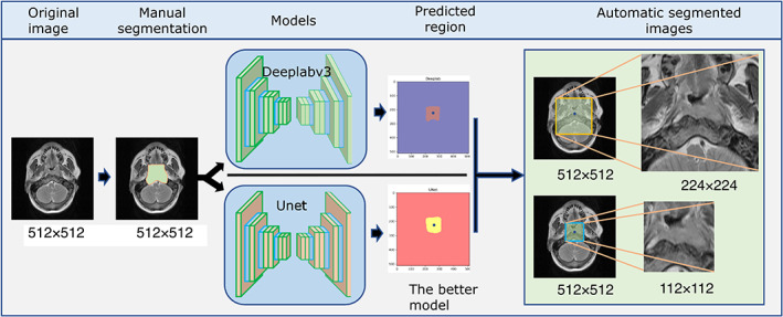
Semantic segmentation models based on U‐net and Deeplabv3 were trained to automatically generate the seg112 and seg224 images.
FIGURE 2.
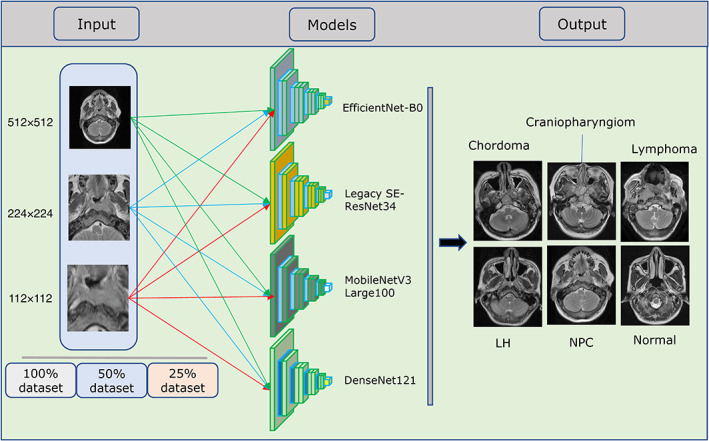
Training of the four neural networks using the nine datasets (full, seg112, and seg224 images, each with 100%, 50%, and 25% datasets). LH = nasopharyngeal lymphoid hyperplasia; NPC = nasopharyngeal carcinoma.
Quantitative Evaluation Scheme of Interpretability
The interpretability of the models is extremely important when AI is applied in the medical field. When the prediction basis of an AI model is not well understood and if it is unknown when it may be wrong, it is difficult to entrust medical decisions from its results, especially since neural networks are often described as black box models. 12 , 13 Considering that interpretability differs significantly between tasks because it is highly subjective and the Grad‐CAM, 14 which is generated based on neural network feature engineering, does not allow for a quantitative evaluation of the model's interpretability, we developed a quantitative evaluation scheme for Grad‐CAM in a group that included two radiologists after consulting with an AI expert (G.X.Q. from School of Computer Science, Wuhan University). The quantitative evaluation of the interpretability of the DL model was developed based on the experience of the radiologists in diagnosing nasopharyngeal lesions (mainly based on the internal features of the mass). The evaluation criteria were set as follows: almost all the bright yellow areas on Grad‐CAM were on the mass, 1 point; most of the bright yellow areas were on the mass, 0.75 points; approximately half of the bright yellow areas were on the mass, 0.5 points; only few yellow bright areas were on the mass, 0.25 points; and almost all bright yellow areas were not on the mass, 0 points (Fig. 3). Two otolaryngologists (L.S. with 5 years of experience and Z.Z.L. with 4 years of experience) and a radiologist (C.X.X. with 15 years of experience) independently scored each correctly classified Grad‐CAM images and calculated the average Grad‐CAM score of each model.
FIGURE 3.
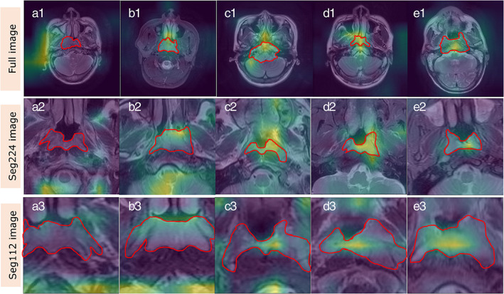
Evaluation rules of interpretability of deep learning (DL) model. The red area represents the area where the lesion is located, and the yellow‐green bright area is the extracted feature maps which indicates the classification basis of the model. The Grad‐CAM diagrams of A1, A2, and A3 show that the features extracted by the model are almost not in the lesion area, which is rated as 0; B1, B2, and B3 show that only a small part of the features extracted by the model are in the lesion area, which is rated as 0.25 points; C1, C2, and C3 show that about half of the features extracted by the model are in the lesion area, which is rated as 0.5 points; D1, D2, and D3 show that most of the features extracted by the model are in the lesion area, which is rated as 0.75; E1, E2, and E3 show that almost all the features extracted by the model are in the lesion area, which is rated as 1 point.
Statistical Analysis
Dice similarity coefficients (Dice) were used to evaluate the performance of the semantic segmentation models. The receiver operating characteristic (ROC) curves were used to evaluate the performance of classification models. As there were 36 classification models in this study, the mean value of the area under the curve (AUC) of each model for each dataset was calculated to facilitate the analysis of the results. The AUC of each model for each disease was grouped based on the 100%, 50%, and 25% datasets, respectively, and analysis of variance was used to compare the performance of the models built with the three datasets. Independent samples t‐test was used to compare Grad‐CAM score. Analyses were performed using IBM SPSS Statistics for Windows, version 24.0 (IBM Corp., Armonk, NY, USA). Statistical significance was set at P < 0.05.
Results
Results of the Semantic Segmentation Models
After 40 epochs of training, the performances of U‐net and Deeplabv3 quickly stabilized. The Dice scores of the U‐net and Deeplabv3 were 0.805 ± 0.021 and 0.897 ± 0.029, respectively. Because the performance of Deeplabv3 was better than that of U‐net, the seg112 and seg224 images were generated from the full images using the trained Deeplabv3. The examples of segmentation for both models are displayed in Fig. 4.
FIGURE 4.
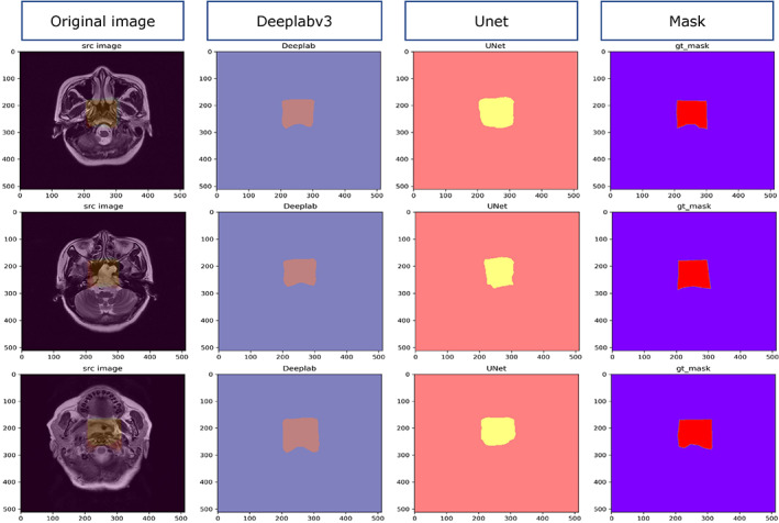
Segmentation examples of U‐net and Deeplabv3.
Performance of Classification Models
When the 100% dataset was used as the training dataset of the models, the aAUCs of the EfficientNet‐B0, Legacy SE‐ResNet34, MobileNetV3 Large100, and DenseNet121 trained with seg112 images were 0.955 ± 0.064, 0.943 ± 0.051, 0.957 ± 0.043, and 0.942 ± 0.059, respectively, while for those trained with seg224 images, the aAUCs were 0.965 ± 0.036, 0.937 ± 0.077, 0.943 ± 0.050, and 0.947 ± 0.054, respectively, and for those trained with full images, the aAUCs were 0.940 ± 0.055, 0.928 ± 0.061, 0.935 ± 0.047, and 0.938 ± 0.063, respectively (Fig. 5). When evaluated using the ROC curve, the DL models trained with the 100% dataset show similar performance with the seg112, seg224, and full images (P = 0.611). The mean aAUC of the four DL models trained with the full image (0.935 ± 0.053) was 0.014 and 0.013 lower than the mean aAUC of the four DL models trained with the seg112 image (0.949 ± 0.052) and seg224 image (0.948 ± 0.053), respectively (Fig. 6).
FIGURE 5.
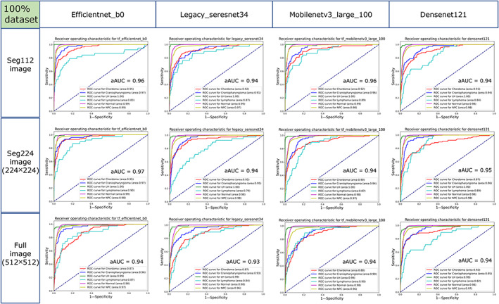
Receiver operating characteristic (ROC) curves of the EfficientNet‐B0, Legacy SE‐ResNet34, MobileNetV3 Large100, and DenseNet121 trained with the seg112, seg224, and full images using the 100% dataset in the test cohort. aAUC = average area under the curve of the six categories.
FIGURE 6.
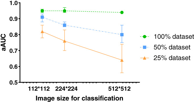
Average areas under the curve (aAUCs) of the models trained with different image sizes (112 × 112, 224 × 224, and 512 × 512) using 100%, 50%, and 25% datasets in the test cohort.
When the 50% dataset was used as the training dataset of the models, the aAUCs of the EfficientNet‐B0, Legacy SE‐ResNet34, MobileNetV3 Large100, and DenseNet121 networks trained with seg112 images were 0.905 ± 0.085, 0.925 ± 0.054, 0.875 ± 0.112, and 0.915 ± 0.064, respectively, while for those trained with seg224 images, the aAUCs were 0.875 ± 0.099, 0.862 ± 0.095, 0.863 ± 0.111, and 0.845 ± 0.084, respectively, and for those trained with full images, the aAUCs were 0.863 ± 0.132, 0.833 ± 0.089, 0.772 ± 0.155, and 0.753 ± 0.145, respectively (Fig. 7). The performances of the DL models trained with the 50% dataset were significantly lower than those of the neural networks trained with the 100% dataset (Fig. 6). Among them, the performance with the seg112 images dropped by 0.044, seg224 images by 0.087, and full images by 0.130. The MobileNetV3 Large100 and DenseNet121 trained with the full images lost the ability to discriminate chordoma (AUC is close to 0.5).
FIGURE 7.
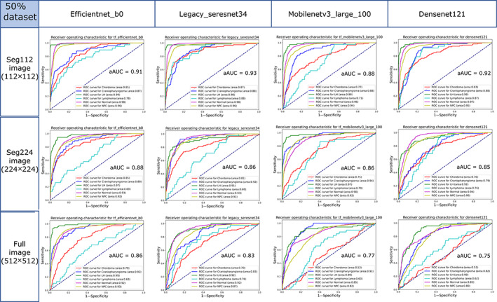
Receiver operating characteristic (ROC) curves of the EfficientNet‐B0, Legacy SE‐ResNet34, MobileNetV3 Large100, and DenseNet121 trained with the seg112, seg224, and full images using the 50% dataset in the test cohort. aAUC = average area under the curve of the six categories.
When the 25% dataset was used as the training dataset of the models, the aAUCs of the EfficientNet‐B0, Legacy SE‐ResNet34, MobileNetV3 Large100, and DenseNet121 networks trained with the seg112 images were 0.863 ± 0.116, 0.830 ± 0.107, 0.777 ± 0.136, and 0.820 ± 0.118, respectively, while for those trained with seg224 images, the aAUCs were 0.830 ± 0.094, 0.797 ± 0.155, 0.697 ± 0.199, and 0.735 ± 0.156, respectively, and for those trained with full images, the aAUCs were 0.740 ± 0.139, 0.662 ± 0.126, 0.560 ± 0.186, and 0.597 ± 0.117, respectively (Fig. 8). The mean aAUC of the four DL models trained with the full image (0.640 ± 0.154) was significantly lower than the mean aAUC of the four DL models trained with the seg112 image (0.823 ± 0.116) and the seg224 image (0.765 ± 0.155), respectively (Fig. 6). The performances of the four neural networks trained with the 25% dataset were significantly lower than those of the neural network trained with the 50% dataset. The ROC curves of MobileNetV3 Large100 and DenseNet121 trained with the full images almost collapsed, and they lost the ability to discriminate most diseases (the AUC of the model is close to 0.5 for most diseases), and the best‐performing EfficientNet‐B0 lost the ability to discriminate chordoma (AUC = 0.53). Furthermore, the classification ability of the models trained with the seg224 images began to decline sharply.
FIGURE 8.
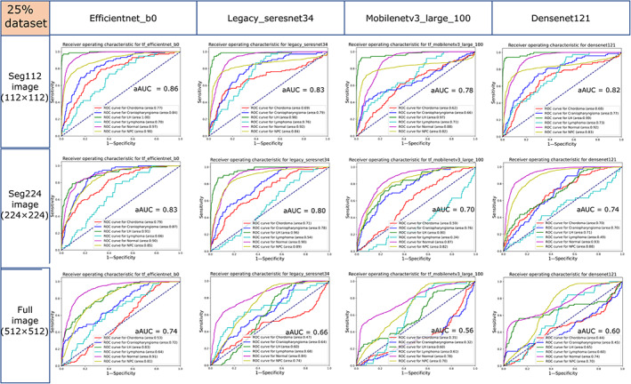
Receiver operating characteristic (ROC) curves of the EfficientNet‐B0, Legacy SE‐ResNet34, MobileNetV3 Large100, and DenseNet121 trained with the seg112, seg224, and full images using the 25% dataset in the test cohort. aAUC = average area under the curve of the six categories.
Evaluation of Interpretability
In the test cohort of each disease category under the 100% dataset of the full, seg224, and seg112 images, the four trained neural networks generated a total of 31,728 Grad‐CAM images. Figure 9 presents the evaluation results of each model by reviewers 1, 2, and 3. The results show that the interpretability of the model trained by the seg112 images (0.735 ± 0.097) is significantly better than those of the models trained by the seg224 (0.242 ± 0.037) and full images (0.245 ± 0.043). Examples of the Grad‐CAM images of the four trained neural networks for the five types of diseases and normal nasopharynx are presented in the Results section of the Supporting Information.
FIGURE 9.
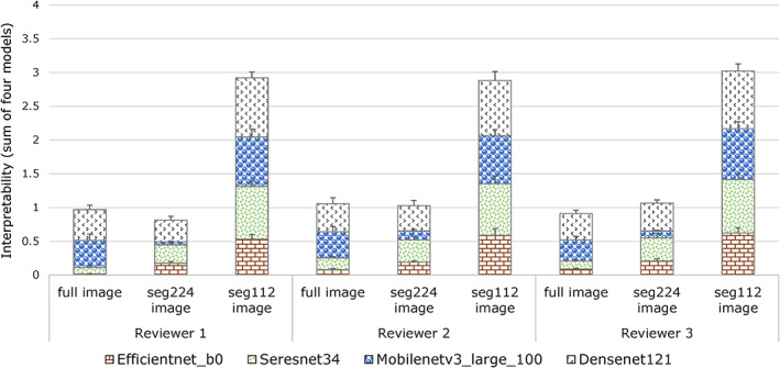
Interpretability of the four models evaluated by reviewer 1, reviewer 2, and reviewer 3.
Discussion
In this study, using the nasopharyngeal region on MRI as an example, we developed a method of training anatomical partition‐based DL model for automatic disease recognition using nasopharyngeal MRI. The results indicate that the method enabled the DL model to perform better with a small dataset compared with the traditional method. Moreover, we established a quantitative evaluation method for evaluating interpretability of the DL model based on the characteristics of the tasks in this study. The results indicate that the training method we developed equips the DL model with better interpretability.
Traditional machine learning models for classification tasks, such as the classic cat and dog recognition model, 15 label the images and input them into the network for training, which could not reflect prior knowledge. The same strategy is used in many medical image processing tasks. 16 , 17 However, medical images possess special features that differ from nonmedical images. For example, the pixels that represent animals can be anywhere in the image, whereas anatomically based diseases tend to be in a corresponding anatomical area in MRI. To reflect this difference and provide the model with prior anatomical knowledge, we envisioned that when training DL models to automatically recognize diseases on MRI, the whole image can be anatomically decomposed. The results are in line with our assumptions that the performance of the models trained with the seg112 image is better than those trained with the full image under the same training dataset and the performance of the models trained with the full image decreases sharply when the size of the training dataset is reduced. Whereas, the models trained with the seg112 image maintained adequate performance even with the 25% dataset. Medical image analysis method using neural networks based on limited data is an important issue to be addressed. Since the incidence of different diseases varies considerably, only small datasets exist for many diseases, and data imbalance is common in medicine. The issue of training a robust DL model with a small dataset needs to be addressed urgently. Computer experts are committed to constructing effective mathematical algorithms to enable AI to extract valuable information from limited images. 18 , 19 However, the special features that make medical images different from nonmedical pictures have not been paid enough attention. Our training method provides a feasible solution from a physician's perspective.
Since the interpretability of the DL model is closely related to medical safety, it is difficult to entrust medical decisions based on results from AI in which the prediction basis is not yet well understood, especially since the neural network is usually described as a black box. 12 , 13 Many studies have claimed that a DL model has achieved a high level of performance for a specific task, but the interpretability of the model has not been evaluated. 20 , 21 The prediction of the networks may be based on information that is unrelated to prior medical knowledge. Our results showed that the models trained with the seg112 images had better interpretability compared with the models trained with the full images, which further affirms the potential of the developed method in this study.
Another potential advantage of the developed method in realizing automatic MRI recognition in the future is that the training and update costs of the DL model will be reduced. Training a DL model for automatic recognition of diseases in MRI based on traditional methods requires sufficient disease data to be collected at one time. For example, MRI at the nasopharyngeal level includes the temporal bone region, nasal cavity and paranasal sinus region, orbital region, intracranial region, nasopharyngeal region, and parapharyngeal space region. There are a variety of diseases in each region, and the availability of image data from many of these diseases is limited. Therefore, it takes time to collect image data of all anatomical regions for DL model training based on traditional methods. In addition, the training cost of the network is high and updating the network after incorporating additional diseases is costly when the training cohort is large and the disease categories are numerous. However, training the DL model based on an anatomical partition does not require a large dataset at one time, as only the diseases of the corresponding anatomical area are required. Moreover, updating the DL model for the full image could be achieved by updating only the anatomical partition‐based DL model, which reduces cost. Therefore, this training scheme has the potential to be more feasible than conventional methods despite the need for further studies to establish its reliability.
Limitations
First, the variety of the nasopharyngeal diseases and the sample size of disease included in the dataset were small, which result to the DL model performing below the acceptable clinical threshold for diagnostic imaging. Second, external validation, which can verify the generalizability of the model, was not performed. External validation is important especially for studies that have trained a model for a specific task. Considering that the purpose of our research was not to train a state‐of‐art model, but to develop a methodology, external validation was not considered. However, the generalizability of the method could be investigated in future studies.
Conclusion
Our study demonstrated that the method of training DL model based on anatomical partition can potentially improve performance, reduce data costs, and optimize the interpretability of a DL model for automatic recognition of nasopharyngeal diseases in MRI when compared with traditional training methods.
Supporting information
Appendix S1: Supporting Information
Acknowledgments
The authors thank Yue Liu and Xin‐Quan Ge for providing technical assistance. This research did not receive any specific grant from funding agencies in the public, commercial, or not‐for‐profit sectors.
Contributor Information
Yu‐Qin Deng, Email: qingerdeng0713@163.com.
Ze‐Zhang Tao, Email: taozezhang@163.com.
References
- 1. Ayesha H, Iqbal S, Tariq M, et al. Automatic medical image interpretation: State of the art and future directions. Pattern Recognit 2021;114:107856. [Google Scholar]
- 2. Rauschecker AM, Rudie JD, Xie L, et al. Artificial intelligence system approaching neuroradiologist‐level differential diagnosis accuracy at brain MRI. Radiology 2020;295(3):626‐637. [DOI] [PMC free article] [PubMed] [Google Scholar]
- 3. Wong LM, King AD, Ai QYH, et al. Convolutional neural network for discriminating nasopharyngeal carcinoma and benign hyperplasia on MRI. Eur Radiol 2021;31:3856‐3863. [DOI] [PubMed] [Google Scholar]
- 4. Ke L, Deng Y, Xia W, et al. Development of a self‐constrained 3D DenseNet model in automatic detection and segmentation of nasopharyngeal carcinoma using magnetic resonance images. Oral Oncol 2020;110:104862. [DOI] [PubMed] [Google Scholar]
- 5. Yushkevich PA, Piven J, Hazlett HC, et al. User‐guided 3D active contour segmentation of anatomical structures: Significantly improved efficiency and reliability. Neuroimage 2006;31(3):1116‐1128. [DOI] [PubMed] [Google Scholar]
- 6. Ronneberger O, Fischer P, Brox T. U‐net: Convolutional networks for biomedical image segmentation. International Conference on Medical Image Computing and Computer‐Assisted Intervention. Cham: Springer; 2015. p 234‐241. [Google Scholar]
- 7. Florian LC, Adam SH. Rethinking atrous convolution for semantic image segmentation[C]//Conference on Computer Vision and Pattern Recognition (CVPR). IEEE/CVF. 2017.
- 8. Tan M, Le Q. Efficientnet: Rethinking model scaling for convolutional neural networks. International Conference on Machine Learning: PMLR; 2019. p 6105‐6114. [Google Scholar]
- 9. He K, Zhang X, Ren S, Sun J. Deep residual learning for image recognition. Proceedings of the IEEE Conference on Computer Vision and Pattern Recognition; 2016. p 770‐778. [Google Scholar]
- 10. Howard A, Sandler M, Chu G, et al. Searching for MobileNetV3. Proceedings of the IEEE/CVF International Conference on Computer Vision; 2019. p 1314‐1324. [Google Scholar]
- 11. Huang G, Liu Z, Van Der Maaten L, Weinberger KQ. Densely connected convolutional networks. Proceedings of the IEEE Conference on Computer Vision and Pattern Recognition; 2017. p 4700‐4708. [Google Scholar]
- 12. Ribeiro MT, Singh S, Guestrin C. “Why should I trust you?” Explaining the predictions of any classifier. Proceedings of the 22nd ACM SIGKDD International Conference on Knowledge Discovery and Data Mining; 2016. p 1135‐1144. [Google Scholar]
- 13. Koh PW, Liang P. Understanding black‐box predictions via influence functions. International Conference on Machine Learning: PMLR; 2017. p 1885‐1894. [Google Scholar]
- 14. Du M, Liu N, Hu XJ, Cot A. Techniques for interpretable machine learning. Commun ACM 2019;63(1):68‐77. [Google Scholar]
- 15. Goldbloom Anthony. Kaggle's Dogs vs. Cats competition, 2010, [online]. Available from: https://www.kaggle.com/c/dogs-vs-cats (accessed on 30 October 2021).
- 16. Deepak S, Ameer PM. Brain tumor classification using deep CNN features via transfer learning. Comput Biol Med 2019;111:103345. [DOI] [PubMed] [Google Scholar]
- 17. Swati ZNK, Zhao Q, Kabir M, et al. Brain tumor classification for MR images using transfer learning and fine‐tuning. Comput Med Imaging Graph 2019;75:34‐46. [DOI] [PubMed] [Google Scholar]
- 18. Xie G, Li Q, Jiang Y. Self‐attentive deep learning method for online traffic classification and its interpretability. Comput Netw 2021;196:108267. [Google Scholar]
- 19. Chaudhari S, Mithal V, Polatkan G, Ramanath R. An attentive survey of attention models. ACM Trans Intell Syst Technol (TIST) 2021;12(5):1‐32. [Google Scholar]
- 20. Xu Y, Hosny A, Zeleznik R, et al. Deep learning predicts lung cancer treatment response from serial medical imaging. Clin Cancer Res 2019;25(11):3266‐3275. [DOI] [PMC free article] [PubMed] [Google Scholar]
- 21. Qiang M, Li C, Sun Y, et al. A prognostic predictive system based on deep learning for locoregionally advanced nasopharyngeal carcinoma. JNCI: J Natl Cancer Inst 2021;113(5):606‐615. [DOI] [PMC free article] [PubMed] [Google Scholar]
Associated Data
This section collects any data citations, data availability statements, or supplementary materials included in this article.
Supplementary Materials
Appendix S1: Supporting Information


