Semi‐automated background removal limits data loss and normalizes imaging mass cytometry data

Abstract

Imaging mass cytometry (IMC) allows the detection of multiple antigens (approximately 40 markers) combined with spatial information, making it a unique tool for the evaluation of complex biological systems. Due to its widespread availability and retained tissue morphology, formalin‐fixed, paraffin‐embedded (FFPE) tissues are often a material of choice for IMC studies. However, antibody performance and signal to noise ratios can differ considerably between FFPE tissues as a consequence of variations in tissue processing, including fixation. In contrast to batch effects caused by differences in the immunodetection procedure, variations in tissue processing are difficult to control. We investigated the effect of immunodetection‐related signal intensity fluctuations on IMC analysis and phenotype identification, in a cohort of 12 colorectal cancer tissues. Furthermore, we explored different normalization strategies and propose a workflow to normalize IMC data by semi‐automated background removal, using publicly available tools. This workflow can be directly applied to previously acquired datasets and considerably improves the quality of IMC data, thereby supporting the analysis and comparison of multiple samples.

1. INTRODUCTION

Mass cytometry has advanced as an important technology for the characterization of cellular contextures in health and disease [1, 2, 3, 4, 5, 6]. A major advantage of mass cytometry is its ability to simultaneously interrogate over 40 markers. The high‐level of multiplexing is made possible via the use of antibodies conjugated to heavy metal isotopes rather than fluorescent tags [7]. Cells are labeled with these and led into a CyTOF (Cytometry by time‐of‐flight) instrument, where heavy metal abundance is measured, per cell, by time‐of‐flight mass spectrometry [8]. Technological advancements in the field have made it possible to image tissue sections as opposed to single cells, allowing for the incorporation of spatial information [9]. Imaging mass cytometry (IMC) allows the analysis of, among others, archival tissue samples in the form of formalin‐fixed paraffin‐embedded (FFPE) or snap‐frozen (FF) tissue. Tissue sections are labeled with metal‐conjugated antibodies and ablated in small portions (typically 1 μm² = 1 pixel). The ablated tissue is then analyzed with the CyTOF instrument. The pixel data is processed into an image, thereby allowing the visualization of phenotypes and incorporation of spatial information in subsequent analyses.

IMC users have already contributed with a number of studies aimed at optimizing the use of this technology, including: a strategy to address signal spill‐over during heavy metal detection [10] as well as methodologies to aid the implementation of large antibody panels for FFPE [11] or snap‐frozen [12] tissues. Schulz and colleagues demonstrated the potential of combining protein and RNA in situ detection with IMC [13]. Furthermore, IMC has been used to comprehensively study tissue architectures and cellular composition of breast cancers [14] and pancreatic tissues affected by type 1 diabetes [15, 16], among other applications. The increasingly widespread application of IMC for the characterization of tissues is accompanied by the need to develop analytical tools that can handle large and complex datasets where, for instance, signal to noise ratio fluctuates across samples. The general pipeline for IMC analysis involves the creation of cell segmentation masks with ilastik [17] and CellProfiler [18], after which the resulting image‐stacks and masks are processed by dedicated software packages like HistoCAT [19] or ImaCytE [20].

The majority of current IMC studies make use of FFPE tissues, due to their widespread availability in tissue archives and good morphology after fixation. For the interpretation of immunohistochemistry data on FFPE tissues, it has long been recognized that antibody performance and signal detection can vary considerably between specimens. This can be explained by the use of different fixation times, size of tissue during fixation, dehydration of the tissue after fixation, the age of the FFPE tissue block or how long the tissue slides have been stored before immunodetection [21, 22, 23, 24]. Moreover, particularly impactful and difficult to control, is the ischemia period that concerns the time between the collection of a tissue and its fixation. Ischemia can cause a number of artifacts due to autolysis, protein degradation, or the drying of the outer layer of the tissue [22, 23, 24, 25, 26]. Therefore, the comparison of intensities of antibody signal between different FFPE tissues is not general practice in the evaluation of immunohistochemistry results.

In this work we investigated three methods for the processing of IMC data. We first analyzed an IMC dataset without preprocessing and compared this to two normalization strategies: background identification to correct for variations in signal intensity and background between tissues, using manual thresholding or a semi‐automated method. Both approaches were followed by per‐pixel binarization of marker intensity to overcome differences in immunodetection intensity between tissues. After comparing the three approaches we propose a workflow for the analysis of tissues that makes use of publicly available tools to generate processed IMC data. Importantly, we implemented a normalization strategy that overcomes immunodetection intensity variations across samples and considerably improves the quality of IMC data.

2. METHODOLOGY

2.1. Tissue material

FFPE blocks from 12 colorectal cancers were obtained from the Department of Pathology of the Leiden University Medical Centre (Leiden, The Netherlands). Samples were anonymized and handled according to the medical ethical guidelines described in the Code of Conduct for Proper Secondary Use of Human Tissue of the Dutch Federation of Biomedical Scientific Societies. Colorectal cancer tissues were cut into 4 μm sections and placed on silane‐coated glass slides (VWR, Radnor, PA, USA).

2.2. Imaging mass cytometry immunodetection and acquisition

Antibodies employed in this study were conjugated to purified lanthanide metals using the Maxpar antibody labeling kit and protocol (Fluidigm, San Francisco, CA, USA). Antibodies were eluted in 50 μL antibody stabilizer solution (Candor Bioscience, Wangen im Allgäu, Germany) supplemented with 0,05% sodium azide and 50 μl W‐buffer (Fluidigm). After conjugation, all antibodies were tested by IHC on 4 μm tonsil tissue to confirm that the labeling process did not affect antibody performance. IMC immunodetection was performed following the methodology published previously by our lab [11] using the antibodies and conditions described in Table S1. Tissue sections were ablated within a week after immunodetection by using the Hyperion mass cytometry imaging system (Fluidigm). The Hyperion was autotuned using a 3‐element tuning slide (Fluidigm) as described in the Hyperion imaging system user guide. In addition to the successful tuning requirements of the Hyperion imaging system, a minimum detection of 1500 mean duals of ¹⁷⁵Lu was required, to control for variations in the plasma‐line positioning. Four 1000x1000 μm regions of interest per sample were selected based on hematoxylin and eosin (H&E) stains on consecutive slides and ablated at 200 Hz. Data was exported as MCD files and txt files and visualized using the Fluidigm MCD viewer. For downstream analysis, the MCD files were transformed to either 32‐bit multi‐tiff or single‐marker tiff images in the MCD viewer.

2.3. Creation of single cell masks

For each sample, one tiff image was exported from the MCD viewer, combining the keratin and vimentin expression as well as DNA detection. Ilastik ( [17] v1.3.3) was used to create masks for nuclei (based on the DNA signal), cytoplasm/membrane (based on keratin and vimentin expression), and background (based on the absence of signal in the DNA, keratin, and vimentin image). ilastik's random forest classifier was trained using manually assigned pixels that underwent Gaussian smoothing (ilastik feature settings: 0.3, 0.7, and 1.0 sigma for color/intensity, edge, and texture). The training was performed on 12 images (one representative image per sample) after which the classifier was applied to all images in the dataset and data was exported as probability maps indicating the likelihood of each pixel corresponding to nucleus, cytoplasm/membrane, or background. In CellProfiler ( [18] v2.2.0) the probability maps were used to create single cell masks for all samples. All masks were compared to the original IMC images to validate the cell segmentation procedure.

2.4. Background identification and binarization

To address variations in immunodetection signal intensity between samples, two normalization approaches were applied: (1) manual background identification in MCD viewer or (2) semi‐automated background identification in ilastik, both followed by binarization of pixel values.

1. Manual background identification was done using the MCD viewer by inspecting each marker and setting a minimum intensity/mean duals threshold to remove background noise. The threshold was identified by visual inspection, based on the user's knowledge of the expected immunodetection pattern and corresponding IHCs of the protein in question. After setting a threshold for each marker, the data was saved as txt files containing all previously defined thresholds. This process was repeated for all images. Together with the multi‐tiff images and the cell segmentation masks, the threshold txt files were loaded into ImaCytE. In ImaCytE, the thresholds were applied to the images and pixel intensity values were binarized (i.e., all pixels below the threshold were set to 0 and all pixels above threshold were set to 1). Normalized cell intensities were then defined as the frequency of positive pixels, per cell.

2. Semi‐automated background identification was done on single marker tiff images, exported from MCD viewer. The images corresponding to a single marker across the entire cohort were loaded into ilastik and a small amount (i.e., approximately 1%) of pixels were assigned to either “signal” or “background” in 12 images (one representative image per sample). To facilitate pixel annotation, outliers were removed from the images through saturation of all pixels with values lower than the 1st and higher than the 99th percentile using MATLAB. Then, after Gaussian smoothing (ilastik feature settings: 0.7, 1.0, and 1.6 sigma for color/intensity, edge, and texture), the random forest classifier automatically classified signal and background pixels. After training on at least 12 images (1 for each sample), the classifier was applied to all images in the dataset and the data was exported as binary expression maps with the “background” pixels set to 0 and the “signal” pixels set to 1. This approach was repeated for each marker. A folder was created for each image containing the binary expression maps of all markers and the previously created cell segmentation masks. These were loaded into ImaCytE and for each marker the relative frequency of positive pixels in a cell was visualized on the cell mask.

2.5. Single cell clustering and phenotype calling

Single cell data was obtained by processing cell segmentation masks with their corresponding pixel intensity files in ImaCytE, for the generation of FCS files. For the analyses without preprocessing or with manual background identification, multi‐tiff images, and their corresponding cell segmentation masks were employed. For the analysis with semi‐automated background identification, segmentation masks were loaded together with binary expression maps of each marker. Single‐cell FCS files containing mean pixel values per cell (for the nonnormalized dataset) or relative frequency of positive pixels per cell (for the normalized dataset) were then exported from ImaCytE and analyzed by t‐SNE ([27] t‐distributed stochastic neighborhood embedding) in Cytosplore. [28] Cells forming visual neighborhoods in the t‐SNE embedding were grouped using Mean‐shift clustering and exported as separate FCS files. The resulting subsets were imported back in ImaCytE for visualization of subsets in the segmentation masks and localization was compared to original MCD images to validate the obtained clusters.

3. RESULTS

3.1. Variation in signal to noise ratio between FFPE samples influences unsupervised image analysis

Immunodetection in FFPE tissues is complicated by variations in antigen availability and accessibility across samples due to tissue processing and fixation procedures. To understand its implications to the quality of IMC data, we analyzed 48 images generated from 12 colorectal cancer samples. FFPE tissues were labeled with a 30 antibody panel and four regions of interest (ROI) of 1 mm² were ablated, per tumor, by the Hyperion imaging mass cytometer. CD45 and CD4 were excluded from further analysis due to poor signal detection. Further visual inspection of the images using the MCD viewer showed that large differences exist in immunodetection intensity of the same antigen between tissues, which cannot always be explained by biological variation (Figure 1(A)). To determine the impact of these fluctuations on downstream analyses, the added‐value of two normalization approaches was investigated in comparison to the IMC analysis pipeline without preprocessing (Figure 1(B)). In short, cell masks were created using ilastik and CellProfiler and were loaded into ImaCytE combined with the raw or normalized images in order to define relative marker expression per cell. FCS files were produced, and clustering of cells was performed by t‐SNE to identify cell subsets, using Cytosplore. Next, the phenotypes were projected back onto the cell masks in ImaCytE for visualization and spatial analysis.

FIGURE 1.

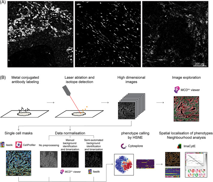
(A) CD163 expression patterns in three samples. A signal range of 3–20 mean dual counts was set for all images in the MCD viewer, but differences in signal intensity and background are observed between images. (B) Workflow for IMC FFPE imaging and data analysis, including the three tested data processing approaches where either no preprocessing, manual background identification and binarization or semi‐automated background identification and binarization were performed [Color figure can be viewed at wileyonlinelibrary.com]

First, we visualized immunodetection signal intensities, without normalization, per antibody, on all cell mask overlays where antibody signal was displayed as mean pixel intensity (Figure 2(A,B), lower panel). Where differences were observed, the original IMC images were inspected, showing that fluctuations in intensity on the cell masks generally corresponded to variations in signal to noise ratios. This resulted in either overestimation (Figure 2(A)) or underestimation (Figure 2(B)) of cells positive for a marker with variable signal to noise ratios between samples. Furthermore, alongside small differences in marker expression due to, for instance, signal spill over from neighboring cells, high variability in signal intensity between samples could potentially result in similar immune cell subsets being assigned to distinct immune cell populations when using automated clustering approaches. To test this, a t‐SNE embedding was computed using the single cell maker expression data extracted from 48 images. The embedding contained 393,727 cells and was visualized in a two‐dimensional scatterplot with sample IDs and expression of each marker shown by color coding. It was observed that cells with a similar marker profile were scattered throughout the t‐SNE embedding rather than clustering together (Figure 3(A), Figures S1 and S2(A)). Furthermore, cells also tended to group according to their sample of origin. These observations led to the hypothesis that the intensity range and signal to noise variation between samples can overshadow cell type differences and similarities. Finally, cells positive for FOXP3, CD20, or CD103, markers with a low signal to noise ratio, did not form groups in the t‐SNE analysis (Figure S1).

FIGURE 2.

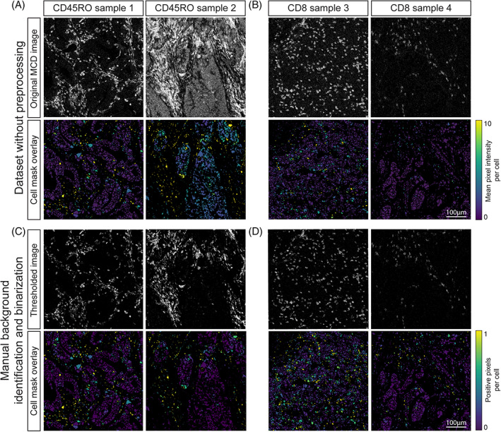
(A) Comparison between original MCD image and cell expression after mask overlay. Variation between images occurs due to differences in background as seen for CD45RO between sample 1 and 2 and (B) variation in signal intensity as observed for CD8 between sample 3 and 4. Signal in the cell mask ranged from 0–10 mean duals. (C) Comparison of CD45RO and (D) CD8 immunodetection in two thresholded MCD images and the mask overlay after manual thresholding and pixel binarization. Signal intensity ranges between 0 and 1 due to the visualization as relative frequency of positive pixels per cell [Color figure can be viewed at wileyonlinelibrary.com]

FIGURE 3.

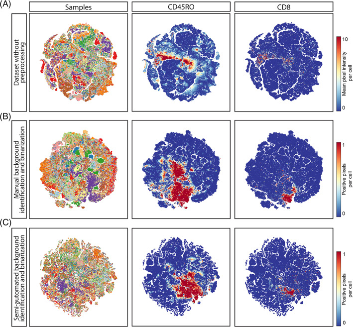
(A) T‐SNE analysis embedding of single cell data extracted from all 48 images without preprocessing. Each dot marks a cell and is colored by sample of origin.To determine the effect of data normalization, t‐SNE analysis embeddings were generated for the same dataset after (B) manual background identification and binarization and after (C) semi‐automated identification and binarization [Color figure can be viewed at wileyonlinelibrary.com]

3.2. Manual background identification and binarization normalizes IMC inter‐sample variation for automated downstream analysis

A methodology was devised to test whether the observed immunodetection variation could be overcome by normalizing the IMC data, while minimizing data loss, for downstream analysis. This approach utilized a user‐defined minimum signal threshold for each marker followed by pixel binarization of the dataset. To confirm whether this approach was sufficient for reliable downstream analysis, we visualized the percentage of positive pixels on the cell masks. Indeed, setting a minimum signal threshold overcame the variation between samples (Figure 2(C,D)), compared to images obtained without preprocessing of the data (Figure 2(A,B)) However, for markers with a low signal to noise ratio, it was observed that implementing a threshold not only filtered out the background but also signal corresponding to cells expressing the marker of interest (Figure S3(A–C)).

To further assess the effect of thresholding and binarization on downstream analysis, t‐SNE embedding, as described in the previous section, was performed on the single cell data obtained after manual background identification and binarization(Figure 3(B), Figure S1). In contrast to the t‐SNE embedding of data without preprocessing, cells with a similar marker profile clustered together (as observed for CD8, Figure S1). Furthermore, the distinction between positive and negative cells for a specific marker was clearer (as observed for CD163, Figure S1). Sample specific clustering was largely resolved but some sample‐related bias remained (Figure S2(B)) Further inspection of the t‐SNE embedding showed that the cells in those clusters were keratin‐positive (a marker for epithelial cells) with varying combinations of HLA‐DR, Ki67, and CD15 expression, markers that are often differentially expressed between cancer cells, which could, in part, explain the sample‐specific clustering of the tumor cells (Figure S2(C,D)). In line with the observations made during visual inspection, low numbers of cells positive for dim markers were observed (for instance CD20, FOXP3, Figure S1), albeit higher than the number of positive cells observed in t‐SNE of the dataset without normalization (Figure 3(A,B), Figure S1). Thus, manual background identification and binarization of pixel intensity largely resolved sample‐specific clustering and allowed for comparison between samples, but did not resolve the presence of false negatives.

Although manual background identification was found to overcome some of the challenges of analyzing FFPE IMC data, its major disadvantages are that it is time consuming and subject to errors as it requires vast knowledge of the expected immunodetection patterns of each marker and high inter‐user variability is inevitable. Furthermore, while background identification through thresholding removes background noise, a portion of specific signal can be lost, particularly when the signal to noise ratio is low, resulting in false negatives. Therefore, we set out to investigate if an automated and unbiased approach could replace manual thresholding. We first visualized the pixel data in histograms for each marker to assess if pixel intensity was bimodally distributed in order to set an automatic threshold between negative and positive pixels. However, no bimodal distribution but a negative correlation between number of pixels and signal intensity was observed, possibly in part due to detector noise of the mass cytometer (Figure S3(D)). We then investigated whether grouping pixel intensities per cell after applying cell masks onto the images allowed the definition of a threshold that separated positive and negative signals for a given marker. Initially, we set the threshold value at 1 mean duals and regarded all cells above this value as positive for a marker. Then, we visualized the data on cell level by plotting the percentage of positive pixels within a cell (Figure S3(E)). Also, at cell level, no clear bimodal distribution was observed. Similarly, cut‐off threshold values between 2 and 5 resulted in similar distributions (Figure S3 (F,I)). Moreover, a threshold of 2,9 mean duals was comparable to the cut‐off chosen during manual thresholding but this could not be deduced from the cell‐based value distribution (Figure S3(C,G)). Thus, an automated approach to determine a precise cut‐off value could not be established. Furthermore, setting a single‐value threshold, as was also observed with manual thresholding, causes a trade‐off between the removal of background and low intensity true signal and does not overcome case‐specific background signal as was observed for some images and markers (e.g., CD45RO, Figure 2(A)).

3.3. Semi‐automated background identification limits loss of data and normalizes the images for downstream analysis of IMC data

To correct for both technical noise and sample‐specific background signal, a semi‐automated background identification approach based on ilastik's pixel classification algorithm was employed. First, outliers were removed by saturating all pixels below the 1st and above the 99th percentile. This slightly improved the signal to noise compared to raw images, due to the removal of the brightest pixels, but variation in signal intensities between samples remained (Figure S4) as well as background noise (Figure 4). Thus, percentile normalization alone was not sufficient to normalize the data. Next, pixels corresponding to either “background” or “signal” were labeled for each marker and used to train a random forest classifier in ilastik. After training on 12 images per marker (or 1 image per sample) the algorithm was applied to all images in the dataset, to create binary signal masks for each marker. Of note, the algorithm takes into account pixel intensity but also patterns of neighboring pixels, which could aid the identification of background without losing true signal. Comparison of the images without preprocessing, after percentile normalization, manual background identification or the semi‐automated background identification, showed that the latter approach could be successfully applied to retain true signal while removing a substantial amount of background noise (Figure 4). To further confirm the validity of this approach, a t‐SNE embedding was computed from the single cell data extracted from the binary signal masks (Figure 3(C), Figure S5). Inspection of sample and marker overlays on the t‐SNE embedding, using color‐coding, showed cells grouped by the percentage of positive pixels for each marker rather than per sample, similar to the manual thresholding (Figure 3(B)). Furthermore, the signal to noise ratio was higher and cells that were positive for low intensity markers, such as FOXP3 and CD103, were identified by the semi‐automated background removal in contrast to manual thresholding (Figures S1 and S5).

FIGURE 4.

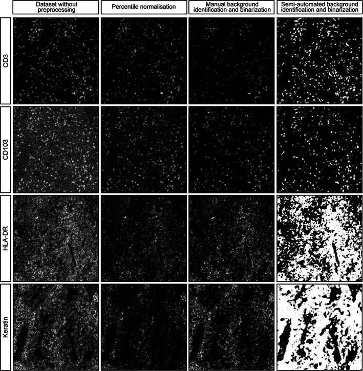
Representative images of CD3, CD103, HLA‐DR and keratin signal without preprocessing, percentile normalization, manual background removal or semi‐automated background removal, both followed by pixel binarization

3.4. Background removal and binarization combined with the proposed downstream analysis pipeline allows phenotyping of the tumor immune microenvironment

To demonstrate the added value of performing background identification and binarization of pixel intensity for the definition of immunophenotypes, clusters of cells with a comparable marker profile were identified, by applying Gaussian mean shift clustering on the t‐SNE embedding, computed in the previous section. Next, clusters were mapped back onto the segmentation masks in ImaCytE. A proliferating and nonproliferating tumor cluster was identified through the expression of keratin and distinguished by Ki‐67 (Figure 5(A)). Five myeloid clusters were identified by their CD68 expression and differentiated by CD204, CD163 and HLA‐DR expression. Furthermore, five lymphoid‐cell clusters could be identified where two clusters were CD8 positive, thus, corresponding to cytotoxic T cells. Of note, one of these clusters also showed positive signal for keratin indicating that these cells were located directly adjacent to epithelial cancer cells. Three clusters were CD8 negative and considered to be mostly composed of CD4 T cells. One of the clusters corresponded to regulatory T cells (FOXP3⁺) and the other two clusters were differentiated by Ki‐67 expression. The tumor, myeloid and lymphoid clusters were each mapped back onto the images and compared to the original MCD images in the MCD viewer (Figure 5(B)). Indeed, the number and location of positive cells for each phenotype was comparable between the images overlaid with phenotype masks and the original MCD images. Thus, semi‐automated background identification using ilastik combined with binarization is applicable to normalize IMC datasets derived from archival samples and allows for the identification and localization of biologically relevant phenotypes.

FIGURE 5.

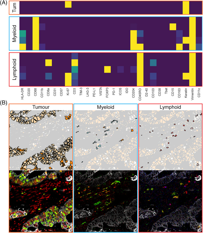
(A) Lymphoid, myeloid and tumor (tum) clusters identified in the t‐SNE analysis from Figure 3(C). (B) the clusters were mapped back onto a representative image and compared to their corresponding cell types in the MCD files. The images contain the following markers: For tumor keratin (white), Ki67 (green) and DNA (red), for myeloid cells CD68 (red) and CD163 (green) and for lymphoid cells CD3 (red), CD8 (green) and FOXP3 (blue). To improve visibility a lower threshold of 1 mean dual counts was set [Color figure can be viewed at wileyonlinelibrary.com]

4. DISCUSSION

With the rise of mass cytometry for the characterization of cellular contextures in health and disease, IMC has surfaced as a valuable tool to investigate immunophenotypes while preserving spatial information. IMC allows the simultaneous investigation of over 40 markers thereby generating complex datasets that require analysis tools that combine deep immunophenotyping data with spatial localization and neighborhood analysis. However, before data interpretation, nonbiological variation of signal intensities between tissues should be dealt with. Technical noise is consistent in each image and will therefore not influence downstream analysis as long as the signal to noise ratio is high, and can be addressed by optimizing the wet‐lab procedures and performing the immunodetection of tissues in a single experiment. However, sample‐specific background, related to tissue processing procedures, is impossible to address during the immunodetection procedures. FFPE tissue is often the tissue of choice for IMC due to its accessibility and good morphology. Differences in ischemia time, tissue fixation procedures, and age of the samples affects immunodetection and tissue‐related background, prompting the need to normalize the data before analysis. Furthermore, and in contrast to single cell technologies, spatial technologies, making use of tissue sections, require that cells are cut at different planes which influences the prevalence and intensity of a marker of interest. In light of this, it is preferable to classify cells into positive and negative categories for a given marker rather than relying excessively on intensity differences across cells for the identification of phenotypes.

Due to tissue‐specific variations in signal intensities, direct phenotyping of IMC data, without normalization, can lead to cells clustering per sample rather than phenotypes as the variation in overall signal intensity overshadows the differences between cell types. Furthermore, the signal range of the more abundant structural markers (e.g. keratin, vimentin) is much wider compared to scarcer, but important targets of investigation (e.g. co‐receptors on T cells). This difference influences downstream computational methods such as clustering or dimensionality reduction algorithms and hinders the detection of specific cell subsets.

In this work, we enable the analysis of large IMC datasets and improve the detection of cells expressing lowly abundant proteins by removing background noise and binarizing each sample's pixel values. Binarizing was done by assigning the value of 1 to all pixels determined to be positive for a given marker and the value of 0 to all other pixels. More specifically, we tested two different normalization approaches. First, a manual method was utilized where a minimum threshold corresponding to signal was set for each marker in all images. All pixels below threshold were set to 0 and all pixels above were set to 1. Then, marker expression per cell was defined as the percentage of positive pixels per cell. This approach indeed partially overcame variation between tissues and allowed for t‐SNE‐guided phenotype identification. However, manual thresholding is labor intensive and relies on vast knowledge of the expected immunodetection patterns for each antibody, leading to potentially biased results. In general, thresholding is a trade‐off between the removal of background and loss of true signal and therefore can result in the frequent designation of false negatives. An automated approach could overcome these challenges but large variations between samples and markers make fully automated unsupervised methods infeasible and the lack of labeled datasets is prohibitive for supervised machine learning approaches. Therefore, we propose a semi‐automated, methodology using ilastik where we first annotate representative pixels either as actual signal or background noise and then a random forest classifier is run to categorize the whole dataset, based on these categories. This approach is faster, less subjective, and results in data comparable to manual thresholding. Furthermore, loss of true signal is less frequently observed, and dim markers are more clearly represented after semi‐automated background identification and pixel intensity binarization. A drawback of signal binarization is the potential loss of information on biologically relevant, signal intensity variations for a given marker. However, it is currently challenging to distinguish between biological and technical causes for signal intensity variations in in situ imaging approaches that utilize FFPE tissue. Thus, to limit the loss of biologically relevant information, we chose to binarize the data at pixel level which still allows the evaluation of differences in number of positive pixels per cell. Finally, accurate cell segmentation remains an important challenge to address in molecular imaging. Current methodologies, like the ones employed here, are not fool proof, particularly in areas where cells are densely packed. Therefore, we have performed cell segmentation on raw images and upstream of normalization approaches in order to allow their comparison independently of segmentation.

In recent years, great advancements have been made in the analysis and interpretation of single cell (mass cytometry) data and a number of developed tools have also proven useful for the analysis of IMC datasets. However, it is essential that such knowledge is combined with the accumulated experience in the immunohistochemistry and imaging fields to best address immunodetection variation among samples and to deal with technical artifacts. The here described normalization methodology enables the comparative analysis of datasets generated from different tissues and it supports the identification of less abundant cellular subsets. Furthermore, the methodology does not require adaptation in immunodetection procedure and can, thus, be directly applied on available datasets. In sum, this work has the potential to directly aid research groups in their analysis and interpretation of imaging mass cytometry data.

AUTHOR CONTRIBUTIONS

Marieke Ijsselsteijn: Investigation; methodology; validation; visualization; writing‐original draft. Antonios Somarakis: Funding acquisition; investigation; software; validation; visualization; writing‐original draft. Boudewijn Lelieveldt: Supervision. Thomas Höllt: Software; supervision; writing‐review & editing. Noel de Miranda: Conceptualization; funding acquisition; supervision; writing‐review & editing.

CONFLICT OF INTEREST

The authors declare no conflicts of interest.

Supporting information

Table S1. Imaging mass cytometry antibody panel. Antibodies with a * had prediluted stock solutions

Figure S1.| t‐SNE analysis on single cells extracted from dataset without preprocessing and the dataset generated with manual background identification and binarization.

Figure S2.| (A) t‐SNE embedding of single cell data extracted from dataset without pre‐processing. Each color represents a different sample and cells cluster together by phenotype. Sample‐specific clustering is encircled. (B) t‐SNE embedding of single cell data extracted from dataset generated with manual background identification and binarization. Each color represents a different sample and sample specific clustering is encircled. (C,D) Keratin, Ki67, CD15, and HLA‐DR expression overlay on the t‐SNE from data without pre‐processing (C) and data that underwent manual background identification and binarization (D).

Figure S3.| (A–C) CD3 expression in a representative image with a pixel threshold of 0, 1, or 2,9. (D) pixel data plotted in a histogram displaying the relation between pixel intensity (x‐axis) and frequency (y‐axis). (E) Mean CD3 positive pixels per cell with a cut off threshold at 1. All pixels below threshold were set to 0 and above threshold at 1 and used to determine the mean intensity per cell. (F‐I) histograms of CD3 expression with different threshold between 2 and 5.

Figure S4.|CD163 expression pattern in the three samples after saturation of pixels below the 1st and above the 99th percentile.

Figure S5.| t‐SNE analysis on single cells extracted from the dataset generated through semi‐automated background identification and binarization. Data is shown in a range of 0 (blue) to 1 (red).

MIFlowCyt MIFlowCyt Item Checklist.

Ijsselsteijn ME, Somarakis A, Lelieveldt BPF, Höllt T, de Miranda NFCC. Semi‐automated background removal limits data loss and normalizes imaging mass cytometry data. Cytometry. 2021;99:1187–1197. 10.1002/cyto.a.24480

REFERENCES

- 1. de Vries NL, van Unen V, Ijsselsteijn ME, Abdelaal T, van der Breggen R, Farina Sarasqueta A, et al. High‐dimensional cytometric analysis of colorectal cancer reveals novel mediators of antitumour immunity. Gut. 2020;69:691–703. [DOI] [PMC free article] [PubMed] [Google Scholar]
- 2. Rubin SJS, Bai L, Haileselassie Y, Garay G, Yun C, Becker L, et al. Mass cytometry reveals systemic and local immune signatures that distinguish inflammatory bowel diseases. Nat Commun. 2019;10:2686. [DOI] [PMC free article] [PubMed] [Google Scholar]
- 3. Li N, van Unen V, Abdelaal T, Guo N, Kasatskaya SA, Ladell K, et al. Memory CD4(+) T cells are generated in the human fetal intestine. Nat Immunol. 2019;20:301–12. [DOI] [PMC free article] [PubMed] [Google Scholar]
- 4. Bendall SC, Simonds EF, Qiu P, Amir ED, Krutzik PO, Finck R, et al. Single‐cell mass cytometry of differential immune and drug responses across a human hematopoietic continuum. Science. 2011;332:687–96. [DOI] [PMC free article] [PubMed] [Google Scholar]
- 5. Newell EW, Sigal N, Bendall SC, Nolan GP, Davis MM. Cytometry by time‐of‐flight shows combinatorial cytokine expression and virus‐specific cell niches within a continuum of CD8+ T cell phenotypes. Immunity. 2012;36:142–52. [DOI] [PMC free article] [PubMed] [Google Scholar]
- 6. Wei SC, Levine JH, Cogdill AP, Zhao Y, Anang NAS, Andrews MC, et al. Distinct cellular mechanisms underlie anti‐CTLA‐4 and anti‐PD‐1 checkpoint blockade. Cell. 2017;170:1120–33. e17. [DOI] [PMC free article] [PubMed] [Google Scholar]
- 7. Bandura DR, Baranov VI, Ornatsky OI, Antonov A, Kinach R, Lou X, et al. Mass cytometry: technique for real time single cell multitarget immunoassay based on inductively coupled plasma time‐of‐flight mass spectrometry. Anal Chem. 2009;81:6813–22. [DOI] [PubMed] [Google Scholar]
- 8. Ornatsky OI, Kinach R, Bandura DR, Lou X, Tanner SD, Baranov VI, et al. Development of analytical methods for multiplex bio‐assay with inductively coupled plasma mass spectrometry. J Anal At Spectrom. 2008;23:463–9. [DOI] [PMC free article] [PubMed] [Google Scholar]
- 9. Giesen C, Wang HA, Schapiro D, Zivanovic N, Jacobs A, Hattendorf B, et al. Highly multiplexed imaging of tumor tissues with subcellular resolution by mass cytometry. Nat Methods. 2014;11:417–22. [DOI] [PubMed] [Google Scholar]
- 10. Chevrier S, Crowell HL, Zanotelli VRT, Engler S, Robinson MD, Bodenmiller B. Compensation of signal spillover in suspension and imaging mass Cytometry. Cell Syst. 2018;6:612–20. [DOI] [PMC free article] [PubMed] [Google Scholar]
- 11. Ijsselsteijn ME, van der Breggen R, Farina Sarasqueta A, Koning F, de Miranda N. A 40‐marker panel for high dimensional characterization of cancer immune microenvironments by imaging mass Cytometry. Front Immunol. 2019;10:2534. [DOI] [PMC free article] [PubMed] [Google Scholar]
- 12. Guo N, van Unen V, Ijsselsteijn ME, Ouboter LF, van der Meulen AE, Chuva de Sousa Lopes SM, et al. A 34‐marker panel for imaging mass cytometric analysis of human snap‐frozen tissue. Front Immunol. 2020;11:1466. [DOI] [PMC free article] [PubMed] [Google Scholar]
- 13. Schulz D, Zanotelli VRT, Fischer JR, Schapiro D, Engler S, Lun XK, et al. Simultaneous multiplexed imaging of mRNA and proteins with subcellular resolution in breast cancer tissue samples by mass cytometry. Cell Syst. 2018;6:531. [DOI] [PMC free article] [PubMed] [Google Scholar]
- 14. Jackson HW, Fischer JR, Zanotelli VRT, Ali HR, Mechera R, Soysal SD, et al. The single‐cell pathology landscape of breast cancer. Nature. 2020;578:615–20. [DOI] [PubMed] [Google Scholar]
- 15. Wang YJ, Traum D, Schug J, Gao L, Liu C, Consortium H, et al. Multiplexed in situ imaging mass Cytometry analysis of the human endocrine pancreas and immune system in type 1 diabetes. Cell Metab. 2019;29:769–83. [DOI] [PMC free article] [PubMed] [Google Scholar]
- 16. Damond N, Engler S, Zanotelli VRT, Schapiro D, Wasserfall CH, Kusmartseva I, et al. A map of human type 1 diabetes progression by imaging mass Cytometry. Cell Metab. 2019;29:755–68. [DOI] [PMC free article] [PubMed] [Google Scholar]
- 17. Berg S, Kutra D, Kroeger T, Straehle CN, Kausler BX, Haubold C, et al. Ilastik: interactive machine learning for (bio)image analysis. Nat Methods. 2019;16:1226–32. [DOI] [PubMed] [Google Scholar]
- 18. Carpenter AE, Jones TR, Lamprecht MR, Clarke C, Kang IH, Friman O, et al. CellProfiler: image analysis software for identifying and quantifying cell phenotypes. Genome Biol. 2006;7:R100. [DOI] [PMC free article] [PubMed] [Google Scholar]
- 19. Schapiro D, Jackson HW, Raghuraman S, Fischer JR, Zanotelli VRT, Schulz D, et al. histoCAT: analysis of cell phenotypes and interactions in multiplex image cytometry data. Nat Methods. 2017;14:873–6. [DOI] [PMC free article] [PubMed] [Google Scholar]
- 20. Somarakis A, Van Unen V, Koning F, Lelieveldt BPF, Hollt T. ImaCytE: visual exploration of cellular microenvironments for imaging mass cytometry data. IEEE Trans Vis Comput Graph. 2019;27(1):98‐110. [DOI] [PubMed] [Google Scholar]
- 21. Economou M, Schoni L, Hammer C, Galvan JA, Mueller DE, Zlobec I. Proper paraffin slide storage is crucial for translational research projects involving immunohistochemistry stains. Clin Transl Med. 2014;3:4. [DOI] [PMC free article] [PubMed] [Google Scholar]
- 22. Werner M, Chott A, Fabiano A, Battifora H. Effect of formalin tissue fixation and processing on immunohistochemistry. Am J Surg Pathol. 2000;24:1016–9. [DOI] [PubMed] [Google Scholar]
- 23. O'Hurley G, Sjöstedt E, Rahman A, Li B, Kampf C, Pontén F, et al. Garbage in, garbage out: a critical evaluation of strategies used for validation of immunohistochemical biomarkers. Mol Oncol. 2014;8:783–98. [DOI] [PMC free article] [PubMed] [Google Scholar]
- 24. Bussolati G, Leonardo E. Technical pitfalls potentially affecting diagnoses in immunohistochemistry. J Clin Pathol. 2008;61:1184–92. [DOI] [PubMed] [Google Scholar]
- 25. Taylor CR, Levenson RM. Quantification of immunohistochemistry–issues concerning methods, utility and semiquantitative assessment II. Histopathology. 2006;49:411–24. [DOI] [PubMed] [Google Scholar]
- 26. Leong AS. Quantitation in immunohistology: fact or fiction? A discussion of variables that influence results. Appl Immunohistochem Mol Morphol. 2004;12:1–7. [DOI] [PubMed] [Google Scholar]
- 27. van Unen V, Hollt T, Pezzotti N, Li N, Reinders MJT, Eisemann E, et al. Visual analysis of mass cytometry data by hierarchical stochastic neighbour embedding reveals rare cell types. Nat Commun. 2017;8:1740. [DOI] [PMC free article] [PubMed] [Google Scholar]
- 28. Höllt T, Pezzotti N, van Unen V, Koning F, Eisemann E, Lelieveldt B, et al. Cytosplore: interactive immune cell Phenotyping for large single‐cell datasets. Computer Graphics Forum. 2016;35:171–80. [Google Scholar]
Associated Data
This section collects any data citations, data availability statements, or supplementary materials included in this article.
Supplementary Materials