

Abstract
Because the diffusivity of particles undergoing the Brownian motion is inversely proportional to their sizes, the size distribution of submicron particles can be estimated by tracking their movement. This particle tracking analysis (PTA) has been applied in various fields, but mainly focused on resolving monodispersed particle populations and is rarely used for measuring oceanic particles that are naturally polydispersed. We demonstrated using Monte Carlo simulation that, in principle, PTA can be used to size natural, oceanic particles. We conducted a series of lab experiments using microbeads of NIST‐traceable sizes to evaluate the performance of ViewSizer 3000, a PTA‐based commercial instrument, and found two major uncertainties: (1) the sample volume varies with the size of particles and (2) the signal‐to‐noise ratio for particles of sizes < 200–250 nm was reduced and hence their concentration was underestimated with the presence of larger particles. After applying the volume correction, we found the instrument can resolve oceanic submicron particles of sizes greater than 250 nm with a mean absolute error of 3.9% in size and 38% in concentration.
Submicron particles of sizes from 0.1 to 1 μm include various types of particulate matter in seawater, such as viruses, bacteria, pico‐size phytoplankton and minerogenic clay, etc. (Koike et al. 1990, Guo and Santschi 1997, Wells 1998, Stramski et al. 2004, Filella 2006, Jonasz and Fournier 2007). Although particles size distributions (PSDs) in seawater have been measured for decades (Sheldon et al. 1972, Jonasz 1983, McCave 1984, Jackson et al. 1997, Jackson and Checkley 2011), due to the limitation in technology, only a few studies reported measurements of PSDs in this submicron size range.
Using ultracentrifugation and transmission electron microscope, Wells and Goldberg (1991, 1992, 1994) measured submicron particles in the coastal water off California and in the Southern Ocean. This method requires hours of operation for the ultracentrifugation and is only applicable for particles of sizes < 0.2 μm (Wells and Goldberg 1992). Groundwater et al. (2012) developed a technique utilizing a scanning electron microscope (SEM) coupled with an energy‐dispersive spectrometer and image processing to measure submicron particles. Although SEM is capable of achieving nanometer resolution, the focus of Groundwater et al. (2012) was for sizes greater than 1 μm. Using commercial instruments Elzone Particle Size Analyzer and/or the Multisizer Coulter Counter, Koike et al. (1990), Longhurst et al. (1992), and Yamasaki et al. (1998) measured submicron particles in various locations. Both Elzone Particle Size Analyzer and Multisizer Coulter Counter are based on the relation between the volume of a particle and its electrical resistance, and the inherent electronic noise limits the detection size to greater than 0.38 μm (Koike et al. 1990, Longhurst et al. 1992). Vaillancourt and Balch (2000) applied the flow field‐flow fraction technique to size oceanic particles. This technique has the ability to identify particles from ~ 4 nm to a few microns, but the concentrations of particles need to be calibrated by other methods. The preconcentration process and the mass loss during the measurement (up to 50%) also limits the oceanic applications of this technique (Hassellöv and Kaegi 2009, Baalousha et al. 2011). Ackleson and Spinrad (1988) and Green et al. (2003) combined flow cytometry with Mie theory to infer particle diameter and refractive index from light scattering measured at several angles. Recent tests in the natural environment show the method can resolve particles within 0.5–10 μm size range (Agagliate et al. 2018). However, this technique assumes particles are homogeneous spheres, which could lead to significant errors (Zhao et al. 2020).
Gallego‐Urrea et al. (2010) and Gondikas et al. (2020) measured submicron particles in Swedish coastal waters using a particle tracking instrument, NanoSight developed by Malloy and Carr (2006). This instrument applies particle tracking analysis (PTA) based on the Brownian motion, where the diffusivity of a particle is inversely related to the size of this particle, a phenomenon first deduced by Einstein (1905). This technique has been developed for decades in various fields and applied with different configurations (Geerts et al. 1987, Gelles et al. 1988, Ren et al. 1996, Gallego‐Urrea et al. 2011, Anderson et al. 2013, McElfresh et al. 2018). The NanoSight uses one laser beam to illuminate a sample of particles and takes a series of images of particles undergoing the Brownian motion. By subsequent image analysis, the motion of each particle is tracked and analyzed for traveling distance. The PTA technique has the potential to measure the PSDs of submicron particles rapidly with few assumptions (Geerts et al. 1987, Malloy and Carr 2006).
Despite its potential, PTA has been seldom applied to measure PSDs of oceanic particles. A major hurdle for oceanic applications is that PTA relies on the intensity of the scattered light to identify particles and for smaller submicron particles the scattering intensity of a particle is proportional to the 6th power of the size of the particle. For example, the scattering intensity by a 100 nm particle is only 1/64th of that by a 200 nm particle. Consequently, when applying PTA to oceanic particles under the same illumination, smaller particles are often too dim to be seen. Stramski et al. (2017) proposed to use three laser beams of different wavelengths for illumination. Because the scattering intensity of a particle is inversely proportional to the 4th power of the wavelength, the difference in scattered intensity caused by the particle sizes is compensated by the difference in the wavelength. Continuing with the previous example, the intensity scattered by the 100 nm particle illuminated by light of wavelength 450 nm is 1/13th of that by the 200 nm particle illuminated by light of wavelength 650 nm. The technique proposed by Stramski et al. (2017) has been commercialized as a product called ViewSizer 3000, with one of its intended applications being to quantify natural submicron populations, including oceanic, colloidal particles.
McElfresh et al. (2018) tested a ViewSizer 3000 with gold particle populations of mean diameters ranging from 50 to 250 nm and polystyrene latex bead populations of mean diameters ranging from 78 to 262 nm. They found ViewSizer 3000 could correctly detect the mean sizes of these artificial samples. Despite its designed intention, ViewSizer 3000 has not been tested for oceanic particles, which leads to the goal of this study. The objective of this study is threefold. First, we investigate the inherent uncertainty of applying the PTA technique to size particles. Second, we examine if the technique is suitable for polydispersed populations such as oceanic particles. Finally, we quantify the instrument uncertainties associated with ViewSizer 3000. Our study will help to better understand the application of the Brownian motion tracking technique to derive the size distribution of submicron particles in the oceans.
In the following, we will first use Monte Carlo simulation to illustrate the working theory and the inherent uncertainties of the PTA technique and to demonstrate that PTA can quantify naturally occurring particles. We will then investigate the uncertainties of ViewSizer 3000 in deriving the particle size distribution and propose the corrections. Finally, we will test the proposed corrections using the field measurements.
Background and theory
Theory of PTA
For particles undergoing Brownian motion, the diffusivity of the particles (D, m2 s−1) is inversely proportional to their hydrodynamic diameter following the Einstein–Langevin equation (Einstein 1905, Langevin 1908):
| (1) |
where k B is the Boltzmann constant (1.38064852 × 10⁻²³ J K−1), K T the absolute temperature (K), η the dynamic viscosity of the liquid (N s m−2), and d the hydrodynamic diameter of the particle, also known as the Stokes–Einstein diameter, which represents the equivalent diameter of a sphere that would undergo the same Brownian motion as the particle in the same liquid. As a particle going through Brownian motion, the probability of the distance (r) that the particle moves over a time interval ΔT follows normal distribution with mean distance being zero. In one dimension, Einstein (1905) showed the variance of the traveling distance:
| (2) |
In Eq. 2, r 1 signifies that the distance is measured in one dimension. As the Brownian motion in each dimension is independent, the variance of Brownian motion in two‐dimension or three‐dimension are additive (Crank 1975, Hiemenz and Rajagopalan 1997):
| (3) |
| (4) |
In principle, if n (n > 1) locations of a particle (x i, y i, z i) are tracked at ΔT interval, the variance of r can also be approximated by the mean square of displacement (MSD). In one, two or three‐dimensions:
| (5) |
| (6) |
| (7) |
The diffusivity of the particle (D), hence the hydrodynamic diameter of the particle (d), can be easily solved using the estimated MSD to approximate the true variance of Brownian motion in the corresponding dimension.
Monte Carlo simulation of the Brownian motion
To demonstrate the PTA technique, we simulated Brownian motion for particles of different sizes following Anger and Prescott (1970). The particle's movements are simulated independently in each of the three‐dimensions:
| (8) |
Here, represents the sequence of the particle's positions; Δt (s) is the time interval at which a new position is simulated; P is a random number generated from the standard normal distribution; and D is calculated according to Eq. 1 using dynamic viscosity of pure water at 25°C (η ≈ 8.9 × 10⁻⁴ N s m−2). The starting point of each simulation, which is not important, is set at . Padding and Louis (2006) investigated different time scales to properly simulate various physical processes involved in Brownian motion. For our simulation, we set Δt = 1/30 s and simulated N = 301 positions for a total of 10 s based on the frame rate of the camera used in the ViewSizer 3000. Figure 1 shows the trajectories simulated in three‐dimension for three particles of sizes 100, 300, and 900 nm, and their two‐dimensional projections to the X–Y, Y–Z, and Z–X planes. Both two‐dimensional and three‐dimensional trajectories show that smaller particles meander over greater range than larger particles, which is expected.
Fig. 1.

The Brownian motion simulated for 10 s with a 1/30 s interval for 3 particles of sizes 100, 300, and 900 nm. The darker curves are the particle trajectories in three‐dimension and the brighter curves are their two‐dimensional projections onto X–Y, Y–Z, and Z–X planes.
Working theory of PTA
Generally, movement of particles is tracked and analyzed through an imaging system that samples at a regular interval. When particles going through three‐dimensional random motion are tracked through two‐dimensional imaging system, the two‐dimensional equation (Eq. 3) for calculating particle diffusivity should be used (Geerts et al. 1987, Qian et al. 1991).
Here, we use the three particles in Fig. 1 to illustrate how diffusivity D is generally estimated with an imaging system. Assuming 301 images are taken, by comparing every pair of images in sequence (1, 2; 2, 3; 3, 4… for a total of 300 pairs), we can calculate MSDs for each particle using Eq. 6. These MSDs correspond to a time interval ΔT = 1 × Δt = 1/30 s. We then compare every other image in sequence (1, 3; 2, 4; 3, 5… for a total of 299 pairs) and calculate MSDs for each particle. These MSDs correspond to ΔT = 2 × Δt = 1/15 s. Repeating this process, a series of MSDs can be calculated for each particle that correspond to an increasing ΔT. Figure 2 shows the MSDs calculated with various ΔT values for each of the three particles. Note that we simulated the Brownian motion in three‐dimensions (x, y, z) but in calculating MSDs for Fig. 2, we only used (x, y) locations to emulate the two‐dimensional imaging. Apparently, MSDs vs. ΔT curves have different inclinations for particle of different sizes. Ideally, these curves should be linear with a slope of values equal to 4D (Eq. 3). Statistically, within a fixed sampling period (10 s in our case) a smaller ΔT provides more data points to estimate MSD and hence reduces the uncertainties; but in practice, if ΔT is too small, the distance of Brownian motion, especially for larger particles, might be too small to be estimated accurately. On the other hand, a larger ΔT would limit the number of data used to estimate the MSD, and hence increases the uncertainty. This is clearly shown in Fig. 2, where the MSDs corresponding to larger ΔT deviate increasingly from the line. Overall, MSD and hence the size of particles can be better estimated with smaller ΔT values.
Fig. 2.
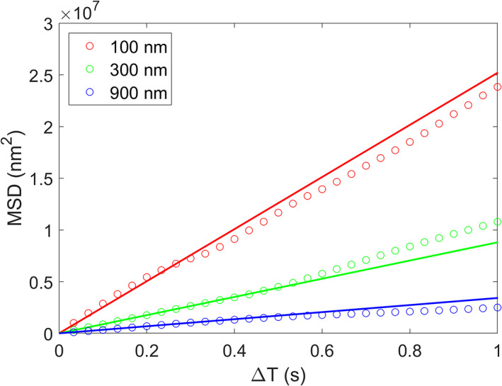
The MSDs calculated for three particles shown in Fig. 1 with different ΔT values. The solid lines have slopes of values = 4D (Eq. 3).
Inherent uncertainty of PTA
To evaluate the uncertainty of PTA, we repeated the simulation shown in Fig. 1 for five sizes (100, 300, 500, 700, and 900 nm) and compared the derived size distributions with their corresponding input sizes (Fig. 3a). The input size distribution is uniform and for each size 5 × 10⁵ particles were generated. First, we derived PSDs using the particle positions separated by ΔT = 1/30 s in both three‐dimensional (gray curves in Fig. 3a) and two‐dimensional (red curves in Fig. 3a) settings. Instead of uniform distribution, the derived PSDs appear to be broadened into a normal distribution, but with the mean values the same as the inputs. This suggests that PTA has an inherent uncertainty in resolving the size. We use coefficients of variation (CV; standard deviation divided by mean value) to represent this inherent uncertainty and their values are shown in Fig. 3b. The PSDs derived in three‐dimension with ΔT = 1/30 s have ~ 5% CV regardless of the size (gray dots in Fig. 3b) and the PSDs derived in two‐dimension with ΔT = 1/30 s are slightly broader with ~ 6% CV (red dots in Fig. 3b). A further test in two‐dimension with ΔT = 1/6 s shows an even greater CV of ~ 13% (blue dots in Fig. 3b). In this Monte Carlo simulation, each position was simulated at an interval of 1/30 s, therefore ΔT = 1/30 s was the smallest interval we can use to estimate PSD. We also tested simulation with smaller intervals at 1/50 s and 1/100 s, for which the estimated PSDs are still normally distributed but with CVs smaller than that with ΔT = 1/30 s (results not shown).
Fig. 3.

(a) Comparison of PSDs between the input values (black lines) and those derived from PTA (colored curves) using four different approaches: Three‐dimension direct estimate with ΔT = 1/30 s, two‐dimension direct estimate with ΔT = 1/30 s, two‐dimension direct estimate with ΔT = 1/6 s, and two‐dimension regression over ΔT = 1/30–1/6 s. See text for details. (b) The coefficients of variation estimated for the derived PSDs.
In practical applications with an imaging system, a particle going through three‐dimensional random motion does not always appear in every two‐dimensional image. This could happen for a variety of reasons, including but not limited to out‐of‐focus, blocking by another particle, etc. When this happens, the pairing of particles in two consecutive images is disrupted. To overcome this issue and to reduce the uncertainty, the slopes of MSD vs. ΔT (i.e., the diffusivity) in Fig. 2 are often estimated through linear regression using MSD values estimated at multiple ΔT's (Qian et al. 1991). To ensure physical soundness, the regression is forced through the origin, i.e., when the sampling interval approaches zero, the movement of particles approaches zero. We tested this approach to estimate the sizes using the linear regression over a range of ΔT values, 1/30–1/6 s (green curves in Fig. 3a). The PSDs estimated using linear regression over a range of ΔT values from 1/30 to 1/6 s have the same mean size as the inputs but with a CV value of approximately 10% (green dots in Fig. 3b), which lies between the CV values estimated directly with ΔT = 1/30 s (red dots) and ΔT = 1/6 s (blue dots). Qian et al. (1991) analytically derived an error budget for the PTA, which predicts an error of 10.6% for the case we tested here (ΔT = 1/30–1/6 s, green curve in Fig. 3a). Our uncertainty of ~ 10% (green dots in Fig. 3b) is consistent with this theoretical prediction. To further reduce the uncertainty, Saxton (1997) suggested a weighted regression to estimate the diffusivity with weighting decreasing with increasing time interval. Berglund (2010) and Michalet and Berglund (2012) developed a method to choose the optimal number of ΔT and the sampling period. This method essentially used an iterative search to find the optimal values for ΔT and the sampling period for linear regression to meet the expected precisions for estimating the diffusivity.
Overall, the PTA approach can estimate the mean size of particles very well with an uncertainty depending on the exact implementation of the technique. The root of the uncertainty lies in the stochastic nature of the Brownian motions (Chandrasekhar 1943, Qian et al. 1991), where the variance of movements of particles in Brownian motion is estimated in one‐, two‐, or three‐dimension (Eqs. (5), (6), (7)) to approximate the true variance in three‐dimension. Based on our results, the uncertainty at the same sampling interval only increased slightly from three‐dimension sampling to two‐dimension sampling. Increased sampling interval leads to greater uncertainty, which, however, can be alleviated with the regression approach.
Additional Monte Carlo simulation was performed for particles following the normal distribution to approximate particles that are distributed in a narrow size range. The mean diameters of the particles are 100, 303, 508, 702, and 903 nm and the standard deviations are 7.8, 4.7, 8.5, 4.9, and 4.1 nm, respectively. These size parameters were taken from the polystyrene latex beads of NIST‐traceable sizes that we used later to evaluate ViewSizer 3000. For each size, 5 × 10⁵ particles were generated. We used the same set of approaches as mentioned above to estimate the size distributions, which were then compared with the input distributions (Fig. 4). The derived PSDs are also normally distributed with the same mean values as the inputs but with greater standard deviations, suggesting that for narrowly distributed particles, PTA also introduces additional uncertainty. Comparison of Fig. 4 with Fig. 3a indicates that the same uncertainty pattern observed for uniformly distributed particles also applies to the narrowly distributed particles, i.e., the uncertainty increases from three‐dimensional sampling to two‐dimensional sampling and increases with increasing sampling interval ΔT.
Fig. 4.

Same as Fig. 3a but for input PSDs of normal distribution.
Application of PTA to naturally occurring particles
To evaluate if PTA can be applied to measure natural particles which exist in a continuum of sizes, we performed another Monte Carlo simulation with the input particles following power‐law distribution of three different slopes (−3, −4, and −5) to approximate the PSD of natural particles in the oceans (Junge 1969, Wells and Goldberg 1994, Filella 2006, Jonasz and Fournier 2007). For each slope value, 1 × 10⁶ particles were generated of sizes between 100 and 1000 nm.
Again, we used the same approaches as in Fig. 3 to estimate the size and compared the estimated PSDs with the inputs (Fig. 5). The derived PSDs are also broader than the inputs, but the broadening only occurs near the two ends, < 120 and > 900 nm (Fig. 5). The broadening near the two ends follows the same pattern as observed for uniformly (Fig. 3) and normally (Fig. 4) distributed particles. Between the two ends, however, the derived PSDs align well with the inputs, suggesting that the broadening observed for particles at individual sizes (Fig. 3a) or over a narrow size range (Fig. 4) compensates each other in this continuously distributed size spectrum. Between 120 and 900 nm, derived PSDs agree with the inputs with a correlation coefficient of 0.98 and a mean absolute difference < 3%. The PSDs shown in Fig. 5 suggests that the PTA can be used to size natural particles that typically exhibit a continuum in size distributions by tracking the Brownian motion in two‐dimension.
Fig. 5.

Same as Fig. 3a but for input PSDs of power‐law distribution with slopes = −3 (a), −4 (b), and −5 (c).
Materials and procedures
ViewSizer 3000
ViewSizer 3000 deploys three laser beams at 450, 520, and 650 nm illuminating a cuvette that holds samples. Scattered light at 90° relative to the incident beam is recorded by a CCD sensor with a Byer color filter. The cuvette is placed in a container painted black to minimize the stray light. An insert, also painted black, is placed inside the cuvette to further minimize the stray light (Fig. 6). The focal plane is inside the insert and has an area of 288 μm × 162 μm. The average depth of field is 52 μm, giving an average sampling volume V = 2.42 × 10⁻⁶ mL. For comparison, the entire cuvette has a volume of approximately 3 mL. The actual depth of field varies slightly with the intensity of the scattered light, which can be affected by the size, shape and refractive index by the particles (Gallego‐Urrea et al. 2014). For instance, the larger (smaller) the size of a particle is, the greater (less) the intensity of the scattered light, and hence the farther away (closer) from the CCD the particle can be located that still produces sufficient contrast to be identified in images. Similarly, the greater the refractive index is, the greater the intensity of the scattered light but with relatively smaller effect than size (the scattering intensity increases by a factor of ~ 20 for particles in water with the relative refractive index between 1.04 and 1.18 whereas intensity increases by a factor of ~ 3000 for particles of sizes between 100 and 900 nm). The exact variation of the depth of field depends on the sensitivity of the CCD sensor and is specific to the instrument. The variation of the depth of field does not affect the estimate of the size of particles but affects the sampling volume and hence the estimate of the concentration of particles.
Fig. 6.

Picture of a ViewSizer 3000 (left) showing the approximate location of the cuvette with a black insert inside (middle). Three laser beams (450, 520, and 650 nm) illuminate the sample inside the insert simultaneously and an imaging system record the scattered light at 90° relative to the incident light. The black diagram on the right shows the location and dimension of the focal plane, which has an area of 288 μm × 162 μm. The depth of field varies slightly with the size of particles, averaging 52 μm.
ViewSizer 3000 records videos and estimates the size of each particle by analyzing the recorded positions of the particle according to the principle described in the previous sections. The detailed process is proprietary. By knowing the sizes of all particles recorded, the PSDs can be generated by summing the count of particles within each size bin and normalizing the total number of particles in each size bin by the sampling volume corresponding to this size bin.
Lab measurement of polystyrene latex beads
ViewSizer 3000 has not been used for quantifying particles in the oceans and therefore its performance for quantifying naturally occurring particles needs to be evaluated. We conducted lab experiments using polystyrene latex beads of NIST‐traceable sizes to evaluate its performance and its uncertainty. The beads used are in nine nominal sizes, whose mean diameters are 100, 152, 203, 303, 400, 508, 600, 702, and 903 nm. Each of these bead populations follows a normal distribution and their standard deviations are 7.8, 5.0, 5.3, 4.7, 7.3, 8.5, 10.0, 4.9, and 4.1 nm, respectively.
Two general types of bead solutions were prepared: a monodispersed solution has beads of one nominal size and a polydispersed solution has beads of several different nominal sizes. The monodispersed solutions are mainly used to evaluate and calibrate the performance of ViewSizer 3000. As mentioned earlier, the actual sampling volume varies with the size of particles, a size‐dependent volume correction factor was determined with monodispersed solutions. Polydispersed solutions are mainly used for validation. Even though polydispersed bead populations cannot exactly represent the size distribution for the oceanic particles that typically exist in a continuum of sizes, they are the closest approximation to evaluate ViewSizer 3000's capability to measure oceanic particles.
During the lab measurements, all glass containers were bathed in diluted hydrochloride acid (1 M) overnight then rinsed with the ultrapure water at least six times. Ultrapure water was produced by a Direct‐Q 3 UV water purification system (DQ3). Monodispersed bead solutions were prepared at concentrations between 1 × 10⁶ and 5 × 10⁷ mL−1 and polydispersed bead solutions were prepared with various monodispersed bead solutions with total concentrations between 2.5 × 10⁶ and 2 × 10⁷ mL−1. These concentrations are similar to the concentrations of natural submicron particles in seawater that have been measured (Koike et al. 1990, Longhurst et al. 1992, Yamasaki et al. 1998, Gallego‐Urrea et al. 2010). Before each measurement, the quartz cuvette and the insert were rinsed three times with the ultrapure water and three times with the sample.
We set ViewSizer 3000 to record 100 of 10‐s videos at a frame rate 30 Hz. The sample was automatically stirred with a magnetic bar between consecutive videos. Because the volume of the field of view (approximately 2.42 × 10⁻⁶ mL) is only about one millionth of the volume of sample contained inside the cuvette (2.5 mL), the mixing between videos effectively increases the representativeness of the sample. Each 10‐s video was analyzed individually to derive the PSD, and the final results were the average of 100 individual results from each 10‐s video. The net effect of stirring between videos and taking average of the results analyzed for multiple videos is to increase the sampling volume. In our case, the sampling volume was increased by a factor of 100. The maximum output powers are 250, 35, and 45 mW for the 450, 520, and 650 nm laser beams, respectively. By trial‐and‐error, we set the laser powers at 70, 12, and 8 mW, which produced the least amount of blurriness/halos associated with larger particles (usually > 600 nm) while were still able to generate sufficient brightness for smaller particles.
The background particle population in ultrapure water needs to be quantified to serve as a blank to be subtracted from the measurements of the bead solutions. The lab procedure of measuring the ultrapure water is the same as measuring the bead solutions.
Field measurement of seawater
ViewSizer 3000 was deployed during the Export Processes in the Ocean from Remote Sensing (EXPORTS) field campaign in the North Pacific Ocean (Siegel et al. 2021) onboard R/V Sally Ride near the Ocean Station Papa (50°N, 145°W) (Leipper 1954) in August–September 2018. To mitigate potential effect of ambient vibration caused by, say the engine or the generators in the ship, ViewSizer 3000 was tied to a vibration‐isolation platform that dampens high frequency vibrations. We also visually inspected data and decided to discard any data when the ship experienced roll, pitch or yaw angles that had absolute average or standard deviation greater than 2°. Water samples were collected at different depths from ~ 5 to ~ 500 m by Niskin bottles attached to a CTD rosette. The samples were either measured immediately or stored in a 4°C walk‐in fridge but would be measured within 4 h of collection. The same procedure and settings as in the lab were used in the field. The same samples were also measured by a Coulter Counter MultiSizer 3 for particle size distribution of sizes from 2–40 μm. We did not filter the samples and the bulk samples were used directly for both instruments.
Assessment and discussion
Background particles in ultrapure water measured by ViewSizer 3000
ViewSizer 3000 showed a population contained in the ultrapure water that ranged from 9.06 × 10⁵ to 1.45 × 10⁶ mL−1 for particles of sizes between 75 and 1050 nm (gray lines in Fig. 7). We did not investigate the origin of the background population measured by ViewSizer 3000. We simply treat them as an instrument blank value. For the rest of the study, we will use the mean value of ultrapure water (the black curve in Fig. 7) as the blank to be subtracted from the measurements. Comparing to the bead populations prepared in this study (colored curves in Fig. 7), whether or not removing the blank barely affected our results.
Fig. 7.

PSDs of four ultrapure water samples (gray curves) measured by ViewSizer 3000. Their 5‐point smoothed mean values (black curve) serve as the blank. For comparison, the PSDs measured for two monodispersed beads of sizes 152 and 600 nm and their blank‐subtracted values are also shown.
Monodispersed beads
A total of 36 samples of monodispersed beads of nine different sizes with concentrations between 1 × 10⁶ and 5 × 10⁷ mL−1 were prepared, and their size distributions were measured using ViewSizer 3000. We compared the PSDs measured by ViewSizer 3000 with the normal distribution calculated based on the size specification of the beads (Fig. 8). Consistent with our Monte Carlo simulation (Fig. 4), the measured PSDs (black curves in Fig. 8) appeared to be normally distributed with mean values close to the specification but with standard deviations broader than the specification (by additional 6–11% CV). The measured PSDs also showed a residual presence of particles at the smaller end of the size spectra with concentrations on the order of 103–104 mL−1 nm−1. We do not know the reason of their presence but postulate, based on their concentration levels which are comparable to the blanks (Fig. 7), that they are probably part of the background signal that have not been completely corrected by blank‐subtraction. To estimate the mean size and the concentration of the measured PSDs, we fitted the measured PSD using a normal distribution (red curves in Fig. 8). The fitting‐derived mean diameters agree well with the specified diameters of the beads (Fig. 9a), with a root mean square difference of 15 nm and a mean absolute differences of 3.9%. McElfresh et al. (2018) and Singh et al. (2019) did similar studies and found their ViewSizer instruments can measure the mean size of monodispersed beads populations with differences < 10%.
Fig. 8.

Comparison of PSDs between calculated based on the specification (black curves) and measured by ViewSizer 3000 (dotted red curves) for beads of different diameters. The measured PSDs were further (1) fitted to a normal distribution (solid red curves) and (2) scaled by the volume correction factor (solid blue curves).
Fig. 9.

Evaluation of monodispersed bead populations measured by ViewSizer 3000. (a) Comparison of mean diameters of the beads between measured and specified values. (b) The ratio of measured to prepared concentration of the beads as a function of the mean bead diameter.
Comparison of fitting‐derived concentrations of the monodispersed beads with the prepared concentrations indicates that the concentrations are generally underestimated for beads of diameters < 200 nm and overestimated for larger beads (Fig. 9b). This is because the sampling volume varies for particles with different sizes: larger particles have a greater depth of field and hence a relatively greater sampling volume and vice versa for smaller particles. Therefore, instead of a fixed volume, which was 2.42 × 10⁻⁶ mL, a varying volume should be used in estimating the concentration. Based on Fig. 9b, this volume correction factor (F) is
| (9) |
where d is diameter in nm. The blue curves in Fig. 8 are the PSDs after applying this volume correction factor. Between measured concentrations and prepared concentrations, the correlation coefficient is 0.96, and the mean absolute differences are 65% and 14% before and after applying the volume correction factor, respectively. For the following analysis with polydispersed beads, for each individual, monodispersed bead population, its corresponding blue curve in Fig. 8 will be treated as the PSD that ViewSizer 3000 would measure for this particular bead population.
Polydispersed beads
A total of 55 polydispersed beads samples were prepared and measured. Their size distributions, after applying the volume correction factor, were compared to the PSDs constructed from individual PSD for each monodispersed bead population (i.e., blue curves in Fig. 8). An example of this comparison is shown in Fig. 10 for four polydispersed beads solutions: (A) 152/400/903 nm, (B) 152/303/400/600/702/903 nm, and (C and D) 100/152/203/303/400/600/702/903 nm (different concentrations for each size between C and D). In general, the measured and constructed PSDs agree well with each other for beads of diameters > 200 nm. Figure 11 compares the concentrations measured for particles of sizes > 200 nm with the prepared concentration for all 55 polydispersed samples. The comparison has a correlation coefficient = 0.93, and the mean absolute differences 90% and 38% before and after applying the volume correction factor, respectively. For beads of smaller diameters, we found the measured PSDs underestimated the concentration for 152 nm beads (Fig. 10) and virtually showed no presence of 100 nm beads (Fig. 10c,d). This observation also applied to measurements of other polydispersed beads solutions (not shown).
Fig. 10.

Examples of PSDs measured for four polydispersed bead solutions: (a) 152/400/903 nm, (b) 152/303/400/600/702/903 nm, (c and d) 100/152/203/303/400/600/702/903 nm with different concentration for each size. In each panel, the blue curve and shaded area are the average and standard deviation of six repeated measurements after applying the volume correction factor; the black curve is PSD constructed from the measurements of monodispersed bead solutions.
Fig. 11.

Measured beads concentrations for sizes > 200 nm with (blue) and without (red) applying the volume correction factor are compared with prepared concentrations for the polydispersed beads samples. A 1:1 black line is shown for reference.
From the experiments with monodispersed beads, we know that ViewSizer 3000 can detect 100 nm beads, but they seemed to have disappeared from the measurements of the polydispersed solutions containing beads of larger sizes. The scattered light from each of the three lasers are recorded simultaneously onto the CCD but analyzed separately during the data analysis (Stramski et al. 2017). Figure 12 shows the sections (60 × 60 pixels) of videos that contain individual beads recorded by ViewSizer 3000 for monodispersed samples of 100, 203, and 903 nm beads. The sections were extracted separately from red, green, and blue band of the videos. Generally, both signal and background levels increase with the size of particles and a particle can be identified if its average signal level is greater than the background. Under the current laser power setting, a 100 nm bead in the monodispersed solution has signal level greater than the background and hence can be identified in the blue and green band (Fig. 12a,b) but not in the red where signal and background levels are similar (Fig. 12c). Similarly, a 203 nm bead can be identified better in the blue band (Fig. 12d) and red band (Fig. 12f); and a 903 nm bead can be identified in all the three bands (Fig. 12g–i). Comparing 100 and 903 nm beads, the background of 903 nm bead in the blue and green bands overwhelmed the signal of 100 nm (i.e., comparing Fig. 12g vs. 12a and Fig. 12h vs. 12b). In other words, ViewSizer 3000 can no longer “see” the 100 nm beads with the presence of 900 nm beads even though 100 nm beads can be identified in monodispersed solutions. This reduced signal‐to‐noise ratio for smaller particles in the presence of larger particles also affects beads of size 150 nm (not shown) but not very much for beads of 203 nm. Figure 12 also illustrates the strength of ViewSizer 3000 in using three lasers of different wavelengths to separate and track particles of various sizes as compared to the traditional PTA technique which uses only one laser beam. For example, even though the background of 903 nm bead is similar to the signal level of 203 nm bead at green (Fig. 12e,h), the signal level of 203 nm bead at blue and red (Fig. 12d,f) is well above the background of 903 nm at the same bands (Fig. 12g,i), making 203 nm beads still detectable with the presence of 903 nm beads.
Fig. 12.

Histogram of signals and backgrounds of 100, 203, and 903 nm beads in monodispersed solutions recorded in the red, green and blue bands of ViewSizer 3000. For each bead, a 60 × 60 pixel section (black frame) was extracted from each band of the recorded video. The signal was then extracted from the color frame that contains the bead and the background was extracted from the white frame away from the bead.
We tested by further adjusting the power of the three lasers. The increased power of incident light can indeed increase the contrast of the 100 nm beads, but the larger particles would appear much brighter and become blobs that cannot be processed by the ViewSizer 3000 software. Further studies on managing the contrast from the camera or software may improve the capability of ViewSizer 3000 to identify the smaller beads in polydispersed samples, but at this stage we have to accept that the PSDs for beads of sizes < 200 nm are unreliable.
Field measurements
One hundred ninety‐two seawater samples were measured by the ViewSizer 3000 during the EXPORTS 2018 cruise. For each sample, we compared the PSDs before and after applying the volume correction factor. An example of this comparison is shown in Fig. 13 (blue dotted line before and blue solid line after volume correction). Also compared in Fig. 13 is the PSD obtained with a Coulter Counter MultiSizer 3 for the same water sample (red lines). The concentrations of particles appeared to flatten at sizes from 200 to 250 nm. We do not have any independent data over this size range to validate this flattening, but it coincides with what we found from the analysis of polydispered bead solutions, where concentrations of beads of diameters < 200 nm were underestimated when the larger beads are present (Fig. 10). In the lab experiment, the largest beads used were of size 900 nm and we found their background signal affected the detection of beads of sizes < 200 nm. In the field, we did not filter the water samples, hence particles of sizes > 1 μm were present, which might further increase the level of the background signal. It is also interesting to note that if the PSDs below 250 nm are ignored, the remaining PSDs align better with the power‐law distribution extrapolated from the PSD measured by the Coulter Counter. Thus, we believe the flattening of PSDs at sizes < 250 nm shown in Fig. 13 reflects more likely the limitation of ViewSizer 3000 in resolving polydispersed particles than the reality.
Fig. 13.

PSDs measured by ViewSizer 3000 after applying the volume correction and by the Coulter Counter during the EXPORTS‐2018 cruise (gray curves). The darker gray curves represent the PSDs measured by ViewSizer 3000 after applying both the volume correction and discarding data at sizes < 250 nm. Blue and red curves represent one example of the PSDs of the same water sample measured by the two instruments. The dotted black line represents the extrapolation of the Coulter Counter data (red curve) from 2 to 20 μm fitted to a power‐law distribution. The dotted blue curve represents the PSD corresponding to the blue curve but before applying the volume correction.
We analyzed all PSDs measured by ViewSizer 3000 (darker gray curves in Fig. 13) by applying two corrections: (1) the volume correction (Eq. 9); and (2) discarding data at sizes < 250 nm. Without applying either correction, the slopes of the measured PSDs ranged from −2.4 to −0.5. After applying the volume correction, the slopes ranged from −3.1 to −1.0. Further discarding the data < 250 nm, the slopes ranged from −4.5 to −1.6 with a mean of −3.25. For comparison, the slopes estimated from the Coulter Counter data of sizes from 2 to 20 μm ranged from −4.6 to −1.4 with a mean of −3.7. The Coulter Counter data for sizes > 20 μm are noisy and were not used here in estimating the slope value. Clearly, with the two corrections, the shape of PSDs obtained from ViewSizer 3000 aligned better with the PSDs from the Coulter Counter.
Recommendations
The PTA technique by tracking Brownian motions to estimate the size distribution of submicron particle has been traditionally applied to measure particles that are distributed within a narrow size range. For this type of applications, our Monte Carlo simulations and ViewSizer 3000 measurements found that PTA tends to broaden the size spectra due to the inherent uncertainty of the technique. This broadening effect, however, has limited influence on polydispersed particles, because the broadening at adjacent sizes compensates each other. Therefore, in principle, PTA can be applied to natural, oceanic particles that are typically polydispersed. Our test with ViewSizer 3000 demonstrated this applicability and identified two uncertainties associated with the instrument that need to be corrected. The first correction is the volume factor, which arises from the dependence of the depth of field with the size of particles. The second correction is that particles of sizes < 250 nm have low signal‐to‐noise ratio and hence should be discarded from the data. With these two corrections, ViewSizer 3000 can measure the size distributions of submicron particles of sizes greater than 250 nm. Based on beads measurements, ViewSizer 3000 can resolve submicron particles with 3.9% uncertainty (Fig. 9a) in size and 38% uncertainty (Fig. 11) in concentration.
Further studies are needed to investigate the limitation of measuring the particles of sizes < 250 nm. We adjusted the lasers power and optical setting (gain and exposure time) by trial‐and‐error before settling on the final setting that is used in this study. It is possible that the size limit on smaller particles we found is specific to the setting we used and could be improved by further tuning the intensities of the three laser beams and ViewSizer 3000 software. Since the beads of size < 200 nm is visible in monodispersed solutions, the focus of the adjusting should be to reduce the increased background noise caused by the presence of larger particles. We did not filter the samples because, as we have demonstrated, it is not required. This is one of the advantages of this technique. Further tests can be conducted to filter samples by eliminating relatively larger particles to examine if the particles of sizes < 200–250 nm can be resolved.
Acknowledgment
We gratefully acknowledge the support of this work from NASA (contract 80NSSC18M0024 and 80NSSC20K0350 awarded to X. Zhang) and from NSF (contract 1917337 awarded to X. Zhang). We thank two anonymous reviewers for their valuable comments.
Associate editor: Gordon T. Taylor
References
- Ackleson, S. G. , and Spinrad R. W.. 1988. Size and refractive index of individual marine particulates: A flow cytometric approach. Appl. Optics 27: 1270–1277. doi: 10.1364/AO.27.001270 [DOI] [PubMed] [Google Scholar]
- Agagliate, J. , Röttgers R., Twardowski M. S., and McKee D.. 2018. Evaluation of a flow cytometry method to determine size and real refractive index distributions in natural marine particle populations. Appl. Optics 57: 1705–1716. doi: 10.1364/AO.57.001705 [DOI] [PubMed] [Google Scholar]
- Anderson, W. , Kozak D., Coleman V. A., Jämting Å. K., and Trauac M.. 2013. A comparative study of submicron particle sizing platforms: Accuracy, precision and resolution analysis of polydisperse particle size distributions. J. Colloid Interface Sci. 405: 322–330. doi: 10.1016/j.jcis.2013.02.030 [DOI] [PubMed] [Google Scholar]
- Anger, C. D. , and Prescott J. R.. 1970. A Monte Carlo simulation of Brownian motion in the freshman laboratory. Am. J. Phys. 38: 716–719. doi: 10.1119/1.1976442 [DOI] [Google Scholar]
- Baalousha, M. , Stolpe B., and Lead J. R.. 2011. Flow field‐flow fractionation for the analysis and characterization of natural colloids and manufactured nanoparticles in environmental systems: A critical review. J. Chromatogr. 1218: 4078–4103. doi: 10.1016/j.chroma.2011.04.063 [DOI] [PubMed] [Google Scholar]
- Berglund, A. J. 2010. Statistics of camera‐based single‐particle tracking. Phys. Rev. E Stat. Nonlin. Soft Matter Phys. 82: 011917. doi: 10.1103/PhysRevE.82.011917 [DOI] [PubMed] [Google Scholar]
- Chandrasekhar, S. 1943. Stochastic problems in physics and astronomy. Rev. Mod. Phys. 15: 1–89. doi: 10.1103/RevModPhys.15.1 [DOI] [Google Scholar]
- Crank, J. 1975. The mathematics of diffusion. Oxford Univ. Press. [Google Scholar]
- Einstein, A. 1905. Investigations on the theory of Brownian movement. Ann. Phys. 322: 549–560. doi: 10.1016/j.jcis.2013.02.030 [DOI] [Google Scholar]
- Filella, M. 2006. Colloidal properties of submicron particles in natural waters, p. 17–93. In Wilkinson K. J. and Lead J. R. [eds.], Environmental colloids and particles. John Wiley & Sons. [Google Scholar]
- Gallego‐Urrea, J. A. , Tuoriniemi J., Pallander T., and Hassellöv M.. 2010. Measurements of nanoparticle number concentrations and size distributions in contrasting aquatic environments using nanoparticle tracking analysis. Environ. Chem. 7: 67–81. doi: 10.1071/EN09114 [DOI] [Google Scholar]
- Gallego‐Urrea, J. A. , Tuoriniemi J., and Hassellöv M.. 2011. Applications of particle‐tracking analysis to the determination of size distributions and concentrations of nanoparticles in environmental, biological and food samples. Trends Analyt. Chem. 30: 473–483. doi: 10.1016/j.trac.2011.01.005 [DOI] [Google Scholar]
- Gallego‐Urrea, J. A. , Hammes J., Cornelis G., and Hassellöv M.. 2014. Multimethod 3D characterization of natural plate‐like nanoparticles: Shape effects on equivalent size measurements. J. Nanoparticle Res. 16: 2383. doi: 10.1007/s11051-014-2383-5 [DOI] [Google Scholar]
- Geerts, H. , de Brabander M., Nuydens R., Geuens S., Moeremans M., de Mey J., and Hollenbeck P.. 1987. Nanovid tracking: A new automatic method for the study of mobility in living cells based on colloidal gold and video microscopy. Biophys. J. 52: 775–782. doi: 10.1016/S0006-3495(87)83271-X [DOI] [PMC free article] [PubMed] [Google Scholar]
- Gelles, J. , Schnapp B. J., and Sheetz M. P.. 1988. Tracking kinesin‐driven movements with nanometre‐scale precision. Nature 331: 450–453. [DOI] [PubMed] [Google Scholar]
- Gondikas, A. , Gallego‐Urrea J., Halbach M., Derrien N., and Hassellöv M.. 2020. Nanomaterial fate in seawater: A rapid sink or intermittent stabilization? Front. Environ. Sci. 8: 151. doi: 10.3389/fenvs.2020.00151 [DOI] [Google Scholar]
- Green, R. E. , Sosik H. M., Olson R. J., and DuRand M. D.. 2003. Flow cytometric determination of size and complex refractive index for marine particles: Comparison with independent and bulk estimates. Appl. Optics 42: 526–541. doi: 10.1364/AO.42.000526 [DOI] [PubMed] [Google Scholar]
- Groundwater, H. , Twardowski M. S., Dierssen H. M., Sciandra A., and Freeman S. A.. 2012. Determining size distributions and composition of particles suspended in water: A new SEM–EDS protocol with validation and comparison to other methods. J. Atmos. Ocean. Technol. 29: 433–449. doi: 10.1175/JTECH-D-11-00026.1 [DOI] [Google Scholar]
- Guo, L. , and Santschi P. H.. 1997. Composition and cycling of colloids in marine environments. Rev. Geophys. 35: 17–40. doi: 10.1029/96RG03195 [DOI] [Google Scholar]
- Hassellöv, M. , and Kaegi R.. 2009. Analysis and characterization of manufactured nanoparticles in aquatic environments, p. 211–266. In Lead J. R. and Smith E. [eds.], Environmental and human health impacts of nanotechnology. John Wiley & Sons. [Google Scholar]
- Hiemenz, P. C. , and Rajagopalan R.. 1997. Principles of colloid and surface chemistry. Marcel Dekker, Inc. [Google Scholar]
- Jackson, G. A. , Maffione R., Costello D. K., Alldredge A. L., Logan B. E., and Dam H. G.. 1997. Particle size spectra between 1 μm and 1 cm at Monterey Bay determined using multiple instruments. Deep‐Sea Res. I: Oceanogr. Res. Pap. 44: 1739–1767. doi: 10.1016/S0967-0637(97)00029-0 [DOI] [Google Scholar]
- Jackson, G. A. , and Checkley D. M.. 2011. Particle size distributions in the upper 100 m water column and their implications for animal feeding in the plankton. Deep‐Sea Res. I: Oceanogr. Res. Pap. 58: 283–297. doi: 10.1016/j.dsr.2010.12.008 [DOI] [Google Scholar]
- Jonasz, M. 1983. Particle‐size distributions in the Baltic. Tellus B Chem. Phys. Meteorol. 35: 346–358. doi: 10.3402/tellusb.v35i5.14624 [DOI] [Google Scholar]
- Jonasz, M. , and Fournier G. R.. 2007. Measurements of light scattering by particles in water, p. 145–265. In Light scattering by particles in water ‐ theoretical and experimental foundations. Elsevier. [Google Scholar]
- Junge, C. E. 1969. Comments on “concentration and size distribution measurements of atmospheric aerosols and a test of the theory of self‐preserving size distributions”. J. Atmos. Sci. 26: 603–608. [Google Scholar]
- Koike, I. , Hara S., Terauchi K., and Kogure K.. 1990. Role of sub‐micrometre particles in the ocean. Nature 345: 242–244. doi: 10.1038/345242a0 [DOI] [Google Scholar]
- Langevin, P. 1908. On the theory of Brownian motion. C. R. Acad. Sci. 146: 530–533. [Google Scholar]
- Leipper, D. F. 1954. Summary of North Pacific Weather Station bathythermograph data, 1943–1952. Texas A&M Research Foundation.
- Longhurst, A. R. , and others . 1992. Sub‐micron particles in Northwest Atlantic shelf water. Deep‐Sea Res. A: Oceanogr. Res. Pap. 39: 1–7. doi: 10.1016/0198-0149(92)90016-M [DOI] [Google Scholar]
- Malloy, A. , and Carr B.. 2006. NanoParticle tracking analysis – The halo™ system. Part. Part. Syst. Char. 23: 197–204. doi: 10.1002/ppsc.200601031 [DOI] [Google Scholar]
- McCave, I. N. 1984. Size spectra and aggregation of suspended particles in the deep ocean. Deep‐Sea Res. A: Oceanogr. Res. Pap. 31: 329–352. doi: 10.1016/0198-0149(84)90088-8 [DOI] [Google Scholar]
- McElfresh, C. , Harrington T., and Vecchio K. S.. 2018. Application of a novel new multispectral nanoparticle tracking technique. Meas. Sci. Technol. 29: 065002. doi: 10.1088/1361-6501/aab940 [DOI] [Google Scholar]
- Michalet, X. , and Berglund A. J.. 2012. Optimal diffusion coefficient estimation in single‐particle tracking. Phys. Rev. E Stat. Nonlin. Soft Matter Phys. 85: 061916. doi: 10.1103/PhysRevE.85.061916 [DOI] [PMC free article] [PubMed] [Google Scholar]
- Padding, J. T. , and Louis A. A.. 2006. Hydrodynamic interactions and Brownian forces in colloidal suspensions: Coarse‐graining over time and length scales. Phys. Rev. E 74: 031402. doi: 10.1103/PhysRevE.74.031402 [DOI] [PubMed] [Google Scholar]
- Qian, H. , Sheetz M. P., and Elson E. L.. 1991. Single particle tracking. Analysis of diffusion and flow in two‐dimensional systems. Biophys. J. 60: 910–921. doi: 10.1016/S0006-3495(91)82125-7 [DOI] [PMC free article] [PubMed] [Google Scholar]
- Ren, K. F. , Gouesbet G., Géhan G., Lebrun D., Özkul C., and Kleitz A.. 1996. On the measurements of particles by imaging methods: Theoretical and experimental aspects. Part. Part. Syst. Char. 13: 156–164. doi: 10.1002/ppsc.19960130215 [DOI] [Google Scholar]
- Saxton, M. J. 1997. Single‐particle tracking: The distribution of diffusion coefficients. Biophys. J. 72: 1744–1753. doi: 10.1016/S0006-3495(97)78820-9 [DOI] [PMC free article] [PubMed] [Google Scholar]
- Sheldon, R. W. , Prakash A., and Sutcliffe W. H.. 1972. The size distribution of particles in the ocean. Limnol. Oceanogr. 17: 327–340. doi: 10.4319/lo.1972.17.3.0327 [DOI] [Google Scholar]
- Siegel, D. A. , and others . 2021. An operational overview of the EXport processes in the ocean from RemoTe sensing (EXPORTS) Northeast Pacific field deployment. Elem. Sci. Anth. 9: 00107. doi: 10.1525/elementa.2020.00107 [DOI] [Google Scholar]
- Singh, P. , Bodycomb J., Travers B., Tatarkiewicz K., Travers S., Matyas G. R., and Beck Z.. 2019. Particle size analyses of polydisperse liposome formulations with a novel multispectral advanced nanoparticle tracking technology. Int. J. Pharm. 566: 680–686. doi: 10.1016/j.ijpharm.2019.06.013 [DOI] [PubMed] [Google Scholar]
- Stramski, D. , Boss E., Bogucki D., and Voss K. J.. 2004. The role of seawater constituents in light backscattering in the ocean. Prog. Oceanogr. 61: 27–56. doi: 10.1016/j.pocean.2004.07.001 [DOI] [Google Scholar]
- Stramski, D. , Tatarkiewicz J. J., Reynolds R. A., and Karr M.. 2017. Nanoparticle analyzer (U.S. Patent No. US 9,645,070 B2). U.S. Patent and Trademark Office. [Correction added on June 06, 2022, after first online publication: Complete reference details added]
- Vaillancourt, R. D. , and Balch W. M.. 2000. Size distribution of marine submicron particles determined by flow field‐flow fractionation. Limnol. Oceanogr. 45: 485–492. doi: 10.4319/lo.2000.45.2.0485 [DOI] [Google Scholar]
- Wells, M. L. 1998. A neglected dimension. Nature 391: 530–531. doi: 10.1038/35248 [DOI] [Google Scholar]
- Wells, M. L. , and Goldberg E. D.. 1991. Occurrence of small colloids in sea water. Nature 353: 342–344. doi: 10.1038/353342a0 [DOI] [Google Scholar]
- Wells, M. L. , and Goldberg E. D.. 1992. Marine submicron particles. Mar. Chem. 40: 5–18. doi: 10.1016/0304-4203(92)90045-C [DOI] [Google Scholar]
- Wells, M. L. , and Goldberg E. D.. 1994. The distribution of colloids in the North Atlantic and southern oceans. Limnol. Oceanogr. 39: 286–302. doi: 10.4319/lo.1994.39.2.0286 [DOI] [Google Scholar]
- Yamasaki, A. , Fukuda H., Fukuda R., Miyajima T., Nagata T., Ogawa H., and Koike I.. 1998. Submicrometer particles in Northwest Pacific coastal environments: Abundance, size distribution, and biological origins. Limnol. Oceanogr. 43: 536–542. doi: 10.4319/lo.1998.43.3.0536 [DOI] [Google Scholar]
- Zhao, Y. , Poulin C., McKee D., Hu L., Agagliate J., Yang P., and Zhang X.. 2020. A closure study of ocean inherent optical properties using flow cytometry measurements. J. Quant. Spectrosc. Radiat. Transf. 241: 106730. doi: 10.1016/j.jqsrt.2019.106730 [DOI] [Google Scholar]