Catastrophic hydraulic failure and tipping points in plants

Abstract

Water inside plants forms a continuous chain from water in soils to the water evaporating from leaf surfaces. Failures in this chain result in reduced transpiration and photosynthesis and are caused by soil drying and/or cavitation‐induced xylem embolism. Xylem embolism and plant hydraulic failure share several analogies to ‘catastrophe theory’ in dynamical systems. These catastrophes are often represented in the physiological and ecological literature as tipping points when control variables exogenous (e.g., soil water potential) or endogenous (e.g., leaf water potential) to the plant are allowed to vary on time scales much longer than time scales associated with cavitation events. Here, plant hydraulics viewed from the perspective of catastrophes at multiple spatial scales is considered with attention to bubble expansion within a xylem conduit, organ‐scale vulnerability to embolism, and whole‐plant biomass as a proxy for transpiration and hydraulic function. The hydraulic safety‐efficiency tradeoff, hydraulic segmentation and maximum plant transpiration are examined using this framework. Underlying mechanisms for hydraulic failure at fine scales such as pit membranes and cell‐wall mechanics, intermediate scales such as xylem network properties and at larger scales such as soil–tree hydraulic pathways are discussed. Understudied areas in plant hydraulics are also flagged where progress is urgently needed.

Summary statement

Hydraulic failure in plants and tipping points in ecosystem processes are examples of catastrophes in dynamical systems. Here, these phenomena are reviewed at bubble, xylem network and whole‐plant scales and the underlying mechanisms that result in these catastrophes are explored.

1. INTRODUCTION

To cool leaves and enable photosynthesis in a desiccating atmosphere, plants must lose large amounts of water through stomatal openings distributed on leaf surfaces. The water vapour loss from leaves is replenished by liquid water that travels through the plant from soil pores. The voluminous water loss becomes apparent when recognizing that more than 95% of the water taken up by roots exits the plant in the form of water vapour through stomatal pores that cover less than 2% of the total leaf area (Bertolino et al., 2019). The delivery of water from soil to leaves needed to sustain photosynthetic demand occurs through a system of water‐conducting channels called xylem. Water molecules within the xylem are held together by electromagnetic (van der Waal) forces, commonly referred to as hydrogen bonds, resulting from positive and negative charges of hydrogen and oxygen atoms making up water molecules. These forces endow water with two properties: (i) weak compressibility because the van der Waal forces become repulsive at very small separation distances between water molecules and (ii) cohesiveness as the van der Waal forces become attractive after a certain threshold distance separating water molecules is crossed. The cohesiveness allows water to remain liquid even under tension. It has eluded Francis Darwin who argued that ‘To believe that columns of water should hang in the tracheals like solid bodies, and should, like them, transmit downwards the pull exerted on them at their upper ends by the transpiring leaves, is to some of us equivalent to believing in ropes of sand’ (Darwin et al., 1896). Today, the accepted theory, known as cohesion tension theory (Dixon & Joly, 1894), envisions a water column within the xylem resembling a ‘chain’ of interconnected water molecules. This chain is anchored to the parenchyma tissue of a leaf on one end and to the root–water on the other (Konrad et al., 2019; Van den Honert, 1948). For every water molecule lost to the atmosphere from leaves, the entire chain must be pulled up a distance of one water molecule thereby increasing the tension on the chain (Konrad et al., 2019). Undoubtedly, the ability of plants to passively move water upwards over long distances against the gravitational pull and frictional forces resulting from adhesion of water molecules onto the xylem walls without active pumping remains supreme in energy‐efficient water delivery. However, in periods of less than abundant root‐zone soil water, this energy efficiency in water transport comes at a price—rapid water tension buildup. Water under tension is in a metastable state, meaning that its hydrostatic pressure is below its vapour pressure. In such a metastable state, equilibrium conditions favour conversion to the vapour phase instead of remaining a liquid. Thus, any disturbance (mechanical or otherwise) can lead to the formation of vapour‐filled air bubbles (or cavities), a phenomenon known as cavitation. In the absence of such external disturbance (e.g., mechanical agitation), pure water (i.e., free of contaminants or air bubbles) in a metastable state can be ‘stretched’ up to 150 MPa at room temperature (∼300 K) before vapour‐filled bubbles spontaneously form (Konrad et al., 2019; Oertli, 1971). This high tension is a testament to the maximum attractive strength of the van der Waal forces. Xylem tension in plants is well below 150 MPa, which is why bubble formation in plants is not attributed to this mechanism (also known as homogeneous nucleation; Briggs, 1950; Konrad et al., 2019).

Xylem conduits are the remnants of living cells that lost their protoplast and thus are water‐filled and in most cases, are air bubble‐free. However, the unavoidable presence of some leaks and cracks, which can be induced by simply breaking off a twig or a leaf, or by an insect feeding exposing sapwood, within the xylem cell walls allows air molecules to enter some water‐filled conduits. These air molecules enable tiny embryonic bubbles (nanoscale air bubbles) to form and potentially grow within the infected conduit (vessel or tracheid) at tensions 1–2 orders of magnitude smaller than 150 MPa (Konrad et al., 2019). When the expanding forces exceed the restoring forces at the bubble interface, the embryonic bubble expands to fill most (but not all) of the conduit (Konrad & Roth‐Nebelsick, 2006). The spread of air bubbles within the xylem results from air seeding at inter‐conduit pit membranes rather than new cavitation events in the bulk phase of the sap (Figure 1; Zimmermann, 1983). Air seeding actually occurs from those expanded bubbles being pulled through pore openings or through ruptures in pit membranes (Figure 1e; vessel air‐seeding; Sperry & Hacke, 2004), or when the pit membrane is stretched beyond the point of rupture (tracheid air‐seeding; Delzon et al., 2010; Domec et al., 2006). Fortunately, xylem cell redundancy maintains adequate water transport, even following multiple air seeding events (Mrad et al., 2021). More problematic for the xylem is that air has low solubility in water.

Figure 1.

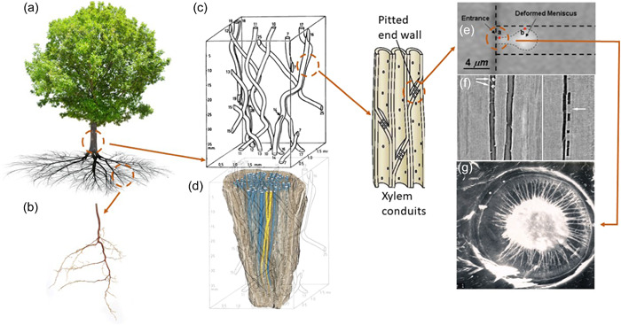
Scales of hydraulic phenomena in woody plants addressed in this review and sections in which each scale is discussed; (a) whole tree scale (1–10 m; Sections 2, 6, and 7); (b) belowground properties of soil–root systems (µm–m; Sections 6 and 7); (c) early work on vessel networks from Zimmerman & Brown (1971) (xylem network scale; µm–m; Sections 4 and 7); (d) more recent work showing vessel network properties, yellow vessels are connected, blue vessels are unconnected, from Johnson et al. (2014); (e) visual observation of air‐seeding in a synthetic nanofluidic channel, from Duan et al. (2012); (f) refilling of an embolized vessel in grapevine, from Brodersen et al. (2018); (g) torus margo pit from Pseudotsuga menziesii, JC Domec, unpublished (panels e, f and g represent bubble and conduit scales; nm–µm; Sections 3, 5 and 7). Although panels (a)–(d) are representative of angiosperms, panel (g) represents the torus margo pits found in some angiosperms (mainly within the Oleaceae, Thymelaeaceae, Cannabaceae and Ulmaceae families; Dute, 2015) and in most conifer xylem which is discussed in Sections 5 and 7 and Box 4. All images are reproduced with permission. [Color figure can be viewed at wileyonlinelibrary.com]

Air molecules (primarily nitrogen) trapped within embryonic bubbles cannot rapidly dissolve by condensation when tension in the xylem drops. To the contrary, water vapour molecules trapped within the bubble can condense almost instantly. Depending on the number of air molecules within an embryonic bubble, these molecules can act to destabilize the bubble with further increases in xylem tension leading to embolism (i.e., blocking of xylem vessels or tracheids by air bubbles), embolism spread, and subsequent hydraulic failure (i.e., loss of overall conductivity of the water delivery network). Embryonic air bubbles of size <1 nm (1 × ${10}^{-9}$ m) can initially grow with increased tension but remain stable and initially harmless.

Beyond a certain bubble size and when in abundance, these air bubbles can push water molecules apart by sufficient distances to weaken the van der Waal attractive forces needed for maintaining cohesion (Szalewicz, 2003). The mean distance between water molecules is 0.3 × ${10}^{-9}$ m (Perkins, 1986) and for simplicity is assumed to be comparable to the ‘equilibrium distance’ where the overall electric potential is minimum. At distances between water molecules far exceeding 0.3 nm, the van der Waal attractive forces decay as an inverse 6th power (instead of inverse square) with increased distance, though it is worth noting that the repulsive forces increase as inverse 12th power for reduced separation distances smaller than 0.3 nm (Israelachvili & Pashley, 1983). Weakening of the attractive forces by the presence of air bubbles can result in loss of cohesion among water molecules. In this situation, the chain defining the water column becomes even more prone to breaking under tension ultimately facilitating overall hydraulic failure.

Frequent or irreparable hydraulic failure sustained over extended periods can result in plant mortality and there are many examples (Adams et al., 2017; Hammond et al., 2019; Rowland et al., 2015; Sevanto et al., 2014). To be clear, the precise pathway by which hydraulic failure causes plant mortality remains a subject of research. Frequent stomatal shut‐down due to elevated xylem tension reduces carbon dioxide uptake by the plant and thus deprives the plant from much needed carbohydrates produced by photosynthesis. Increased xylem tension can also lead to loss of osmotic potential in the phloem thereby preventing delivery of carbohydrates within the plants to where they are needed (Salmon et al., 2019; Sevanto, 2014). Thus, mortality may result from a number of mechanisms such as respiratory costs exceeding photosynthetic gains (Mooney, 1972), weakening of plant defenses (Novick et al., 2012), reducing investment in growth (above or below ground) thereby reducing fitness against neighbouring plants or invasive species (Casper & Jackson, 1997; Manoli et al., 2017), among others. All these mortality considerations begin with elevated tension in the xylem.

Drought induced tree mortality has been observed across the globe (Allen et al., 2010, 2015) and appears to be contributing strongly to loss of resilience in many forests (Boulton et al., 2022). In many studies, the starting point is an assessment of how projected changes in mean air temperatures and precipitation alter the balance between supply and demand for water needed to sustain photosynthesis (Manzoni et al., 2014). Since loss in leaf area is one mechanism by which the plant can reduce its respiratory costs when photosynthetic gains are restricted (Hsiao, 1973), shifts in the variability of leaf area can serve as another tipping point. This latter point was demonstrated from shift in leaf area statistics derived using long‐term satellite records (e.g., Liu et al., 2020). At the cell‐to single plant‐scale, the genesis of the collapse of the plant water transport is amenable to a deterministic treatment, which frames the scope of this review.

Here, a multiscale framework based on catastrophe theory to measure ecological risk of hydraulic failure is proposed. When describing hydraulic failure at multiple scales, we use the word cavitation to indicate the formation of a bubble or cavity in water of finite radius and number of gas molecules. Our definition of an embolism is a cavitation event that leads to air filling of a significant portion of the volume of a single tracheid or a vessel. Thus, embolism is associated with cavitation events where the forces acting on the bubble lead to significant bubble growth. The term embolism spread is used to describe events where air from one embolized vessel or tracheid is spread to an intact and hydraulically connected neighbour resulting in their embolism. We use the term cavitation spread to indicate the transfer of cavities or bubbles from one tracheid or vessel member to an adjacent and hydraulically connected neighbour. Thus, cavitation spread may be preferred to embolism spread in certain cases because it accommodates the possible occurrence of small but harmless embryonic bubbles that can travel from one tracheid or vessel member to another with the water stream without necessarily causing embolism.

The assessment models involve multiple spatial scales that cover the status of bubble formation and expansion, embolism and cavitation spread in xylem and soil, and the hydraulic effects of embolism for plant functioning under changing climate (Figure 1). The results provide guidance for the risk assessment of environment given the strong objectivity of catastrophe theory compared with other evaluation methods. The time is ripe for this undertaking given (i) the proliferation of remote sensing products (NDVI for plants, SMAPS for near‐surface soil moisture and plant water storage, ECOSTRESS for estimating canopy transpiration), (ii) the availability of accessible past, present and projections of large‐scale hydroclimatic variables (e.g., air temperature, water vapour, and precipitation through NCEP reanalysis), and (iii) a wealth of experiments and global public data bases on plant water use (SAPFLUXNET) and hydraulics traits across biomes and species (TRY database and XFT database).

This review will cover scales that span bubbles and cell‐wall mechanics up to whole‐plant as well as environmental controls on them. The work is organized as follows: Section 2 provides an overview of catastrophe theory (equilibrium, stability and bifurcations) at the whole‐plant scale using the von Bartalanffy equation (VBE) for carbon balance. Section 3 revisits these principles using the force‐balance on bubbles within the xylem and establishes the necessary conditions for embolism in a single vessel or tracheid. Section 4 tracks the consequences of embolized vessels and embolism spread on vulnerability curves and reviews a number of hypotheses about their shapes and relations between macroscopic properties characterizing xylem hydraulics (e.g., r‐shaped vs. s‐shaped, Weibull vs. logistic, safety vs. efficiency, and hydraulic segmentation). Section 5 revisits the results in Section 3 with a focus on the role of cell‐wall mechanics in limiting bubble sizes and the shifting of the catastrophe type when describing embolism and its spread. Section 6 explores the below‐ground environment and the controls that soil processes exert on whole‐plant water transport through a balance between soil water supply and plant water demand. Section 7 presents a number of underexplored plant water transport properties and offers suggestions on how to investigate them. Section 8 concludes with a synopsis of the status of the field when viewed from the perspective of catastrophe theory and presents a blueprint for future inquiries.

2. CATASTROPHE AT THE WHOLE‐PLANT SCALE

2.1. What is catastrophe theory?

Hydraulic failure at multiple scales leading to plant mortality shares some resemblance to ‘catastrophe theory’ in dynamical systems (Konrad & Roth‐Nebelsick, 2003; Konrad et al., 2019; Manzoni et al., 2014; Parolari et al., 2014; Thom, 1975; Zeeman, 1976; see also Zeeman, 1978, video). In catastrophe theory, a single differential equation or a set of differential equations represent the temporal evolution of the state variable of the system (e.g., biomass, soil or plant water status, bubble size, etc.). The parameters of these equations needed to describe the temporal trajectory of the state variables are labelled ‘control parameters’. In plant hydraulics, these control variables may be exogenous, such as air molecules that enter a xylem conduit or vapour pressure deficit in the atmosphere, or endogenous, such as xylem tension. Equilibrium points, also known as stagnation points or steady‐state limits, can be derived as a function of these control variables. Gradual variations in these control variables due to a prolonged drought, slow changes in soil nutritional status, gradual increase in elevated atmospheric CO₂, or age‐related factors can lead to sudden shifts in the stability of an existing equilibrium point or appearance and disappearance of equilibrium points. The slow variations in these control parameters are ‘endogenous’ to the dynamical system and differ from ‘exogenous’ disturbances (or shocks) acting on the ecosystem (i.e., ice storm or hurricane diminishing leaf area or plant biomass, forest fires, etc.). When ignoring these exogeneous disturbances and assuming that the control parameters can be treated as predetermined constants to be dialled up or down depending on external conditions, the resulting dynamical system is labelled as ‘autonomous’ and time is no longer an explicit variable.

In their classic book on fluid mechanics, Landau and Lifshitz (1987) state that ‘The flows that occur in Nature must not only obey the equations of fluid dynamics, but also be stable….’. Likewise, ecosystems exist in stable equilibrium states ranging from deserts (i.e., small plant biomass per unit ground area) to tropical forests (plant biomass per unit ground area is large) depending on long‐term rainfall amounts and air temperature (control variables). Catastrophe theory is effective in identifying or delineating ‘tipping points’ in the control variables that alter these equilibrium properties when these control parameters are dialled up or down.

The study of fluid dynamics is full of such examples such as the transition from laminar to turbulent flow, the emergence of convection cells in a heated fluid, or the shape of moving bubbles in fluids due to body forces where the Reynolds, Rayleigh and Bond numbers are the control variables, respectively. In ecosystems, a dramatic case is when a desertification state switches from being an unstable equilibrium point to being a stable equilibrium (Konings et al., 2010). The occurrence of multiple equilibrium points (or alternative stable states) and loss or alteration of their stability is linked to the nature of the non‐linearity governing the dynamics of the system (Strogatz, 1994). It is a topic with long‐standing tradition in the ecological sciences (Hammond, 2020, Scheffer & Carpenter, 2003, Scheffer et al., 2001). Also, in epidemiology, the basic reproduction number (Ro) is a key control parameter deciding whether an emerging infectious disease spreads in a susceptible population (Ro > 1) or not (Hethcote, 2000; Kermack & McKendrick, 1927). In this review, cavitation, cavitation spread, and embolism in the plant xylem share several analogies to infectious disease spread (Roth‑Nebelsick, 2019) and one of the goals of this review is to identify tipping points resembling Ro but for plant hydraulics.

The linkage between equilibrium points (and their stability) and the variations in control parameters as they are increased or decreased is formally studied using ‘bifurcation analysis’ and is the corner stone of catastrophe theory. Bifurcation analysis is illustrated at the individual plant scale using its carbon balance as represented by VBE in what follows.

2.2. The carbon balance of a plant: A dynamical system perspective

The plant carbon balance viewed from the perspective of the VBE considers the processes needed to describe the above ground biomass dynamics. The VBE is given by (Mrad et al., 2020; Perry, 1984; Von Bertalanffy, 1938; see Table 1 for symbol definitions)

$$\frac{\mathit{dB}}{\mathit{dt}}=A_c{P}_{g}L-k_{m}B,$$

where $B$ is above‐ground biomass, t is time, $A_c$ is the proportion of photosynthates allocated to above ground tissue, $P_g$ is the gross photosynthesis per unit leaf area reduced by photorespiration and synthesis respiration, L is the leaf area of the individual plant, and $k_m$ is rate of maintenance respiration plus tissue death. The VBE assumes that a plant harvests resources (photosynthetically active radiation here) through a surface area proportional to L but incurs respirational costs proportional to its biomass (or volume). When naively setting $L=c{B}^n$ (i.e., a presumed allometric relation between size and foliage amount) defined by parameter c and scaling exponent n, the VBE can be expressed as a single‐equation dynamical system given by

$$\dot{B}=\frac{\mathit{dB}}{\mathit{dt}}=f\left(B\right)=\left(A_c{P}_{g}c\right)B^n-k_{m}B=k_{m}B\left(\frac{A_c{P}_{g}c}{k_m}{B}^{n-1}-1\right)=k_{m}B(\alpha B^{n-1}-1),$$

where the overdot indicates differentiation with respect to time as common in the dynamical systems literature (Strogatz, 1994), the parameters $\alpha =A_c{P}_{g}c/k_m,n,$ and $k_m$ are plant‐specific positive constants and $\dot{B}=f\left(B\right)$ is the dynamical system describing the time trajectories of above‐ground biomass from a known initial biomass $B\left(0\right)$ at $t=0$. Von Bertalanffy labelled the constant terms $\left(A_c{P}_{g}c\right)$and $k_m$ as coefficients of anabolism and catabolism, respectively.

Table 1.

Symbols and definitions

A	Area
A c	Proportion of photosynthates allocated to above ground tissue
α	Is equal to: $A_c{P}_{g}c/k_m$
B	Above‐ground biomass
B eq	Above‐ground biomass at equilibrium
b and b’	Control how easily an impaired vessel embolizes a water‐filled one
β	Curvature of the soil water retention curve
c	Median pressure (63rd percentile) necessary for air entry into the biggest pores of the population of pit‐fields or leaf area scaling parameter in VBE
$c_1$	Integration constant in VBE
c a	Atmospheric CO2 concentration
c i	Intercellular CO2 concentration
d	Related to the coefficient of variation of the maximum pore population of pit‐fields
d t	Cell wall thickness
E t	Young's modulus of elasticity
γ	Surface tension coefficient of liquid water
h	Path length from root to leaf
k m	Rate of maintenance respiration plus tissue death
$\kappa$	Coefficient of compressibility for water
K max	Maximum hydraulic conductivity of the xylem
K sat	Saturated soil conductivity
k n	Probability of finding an embolized vessel
K soil, K root, etc.	Hydraulic conductivity of soil, root, etc.
K soil,effective	Effective soil hydraulic conductance characterizing the ease of water flow from the soil pores to a given surface area of root
L	Leaf area
l t	Tracheid length
LAI	Leaf area index
µ	Cell‐wall material compressibility
n	Scaling exponent in VBE
n a	Number of molecules or particles (air, water vapour, and other gases)
n i	Initial number of molecules
n max	Maximum number of molecules
p	Pressure
p*	Saturation vapour pressure
$P_g$	Gross photosynthesis per unit leaf area reduced by photorespiration and synthesis respiration
p s	Xylem pressure
ψ	Xylem tension
ψ l	Leaf tension
ψ o	Reference xylem tension
ψ r	Root water potential
ψ soil	Soil water potential
ψ soil,crit	The soil water potential beyond which soil hydraulics become limiting for water transport in the soil–plant system
ψ xylem	Xylem water potential
ψ 12	Xylem tension (water potential) at 12% loss of conductivity
ψ 50	Xylem tension (water potential) at 50% loss of conductivity
P g	Gross photosynthesis per unit leaf area reduced by photorespiration and synthesis respiration
PLC	Percent loss of conductivity
R	Radius
Ro	Basic reproduction number in epidemiology
RAI	Root area index
RLD	Root length density
R e	Threshold radius for bubble expansion
R m	Maximum bubble radius
r root	Root radius
r soil	Soil radial distance from the roots to the mean distance between roots
r t	Undeformed tracheid radius
$\mathfrak{R}$	Universal gas constant
s crit	Critical degree of saturation
σ t	Poisson number
t	Time
T	Temperature
${\tau }_{\mathrm{eq}}$	Return to equilibrium time scale
T r	Transpiration
$T_{\mathrm{supply}}$	The ability of the soil to supply water to the roots
$\theta$	Contact angle
V	Volume
V(B)	Potential surface in VBE
VBE	von Bertalanffy Equation
VPD	Vapour pressure deficit
W[.]	Principal Lambert W‐function
WUE	Leaf‐scale water use efficiency
x	ψ/ψ o

Returning to the specific trajectory (also known as the particular solution) of the dynamical system $\dot{B}=f\left(B\right)$ in time (see Box 1 and Figure B1 for examples), it depends on the choices made for $\alpha ,n,$ and $k_m$ as well as $B\left(0\right)$. The study of dynamical systems enables the exploration of many properties of the VBE without actually solving this differential equation. By focusing on key points such as the equilibrium or steady‐state points, it becomes possible to assess the long‐term responses of the dynamical systems in relation to the control variables $\alpha ,n$ and $k_m$ without detailed knowledge of the time trajectory from the initial state to the steady‐state.

Box 1: Stability and bifurcation analysis of the von Bertalanffy equation (VBE).

Examples of how the VBE approaches equilibrium states with increasing time are featured in Figure B1. These examples begin with a finite $B\left(0\right)$ and as $t\to \infty$, the steady‐state is approached at a rate and numerical value dictated only by $\alpha$ and n. Equilibrium (or steady‐state) in the VBE is attained upon setting $\dot{B}=0$ and the relation between the control variables $\alpha$ and n and the emergence and stability changes of these equilibrium points is the ‘backbone’ of catastrophe theory. There are only two equilibrium states for the VBE: $B_{\mathrm{eq},1}=0$ (i.e., death or extinction) and $B_{\mathrm{eq},2}={\alpha }^{1/(1-n)}$ (finite biomass). These two equilibrium points may be either stable or unstable depending on the numerical value of $\alpha$ and n. The case where L scales linearly with aboveground biomass ($n=1$) leads to loss of all non‐linearities and only one equilibrium point exists: $B_{\mathrm{eq},1}=0$. For $\alpha >1$, this equilibrium point is unstable and B grows exponentially as $t\to \infty$. For $\alpha <1$, this equilibrium point is stable and is asymptotically approached as $t\to \infty$. Thus, the dynamically interesting case is when $n\ne 1$ where the stability of the two equilibrium points $B_{\mathrm{eq},1}=0$ and $B_{\mathrm{eq},2}={\alpha }^{1/(1-n)}$ can be assessed using linear analysis. In linear analysis, a small biomass perturbation $\delta B$ to the equilibrium state ($B_{\mathrm{eq}}$) is introduced and its growth or decay in time is then analyzed. Setting $B=B_{\mathrm{eq}}+\delta B$ and recalling that $\dot{B}=f\left(B\right)$, the dynamical system can be expressed as

$$\dot{B_{\mathrm{eq}}}+\dot{\delta B}=f(B_{\mathrm{eq}}+\delta B)=f\left(B_{\mathrm{eq}}\right)+{\left.\frac{d}{\mathit{dB}}f\left(B\right)\right|}_{B_{\mathrm{eq}}}\delta B+H.O.T,$$

where H.O.T. stands for higher‐order terms of the Taylor series expansion applied to $f(B_{\mathrm{eq}}+\delta B)$ around the aforementioned two $B_{\mathrm{eq}}$ values. At equilibrium, $\dot{B_{\mathrm{eq}}}=f\left(B_{\mathrm{eq}}\right)=0$ resulting in

$$\dot{\delta B}={\left.\frac{d}{\mathit{dB}}f\left(B\right)\right|}_{B_{\mathrm{eq}}}\delta B=f^{\prime }\left(B_{\mathit{e}\mathit{q}}\right)\delta B,$$

where primed quantities indicate differentiation with respect to the state variable B instead of time. Hence, the temporal evolution of the biomass perturbation around the $B_{\mathrm{eq}}$ is governed by

$$\frac{\delta \dot{B}}{\delta B}=f^{\prime }\left(B_{\mathrm{eq}}\right).$$

Provided $f^{\prime }\left(B_{\mathrm{eq}}\right)\ne 0$, $\delta B$ can grow exponentially in time away from $B_{\mathrm{eq}}$when $f^{\prime }\left(B_{\mathrm{eq}}\right)>0$ (i.e., $B_{\mathrm{eq}}$ is an unstable equilibrium) or decays exponentially in time back to $B_{\mathrm{eq}}$ when $f^{\prime }\left(B_{\mathrm{eq}}\right)<0$ (i.e., $B_{\mathrm{eq}}$ is a stable equilibrium). The discussion above applies to any first‐order dynamical system expressed as $\dot{B}=f(B).$

For the specific $\dot{B}=f\left(B\right)$ given by the VBE,

$$f^{\prime }\left(B_{\mathrm{eq}}\right)=k_m\left(n\alpha {B_{\mathrm{eq}}}^{n-1}\mathrm{–}1\right).$$

In the case of $B_{\mathit{eq},2}={\alpha }^{1/(1-n)},$

$$f\prime \left(B_{\mathrm{eq},2}\right)=k_m\left(n\mathrm{–}1\right).$$

Interestingly, the stability of $B_{\mathrm{eq},2}$ only depends on the degree of non‐linearity n set by the allometric relation between size B and foliage amount L. For $n>1$, $B_{\mathrm{eq},2}$ is unstable whereas for $n<1$, this equilibrium biomass is stable. For many species, the reported $n=0.46-0.88$ (mean of $n=0.84$) with the lower range of $n$ associated with species that are highly intolerant to shade and conversely (Perry, 1984). This range is consistent with the stability requirement that $n<1$ for a non‐extinction equilibrium to exist (i.e., $B_{\mathrm{eq},2}={\alpha }^{1/(1-n)}$).

Returning to the stability of $B_{\mathrm{eq},1}\to 0^{+}$ (i.e., death or extinction) approached from a positive biomass end,

$$f\prime \left(B_{\mathrm{eq},1}\right)=k_m\left[n\alpha {\left(0^{+}\right)}^{n-1}\mathrm{–}1\right].$$

For $n<1$, $B_{\mathrm{eq},1}=0$ is unstable (i.e., $f^{\prime }(B_{\mathit{eq},1})>0$) whereas for $n>1$, $B_{\mathrm{eq},1}=0$ is stable (i.e., $f^{\prime }\left(B_{\mathrm{eq},1}\right)<0$). When ${B>B}_{\mathrm{eq},2}$ and $n>1$, the dynamical system does not go back to $B_{\mathrm{eq},2}$ but exhibits a so‐called ‘finite‐time’ singularity—meaning that biomass blows up ($\mathrm{i}\text{.}\mathrm{e}\text{.,} B\to \infty$) in a finite amount of time. In this case, the VBE reduces to the much‐studied ‘doomsday’ equation (Kaack & Katul, 2013; Parolari et al., 2015; Sornette, 2002).

In catastrophe theory, the visualization of the stability of equilibrium points is aided when they are placed on a so‐called ‘potential surface’ (Strogatz, 1994; Zeeman, 1976). This surface is specified by a function $V\left(B\right)$ and is mathematically given as

$$\dot{B}=f(B)=-\frac{\mathit{dV}}{\mathit{dB}}=-V^{\prime }(B).$$

The term ‘potential’ originates from the fact that $B$ represents a biomass position (on the real line), $\dot{B}$ is thus analogous to a change in position with respect to time or a velocity, and $f(B)$ may be viewed as analogous to an external force that is balanced by linear friction per unit mass (i.e., $\dot{B}$) when viewed from the force balance $\dot{B}=f(B)$. Taking this analogy one step further, $\mathit{dV}=-f(B)\mathit{dB}$ becomes analogous to incremental work defined by the product of the aforementioned external force $f(B)$ acting on the system and the incremental distance $\mathit{dB}$ on the real line. The negative sign in $\mathit{dV}=-f(B)\mathit{dB}$ is needed to ensure that

$$\dot{V}=\frac{\mathit{dV}}{\mathit{dt}}=\frac{\mathit{dV}}{\mathit{dB}}\frac{\mathit{dB}}{\mathit{dt}}=-f(B)\frac{\mathit{dB}}{\mathit{dt}}=-{(\dot{B})}^2.$$

Hence, $\dot{V}$ always decreases with increasing time until reaching $\dot{B}=0$ (i.e., equilibrium point) via a trajectory that always follows a path of decreasing potential.

For the VBE,

$$V(B)=-\int f(B)\mathit{dB}=\frac{1}{2}{k}_m{B}^2\left(1-\frac{2\alpha }{1+n}{B}^{n-1}\right)+C_1,$$

where $C_1$ is an integration constant that can be set to zero (or any arbitrary number). The potential surface for $n=0.84$ (mean value across many species) and $n=1.2$ while maintaining $\alpha =0.95$ the same are shown in the Figure B1. The $B_{\mathit{eq},2}$ is a stable equilibrium for $n=0.84$ (as expected) whereas extinction or death is unstable as evidenced by the curvature of $V(B)$. For $n=1.2$ the curvatures shift and the $B_{\mathrm{eq},2}$ is no longer stable whereas extinction now is. This shift in stability of the two equilibrium points as $n$ transitions from sub‐unity to super‐unity is a hallmark of what is known as ‘transcritical bifurcation’ where stability points do not appear or disappear. They only alter their stability with respect to the control variable (here $n$) as $n=1$ is crossed. Thus, the VBE illustration makes the link between bifurcation type (transcritical) and the degree of non‐linearity n characterizing the dynamical system explicit.

The curvature of the potential surface in Figure B1 can also be used to assess resiliency or its loss when the control parameter (e.g., n) is gradually changing. When the curvature is small (deep potential well), resiliency is high. Conversely, when the curvature is large (a shallow potential well), resiliency is small and this may be used to signify an approach to a critical state (or a tipping point). More common is the use of a characteristic time (${\tau }_{\mathrm{eq}}$) to return to equilibrium after introducing a perturbation to the system state (e.g., $\delta B$). Return to equilibrium time may be determined from the dynamical system using an e‐folding estimate

$$\left|\frac{\delta \dot{B}}{\delta B}\right|=\left|f^{\prime }\left(B_{\mathrm{eq}}\right)\right|=\frac{1}{{\tau }_{\mathrm{eq}}}.$$

In the VBE analyzed here, this return to equilibrium time for the finite biomass equilibrium case (i.e., $B_{\mathrm{eq},2}$) is given by

$${\tau }_{\mathrm{eq}}=\left|\frac{1}{k_m\left(n\mathrm{–}1\right)}\right|={\left|\frac{d^{2}V}{d{B}^2}\right|}_{B_{\mathrm{eq},2}}^{-1}.$$

The above result shows how ${\tau }_{\mathrm{eq}}$ is related to the curvature of $V(B)$ at the equilibrium point $B_{\mathrm{eq},2}$. As $n\to 1$, ${\tau }_{\mathrm{eq}}$ becomes very large and the curvature of $V(B)$ becomes flat, a phenomenon labelled as ‘critical slowing down’.

In ‘noisy’ but long time series of biomass, it is possible to fit a first‐order autoregressive or AR(1) process to a smaller time window using standard methods (Liu et al., 2019). A ${\tau }_{\mathrm{eq}}$ can then be computed from the autocorrelation function of the AR(1) process for that window. As the window is moved forward in time across the noisy biomass record, an assessment of whether ${\tau }_{\mathrm{eq}}$ is increasing (signifying loss or resilience) or not can then be made. There is a unique relation between the parameter of an AR(1) process, its autocorrelation function, and ${\tau }_{\mathrm{eq}}$ and often this parameter is featured instead of ${\tau }_{\mathrm{eq}}$. The aforementioned tactic of fitting AR(1) to noisy data and inferring ${\tau }_{\mathrm{eq}}$ has been effective at delineating loss of resiliency from satellite‐based remotely sensed forest biomass data at large spatial scales as discussed elsewhere (Boulton et al., 2022; Liu et al., 2019; Wu et al., 2022).

Figure B1.

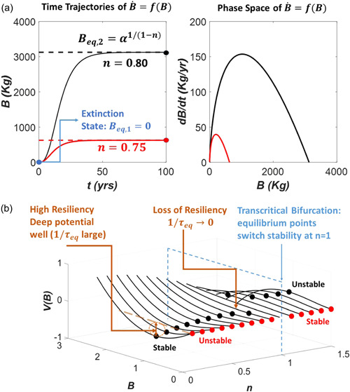
(a) Illustration of the trajectories (left) and the phase‐space (right) for the VBE dynamical system for two control parameters: n = 0.75 and n = 0.80. The remaining parameters ($k_m$ = 0.6 per year, $\alpha$ = 5, and $B\left(0\right)$ = 0.1 kg) are the same for both cases. The two equilibrium points are also shown corresponding to $\mathit{dB}/\mathit{dt}=0$. The bifurcation analysis is conducted on the equilibrium biomass with the allometric scaling exponent n being the control parameter shown later in panel b. (b) The variations of the potential surface $V(B)$with B and n for $\alpha =0.95$. The two equilibrium points $B_{\mathrm{eq},2}={\alpha }^{1/(1-n)}$ and $B_{\mathrm{eq},1}=0$ are shown as black and red circles, respectively. Based on the convexity of V(B), the equilibrium state for $B_{\mathrm{eq},1}$ and $B_{\mathrm{eq},2}$ can be determined. For $n<1,B_{\mathrm{eq},2}$ is stable whereas $B_{\mathrm{eq},1}=0$ is unstable. For $n>1$, the stability of these equilibrium points reverses. Thus, a ‘catastrophe’ occurs when $n$ transitions from subunity to super‐unity (i.e., transcending or crossing a critical state). This bifurcation on the control parameter $n$ is known as ‘trans‐critical’ because no new equilibrium points are produced (or lost)—only their stability is exchanged with $n$ crossing a critical value of unity. This catastrophe is termed as ‘fold’ (Zeeman, 1976). The resiliency of this system is high because there is only one stable equilibrium point (instead of multiple stable equilibria). However, starting from $0<n<1$ and as the critical n = 1 is approached, the potential surface at $B_{\mathrm{eq},2}$ becomes shallower and shallower. At n = 1, the potential surface becomes entirely flat resulting in a collision between the two equilibrium points followed by a shift in their stability. That the potential is becoming shallower as the critical exponent n is approached is a signature of loss of resiliency—and can be used as an early warning signal of an impending catastrophe (in this case, a zero above ground biomass, i.e., plant death). [Color figure can be viewed at wileyonlinelibrary.com]

Before exploring these key points, a clarification about the use of the term equilibrium versus steady state is in order. These terms are used interchangeably in dynamical systems theory when expressed as $\dot{B}=f\left(B\right)$. However, in thermodynamics, clarifying this difference is fundamental. Thermodynamic and dynamical systems considerations are both employed later on in Section 3, which is why this informal digression is undertaken here. Thermal equilibrium, for example, implies that the temperature between two objects that are in contact and can exchange energy be the same. Steady state implies that the temperature of the object or objects in contact with each other be constant with respect to time. Likewise for the remaining two types of equilibria in thermodynamics: mechanical (dealing with volume expansion and contraction) and chemical (dealing with movement and amounts of particles). Hence, a system can be in steady state but not in thermal equilibrium. A rod being heated at one end and losing the same amount of heat per unit time at the other end may be in steady state after long times but not in thermal equilibrium. Last, a system interacting with its environment may attain one type of thermodynamic equilibrium but this attainment does not imply equilibrium for the other two types. For instance, a hot air balloon interacts thermally, mechanically and diffusively with the surrounding atmosphere at certain times—but not all these interactions are at equilibrium at all times.

Returning to the response of a plant to an extended drought, this response occurs at multiple time scales (Hsiao, 1973) that can be partly accommodated by the VBE. On physiological time scales (i.e., time scales commensurate with stomatal opening and closure), droughts reduce the hydraulic capacity of the xylem to deliver water so as to sustain the biochemical demand for carbon dioxide thereby reducing the value of $P_g$. On intermediate time scales (i.e., allocation of carbon), $A_c$ is reduced so as to allocate more carbon to belowground tissue construction needed for enhancing access to water and nutrients in the soil. On even longer time scales, foliage shedding occurs reducing L and altering the allometry linking L to B by adjusting $c$ and/or n. Likewise, $\alpha$ and n can vary with elevated atmospheric CO₂ or nutritional status of the soil.

When these parameters vary slowly in time (e.g., due to climate change), then they can be treated as control variables in the VBE thereby making this dynamical system autonomous and amenable to bifurcation analysis. The latter is necessary for identifying tipping points deterministically as a function of the control variables as illustrated in Box 1. The equilibrium (or steady‐state) points for the VBE here are $B_{\mathrm{eq},1}=0$ (i.e., death or extinction) and $B_{\mathrm{eq},2}={\alpha }^{1/(1-n)}$ (finite biomass). Box 1 illustrates how the stability of these two equilibrium biomass values changes when the exponent $n$ (control variable) gradually increases and crosses unity (critical value). In particular, Box 1 establishes links between the bifurcation type (known as transcritical here because a critical value $n=1$ is crossed with increasing $n$) and the degree of non‐linearity (i.e., $n$) characterizing the dynamical system. Many of the phenomena in the plant world, from patterns of tree mortality (Boulton et al., 2022, Dietze & Moorcroft, 2011) to xylem loss of hydraulic conductivity (Sperry et al., 1994) and spruce budworm outbreak (Ludwig et al., 1978) are non‐linear in nature and often display similarities to the catastrophe. In fact, there are striking similarities between the spruce budworm outbreak and occurrence of embolism in xylem vessels when cell‐wall mechanics is included to be illustrated later on in Section 5.

2.3. Hydraulic failure and catastrophes: From bubble to whole‐plant

The connection between catastrophe theory and hydraulic failure in plants has been receiving some attention in various forms and across scales spanning single bubble, whole plants and forests. The work here aims to show similarities in the catastrophe across scales, highlight the control variables, and expand upon the processes needed to describe the control variables and the mechanisms they espouse to represent. To illustrate catastrophe theory at all these scales, the approaches in Konrad and Roth‐Nebelsick (2003) and Manzoni et al. (2014) are used.

3. BUBBLE SCALE

The connections between catastrophe theory and hydraulic failure at the bubble scale commences with an isolated spherical bubble of initial radius R that appears in a xylem conduit. The focus is not on how a collection of ‘pioneering’ air molecules entered a particular xylem conduit but whether the initial bubble radius will expand or contract depending on the expanding versus contracting forces acting on the bubble. If the ‘pioneering’ air molecules result in bubble radii that are unstable, the bubble may expand or even explode (and release acoustic energy; e.g., Millburn & Johnson, 1966). The infected conduit fills up rapidly with air (and water vapour) and becomes hydraulically dysfunctional or embolized. If the adjacent conduit is hydraulically functional, the air molecules can then spread from the dysfunctional to the functional conduit depending on the membrane properties separating the two conduits and their state (to be considered in Section 5). The ease of spread of air molecules from dysfunctional to functional conduits in this manner is the essence of the so‐called air‐seeding hypothesis (Zimmermann, 1983).

Returning to the pioneering air molecules infecting an isolated conduit, the stability of the bubble radius from its initial or embryonic state forms the basis of a dynamical system that is shown to exhibit a (fold) catastrophe when the three key control parameters are slowly varied. These control variables are background liquid xylem pressure $p_s$ (i.e., negative or positive for now), initial R (bubble radius), and the amount of molecules or particle number $n_a$ (including nitrogen, water vapour and other gases) trapped inside the bubble. The bubble is assumed to be spherical with initial volume $V=(4/3)\pi R^3$ and initial surface area $A=4\pi R^2.$ The Bond number of the bubble is assumed to be very small so that gravitational forces can be neglected relative to surface tension.

Throughout, it is assumed that the bubble and the liquid water in the xylem are in thermal equilibrium so that the temperature T is the same throughout and no heat exchange occurs.

Mechanical equilibrium requires that the gas pressure inside the bubble $p$ (produced by random collisions between gas molecules within the bubble and the bubble interface) acting in an outward‐directed force be balanced by the net pressure at the bubble interface. The absence of a mechanical equilibrium leads to rapid changes in bubble radius (contraction or expansion). Representing the transient phases of these changes necessitates the inclusion of viscous forces, local and advective acceleration terms resulting in the Rayleigh‐Plesset equation (see Hölttä et al., 2007; Plesset & Prosperetti, 1977). However, at equilibrium, $p$ in the bubble is balanced by surface tension ($2\gamma /R$, where $\gamma =$ 72 mN m⁻¹ at standard temperature is the surface tension coefficient of liquid water expressed in force per unit length) that acts to contract the bubble and background xylem liquid pressure $p_s$ that acts to expand (when in tension) or contract (when in compression) the bubble. Thus, the force balance along the bubble surface leads to

$$p=p_s+\frac{2\gamma }{R},$$

which is the Young–Laplace equation. When $p>p_s+\frac{2\gamma }{R}$, the bubble grows whereas when $p<p_s+\frac{2\gamma }{R},$ the bubble contracts. At equilibrium, p is higher than p _s of the surrounding liquid. To illustrate typical bubble sizes, consider a bubble pressure that is close to atmospheric (= +0.1 MPa) and $p_s=-2$ MPa (typical operating xylem pressure in many tree species), equilibrium leads to bubble sizes that are on the order of

$$R=\frac{2\gamma }{p-p_s}=0.06 \mathrm{\mu m},$$

or some 230 times the mean distance between water molecules. In general, the pressure $p$ inside the bubble depends on $n_a$ and T when not atmospheric. To proceed further, it is assumed that the gas in the bubble is ideal so that (Konrad & Roth‐Nebelsick, 2003)

$$n_a\left(R\right)=\frac{\mathit{pV}}{\mathfrak{R}T}=\frac{4\pi }{3\mathfrak{R}T}{R}^3\left(p_s+\frac{2\gamma }{R}\right)=\frac{4\pi }{3\mathfrak{R}T}(p_s{R}^3+2\gamma R^2),$$

where $\mathfrak{R}=8.314$ m³ Pa mol⁻¹ K⁻¹ is the universal gas constant. This expression has an equilibrium point at R = 0 (irrespective of $p_s$) where $n_a\left(R\right)=0$ and the embryonic bubble is assumed to have dissolved in the xylem (i.e., safe). Stability of the bubble can now be assessed based on the initial number of particles $n_i$ trapped in the bubble at some initial radius R when referenced to the maximum allowed $n_a\left(R\right)$ determined at equilibrium from the combination of the ideal gas law (at constant T) and the Young–Laplace equation.

When $p_s>0$ (as may be expected at night when the soil is near saturation), $n_a\left(R\right)$ is a monotonically increasing function of R as shown in Figure 2. Thus, when $n_i$ differs from $n_a\left(R\right)$, the bubble will expand (when $n_i>n_a\left(R\right)$) or contract (when $n_i<n_a\left(R\right)$) until the equilibrium point $n_i=n_a\left(R\right)$ is reached. However, this equilibrium point remains a stable equilibrium point and the radius of the bubble adjusts until $n_i=n_a\left(R\right)$ at this equilibrium. There is a single stable equilibrium radius associated with this positive xylem pressure state and thus no catastrophe exists.

Figure 2.

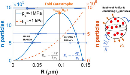
Analysis of bubble stability represented by the number of initial molecules (n_i ) as a function of bubble radius ( R ) that can be accommodated under two xylem pressures (p_s ) using the formulation in Konrad and Roth–Nebelsick (2003). When ${n_i<n}_{\max }$ and ${R<R}_{\mathrm{e}}$, the bubble remains stable and harmless to the xylem (i.e., the initial bubble will grow or shrink to the stable branch). When ${n_i<n}_{\max }$ and ${R>R}_{\mathrm{e}}$, the bubble will grow and may burst. When ${n_i>n}_{\max }$, the bubble will rapidly grow and may burst. When p_s  > 0, there is no catastrophe and a single stable equilibrium exist (dashed line). When p_s  < 0, the catastrophe is of a ‘fold’ type with one stable (or attractive) branch and one repelling (or unstable) branch. The saddle point defining the fold catastrophe is the point (R _m , n _max). [Color figure can be viewed at wileyonlinelibrary.com]

When $p_s<0$ (typical of xylem pressures during the day when transpiration or water stress occurs), the situation is different. To begin with, a new state is created as $p_s$ changes from positive to negative. This new state can be determined when $n_a\left(R\right)$ = 0 and requires $p_s{R}^3+2\gamma R^2=0;R_e=-2\gamma /p_s>0.$ This is the maximum possible radius that can be reached by the bubble under tension $p_s$ without bubble bursting (Konrad & Roth‐Nebelsick, 2003).

The maximum number of molecules $n_{\max }$ that can be accommodated at any $p_s<0$ can also be computed by setting

$$\frac{d{n}_a\left(R\right)}{\mathit{dR}}=\frac{4\pi }{3\mathfrak{R}T}({3p}_s{R}^2+4\gamma R)=0,$$

solving for the radius

$$R_m=\frac{-4\gamma }{{3p}_s},$$

and inserting this estimate of the radius into the $n_a\left(R\right)$ yields (Konrad & Roth‐Nebelsick, 2003)

$$n_{\max }\left(R_m\right)=\frac{2\pi \gamma }{\mathfrak{R}T}{\left(\frac{8\gamma }{9p_s}\right)}^2.$$

The radii $R_m$ and $R_e$ and associated $n_a\left(R\right)$ at equilibrium are shown in Figure 2. Three cases are considered:

When ${n_i>n}_{\max }$, the bubble expands and embolism occurs.

When ${n_i<n}_{\max }$ and ${R<R}_e$, the bubble remains stable (and harmless to the xylem).

When ${n_i<n}_{\max }$ and ${R>R}_e$, the bubble expands and embolism occurs.

These three regimes are similar to those derived from thermodynamic considerations discussed elsewhere (Konrad & Roth‐Nebelsick, 2005; Shen et al., 2012). As shown in Figure 2, the point $n_{\max }\left(R_m\right)$ represents a saddle node formed by the intersection of the stable and unstable branches of the equilibrium $n_a\left(R\right)$ curve (Figure 2). The catastrophe associated with this saddle node is typical of a fold catastrophe (Zeeman, 1976). As seen later on, the inclusion of cell‐wall mechanics restricts the size the bubble can expand into thereby adding another equilibrium point and switching the catastrophe from fold to cusp (discussed in Section 5).

The analysis thus far did not distinguish between vapour and air molecules in $n_a$ as their summed partial pressures defines the total gas pressure in the bubble. When a bubble bursts, vapour molecules can instantly condense onto any remaining liquid water in the tracheid or vessel but the solubility of air molecules in water is quite low. Hence, it may be beneficial to track the initial gas composition of the molecules occupying the bubble. To do so, a number of simplifications are made.

Consider an embryonic bubble composed of air molecules only with no vapour molecules ($n_a$ does not include any vapour). When an embryonic bubble forms, liquid water molecules in contact with the bubble surface vaporize instantly into the bubble and thus lead to an increase in the number of gas molecules within the bubble. To estimate the order of magnitude correction to the total pressure when separately treating contributions from vapour pressure arising from instant vaporization and the initial air partial pressure, thermal equilibrium is assumed and no energy exchange is accounted for between the bubble and its liquid surrounding. Moreover, it is assumed that any diffusion of air molecules from the bubble into the liquid can be momentarily ignored given the low solubility of air in water and the fast time scale of evaporation. Thus, to a leading order, water vapour molecules will continue to fill the bubble until the saturation vapour pressure ($p^{*})$ is reached inside the bubble.

Because saturation vapour pressure is only dependent on T, and the analysis thus far assumes thermal equilibrium, $p^{*}$ can be approximated from the Clausius–Clayperon equation. This pressure is, for all practical purposes, contributing to the expansion force of the bubble. Hence, the presence of water vapour molecules may be accommodated by replacing $p_s$ with $p_s-p^{*}.$ In the case when $p_s$ is negative (tension), inclusion of water vapour molecules increases the apparent tension by an extra $p^{*}$ that surface tension has to now resist. Roughly, for T = 20°C, the Clausius–Clayperon equation estimates $p^{*}\approx 2.5 \text{kPa}$ but typical $p_s$ in the xylem during droughts is on the order of −1 MPa. Hence, the role of water vapour molecules can be ignored at xylem tensions exceeding 0.1 MPa though it can be included for completeness in any stability analysis by replacing $p_s$ with $p_s-p^{*}.$ Thermal equilibrium is unlikely during such phase transition (i.e., energy is exchanged) and air inside the bubble may differ from saturation depending on differences in chemical potential between the water surface and the bubble. These refinements can also be included in estimates of $p^{*}$ though they are unlikely to alter the order of magnitude analysis (meaning $\text{kPa}$ for $p^{*}$ vs. MPa for xylem tension).

Last, bubbles that make contact with flat vessel walls (when $p_s<0$) require energy to detach and experience weakening of the restoring force due to finite contact angles (i.e., $\gamma$ becomes $\gamma \cos \mathrm{}\left(\theta \right)$ where $\theta$ is the contact angle). In the case of non‐flat wall vessels, other factors may become significant and can mitigate some of the energy needed for detachment (Konrad & Roth‐Nebelsick, 2009).

There are a number of counteracting effects that play a role in mitigating the effect of unstable bubble growth. With rapid bubble expansion, an expanding bubble may isolate some water in the embolized vessel from the intact vessel. Due to its incompressibility, the trapped water in the embolized vessel begins to experience a reduction in tension or even a local positive pressure (in contrast to the negative pressures within the functioning conduits) thereby promoting a faster dissolution of the gas bubble (Konrad & Roth‐Nebelsick, 2003). This ameliorating effect appears to be supported by other arguments based on geometric considerations of bordered pit structure during refilling discussed elsewhere (Holbrook & Zwieniecki, 1999; Zwieniecki & Holbrook, 2000).

4. MOVING FROM BUBBLE TO XYLEM NETWORK HYDRAULICS

The previous analysis considered the ‘catastrophe’ of an isolated bubble using two control variables: the background liquid pressure in a xylem conduit and initial number of air molecules in an isolated bubble. The necessary conditions for a bubble to become ‘unstable’ from its initial state were established using these two control variables. Unstable bubbles ‘fill' a large portion of the vessel member with air but the ‘ease’ over which air can be transmitted from an embolized vessel member to another functional vessel remains a topic of active research. The current hypothesis is, as noted earlier, ‘air seeding’ (Zimmermann, 1983), where the water tension in the functional vessel is sufficiently large to overcome the membrane (or collection of pit‐fields) separating the two vessels and thus ‘suck’ air molecules from the cavitated vessel into the intact vessel (Figure 1e).

The ease of air seeding and subsequent embolism spread is encoded in the xylem vulnerability curve (Figure 3). Vulnerability of xylem to embolism is thus expressed by curves that depict the accumulating loss of hydraulic conductivity (or the percentage loss of conductivity exhibited) relative to the minimum $p_s$ experienced by the organ (e.g., leaf, branch, stem or root). Without theoretical vulnerability curves, most plant‐scale hydraulic models use empirical formulations (Sperry & Tyree, 1988) with the exponential‐sigmoid function being the most popular due to its simplicity and to its analytical tractability allowing statistical comparisons of its coefficients (Pammenter & Vander Willigen, 1998).

Figure 3.

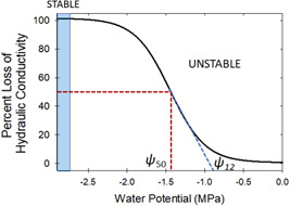
A typical xylem vulnerability curve (VC) as a function of xylem tension (water potential). When xylem tension is increasing with increasing time, the percent loss of conductivity (PLC) = 0% is an ‘unstable equilibrium’ whereas infinite xylem tension leads to a stable equilibrium at PLC = 100%. The ψ ₅₀ and ψ ₁₂ are the xylem tensions at 50% and 12% loss of conductivity, respectively. Derivation of ψ ₁₂ follows Domec and Gartner (2001). At least one vessel member must be embolized to initiate small deviations from the zero‐water potential state. [Color figure can be viewed at wileyonlinelibrary.com]

The vulnerability curve fit to data allows determining coefficients that have a physiological significance and that can be compared among species and plant parts such as, ${\psi }_{50}$, which represents the xylem pressure causing 50% loss of the initial hydraulic conductivity (Ogle et al., 2009). In addition, the end of the initial flat zone of those sigmoidal vulnerability curves can be interpreted as ‘air entry point’ and represents the xylem pressure causing 12% loss of the initial hydraulic conductivity (${\psi }_{12}$; Domec & Gartner, 2001; Meinzer et al., 2009). The extension of the initial flat zone and the steepness of the vulnerability curves depends on interconnectivity and pit membrane resistance to cavitation as derived from the Young–Laplace equation (Mrad et al., 2021; Roth‐Nebelsick, 2019).

Those fitted empirical curves are needed to characterize vulnerability to embolism of a given sample by deriving xylem pressure benchmarks, but from a theoretical point of view the vulnerability of a xylem network can be described from the occurrence of unstable bubbles in tracheids or vessel members. Thus, in a network of inter‐connected vessels, it is convenient to classify these vessels in a binary manner: embolized (and hence hydraulically dysfunctional) and intact (and hence able to transmit water at maximum hydraulic capacity).

In the derivation of vulnerability curves, the overall xylem tension (or air pressure) is increased gradually in time. As the xylem tension is increased, it is convenient to define the probability of finding an embolized vessel as $k_n$ (hydraulically non‐functional) and thus the probability of finding an intact vessel is ${1-k}_n$. For embolism to spread in this idealized network due to gradual increases in xylem tension or air pressure with time, it is necessary for an embolized vessel to be adjacent to a water‐filled one (Meyra et al., 2011). In its most elementary form, this argument leads to a ‘self‐limiting’ embolism spread when xylem tension is incrementally increased as follows:

$$\frac{d{k}_n}{\mathit{dx}}=b{k}_n(1-k_n),$$

where $x=\psi /{\psi }_o$ is a normalized xylem tension referenced to some xylem tension ${\psi }_o$ (to be specified later), $\psi$ is the overall xylem tension, $k_n(1-k_n)$ represent the interaction between a dysfunctional and intact vessel, and $b$ measures how easily an impaired vessel embolizes a water‐filled one. By interaction here, we are referring to the probability that an embolized vessel finds (or makes contact with) an adjacent intact vessel with $b$ reflecting the infection or spread potential of unstable bubbles from the embolized to the intact vessel. Thus, $b$ encodes all the network information about pit‐membranes and the network connectivity among vessel members (this coefficient was set to unity in the work of Meyra et al., 2011). This equation describing the vulnerability of the xylem network with increased air pressure due to the occurrence of unstable bubbles has two equilibrium points: $k_n=0$ (no embolism) and $1-k_n=0$ (completely dysfunctional hydraulically). Stability analysis shows that $k_n=0$ (no embolism) is an unstable equilibrium whereas $k_n=1$ is a stable equilibrium at infinite times or infinite xylem tension.

The solution of this differential equation when $b$ is a constant yields a logistic vulnerability curve or percent loss of conductance (PLC) for $x$ > 0 given by

$$\mathit{PLC}=k_n=1-\frac{1}{1+\mathit{exp}[\mathit{bx}-c_1]},$$

where $c_1$ is an integration constant. Clearly, this solution does not result in a $k_n=0$ when $x=0$ because the exponential term is always positive in the derived PLC expression. This is consistent with the fact that one xylem conduit must be ‘infected’ with air molecules and experience unstable bubble growth before air seeding can be initiated in the entire xylem network (i.e., $k_n>0$ for $x\ge 0$). It is possible to mathematically enforce the conditions that at $x=1$, $k_n=1/2$ so that ${\psi }_o={\psi }_{50}$ (as is conventional in plant hydraulic experiments) and that asymptotically $k_n\to 0$ for $x\to 0^{+}$ (i.e., approached from the positive tension side), the vulnerability curve can now be expressed as a single parameter curve

$$\mathit{PLC}\left(x\right)=\frac{1}{1+\frac{\text{exp}(b)-1}{\text{exp}(\mathit{bx})-1}},$$

where embolism spreads by air seeding (encoded by b) though at least one xylem conduit must have experienced unstable bubble growth and hydraulic impairment. In fact, embolism spread in the xylem and disease spread within a susceptible population share many similarities and have been used to explain rich varieties of PLC(x) shapes (Roth‑Nebelsick, 2019) further discussed in Box 2. Figure 4 shows the measured and modelled PLC(x) across three species ranging from desert shrubs to riparian trees. This figure is suggestive that the derived PLC(x) is sufficiently generic to capture many essential elements of cavitation spread through ${\psi }_{50}$ and b.

Box 2: Stability analysis, r‐shaped and s‐shaped vulnerability curves.

Stability analysis: When xylem tension increases with increasing time (i.e., $\mathit{dx}/\mathit{dt}>0$), the spread of embolism is given by the dynamical system

$$\frac{d{k}_n}{\mathit{dx}}=\frac{d{k}_n}{\mathit{dt}}\frac{\mathit{dt}}{\mathit{dx}}={\mathit{bk}}_n(1-k_n)=f(k_n).$$

In this version, it is assumed that $x$ gradually increases with increasing time and equilibrium states can be interpreted as the states corresponding to either $t\to \infty$ or $x\to \infty$. As expected, only two equilibrium states emerge here and can be determined from ${\mathit{dk}}_n/\mathit{dt}=0$ or ${\mathit{dk}}_n/\mathit{dx}=0$. These states are $k_n=0$ (no dysfunctional conduits) and $(1-k_n)=0$ or $k_n=1$ (all conduits are dysfunctional). As discussed in Box 1, the stability of these two equilibrium points can be assessed by evaluating $f^{\prime }(k_n)=df(k_n)/{\mathit{dk}}_n=b^{\prime }(1-2k_n)$.

At $k_n=0$, $f^{\prime }(k_n)=b^{\prime }>0$ (unstable) whereas at $k_n=1$, $f^{\prime }(k_n)={-b}^{\prime }<0$ (stable). Hence, when introducing bubbles into the xylem conduit and increasing tension indefinitely, the fate of this network at equilibrium is a network where all conduits are dysfunctional.

r‐shaped and s‐shaped vulnerability curves: Vulnerability curves can be described as having two general shapes: (1) an s, or sigmoid shape, and (2) an r, or exponential rise to a maximum (plateau) value. There has been much debate over whether r‐shaped curves are due to measurement artefacts when producing vulnerability curves (Cochard et al., 2010; Martin‐StPaul et al., 2014). However, others have argued that many r‐shaped vulnerability curves are not products of artefacts (Sperry et al., 2012). Additionally, some have argued for fitting logistic models to vulnerability curves whereas others have suggested Weibull functions (Ogle et al., 2009; Pammenter & Vander Willigen, 1998). To ascertain whether certain vulnerability curve shapes are prohibited, it is instructive to determine $d\left(\mathrm{PLC}\right)/\mathit{dx}$ in the vicinity of $x\to 0^{+}$ and $x\to \infty .$ In the proposed vulnerability curve logistic model given by

$$\mathrm{PLC}\left(x\right)=\frac{1}{1+\frac{\text{exp}\left(b\right)-1}{\text{exp}\left(\mathit{bx}\right)-1}},{\left.\frac{d\mathrm{PLC}}{\mathit{dx}}\right|}_{x=0}={\left.\frac{b\text{exp}\left(\mathit{bx}\right)(\text{exp}\left(b\right)-1)}{{[\text{exp}\left(b\right)-2+\text{exp}\left(\mathit{bx}\right)]}^2}\right|}_{x=0}=\frac{b}{|\text{exp}\left(b\right)-1|}>0.$$

However,

$${\left.\frac{d\mathrm{PLC}}{\mathit{dx}}\right|}_{x\to \mathrm{\infty }}={\left.\frac{b\text{exp}\left(\mathit{bx}\right)(\text{exp}\left(b\right)-1)}{{[\text{exp}\left(b\right)-2+\text{exp}\left(\mathit{bx}\right)]}^2}\right|}_{x\to \mathrm{\infty }}\to 0.$$

The analysis agrees with the fact that the equilibrium point $k_n=0$ corresponding to $x=0$ is an unstable equilibrium because PLC(x) is always positive near of $x\to 0^{+}$ whereas the equilibrium point $k_n=1$ corresponding to $x\to \infty$ is a stable equilibrium. It is to be noted that a $k_n=0$ at $x=0$ would have yielded (also see equation above, under ‘Moving from bubble to xylem network hydraulics’)

$${\left.\frac{d\mathrm{PLC}}{\mathit{dx}}\right|}_{x=0}=b{k}_n(1-k_n)=0.$$

However, this dynamical system describes embolism spread by air seeding and assumes that at least one vessel member $(k_n>0)$ must have been embolized (formation of unstable bubbles that expands to fill significant portion of the vessel volume) so that air is ‘sucked’ from hydraulically dysfunctional vessels into functional vessels.

It can be shown that the maximum inflection point determined from $d^2\mathrm{PLC}/d{x}^2=$ 0 occurs at normalized xylem tensions given by

$$x=\frac{1}{b}\log [\text{exp}(b)-2].$$

For very large $b$, this inflection point is approximated by $x=1$ (or $\psi ={\psi }_{50})$ and the PLC appears to be s‐shaped and approximately symmetric. However, for $\text{exp}(b)-2=1$ or $b=\log \mathrm{}\left(3\right)$, $x\approx 0$ and the PLC begins to resemble an ‘r‐shaped' function. For $b<\log (3),$ the inflection does not exist altogether, and r‐shaped functions now dominate the vulnerability curve (Figure B2).

Likewise, for the Weibull distributed PLC characterized by parameters c and d, a threshold on the curvature of the vulnerability curve can be formulated so as to delineate r‐ from s‐shaped. Evaluating $d^2\mathrm{PLC}/d{x}^2=0$ to determine the tension at which the inflection point occurs yields

$$x\approx {(1.443)}^{\frac{1}{d}}{\left[\frac{1-d}{d}\right]}^{\frac{1}{d}}.$$

This inflection point tension is only dependent on the exponent d set by the coefficient of variation of maximum pore sizes of the membrane. Hence, $d\to 1$, the inflection point in the PLC occurs near the origin $x\to 0$ regardless of $c$, though $c={\left(0.693\right)}^{-1/d}$ is selected here to ensure PLC = 0.5 when $x=1$. The existence of an inflection point suffices to assess whether an r‐shaped or s‐shaped vulnerability curve prevails in Weibull or logistic PLC. In both, this inflection point is determined from a single parameter ($b$ for the logistic, $d$ for the Weibull). Parameters $b$ and d can be uniquely related at $d^2\mathrm{PLC}/d{x}^2=0$, which also implies that these two parameters measure the ease of cavitation spread in the xylem network.

An illustration of measured s‐shaped and r‐shaped vulnerability curves are presented in the Figure B2 for two species: Liriodendron tulipifera (Litu) and Liquidambar styraciflua (List). The sites, data collection, and method of analysis are described elsewhere (Johnson et al., 2016). The normalized vulnerability curves are shown for root, trunk and branches only. The data suggest that the logistic function reasonably describes all the measured vulnerability curves (r‐ and s‐shaped). The normalized vulnerability curves for trunk and branch are similar across these two species with minor differences in their $b$ value. The root vulnerability curve for List is r‐shaped with no measurable inflection point for $x\ge 0$. For Litu, the root vulnerability curve remains approximately s‐shaped and this is confirmed by $d^2\mathrm{PLC}/d{x}^2$ = 0 being found at $x=b^{-1}\log [\text{exp}\left(b\right)-2]\approx 0.8$. For the trunk and branch vulnerability curves, an inflection point exists at $x\approx 1$ (or at ${\psi }_{50})$.

As earlier noted, small b values result in a logistic function becoming approximately ‘r‐shaped’ thereby resulting in asymmetry when referenced to the approximately symmetric sigmoidal functions often used to approximate vulnerability curves. However, for large b, the s‐shaped is maintained along with the approximate symmetry associated with it. It is thus desirable to use the PLC curve and its gradient at x = 1 to estimate an ‘air‐entry’ tension and tension at which runaway cavitation occurs in the xylem system. For the latter, it is assumed that the stable equilibrium of 100% loss of conductance is roughly reached by this extrapolation. To do so, the gradient of the PLC at x = 1 is first computed to determine these two limiting pressures. For the proposed logistic curve here,

$${\left.\frac{d\mathrm{PLC}}{\mathit{dx}}\right|}_{x=1}=\frac{b\text{exp}\left(b\right)}{4(\text{exp}\left(b\right)-1)},$$

and only varies with $b$. The associated PLC extrapolated linearly to any normalized pressure and labelled as ${\mathrm{PLC}}_{\mathit{lin}}\left(x\right)$is given by

$${\mathrm{PLC}}_{\mathit{lin}}\left(x\right)=\frac{b\text{exp}\left(b\right)}{4(\text{exp}\left(b\right)-1)}(x-1)+\frac{1}{2}.$$

Hence, the extrapolated pressure at which ${\mathrm{PLC}}_{\mathit{lin}}\left(x\right)=0$ (air‐entry) can be determined from

$$x=1-\frac{2}{b}[1-\text{exp}(-b)],$$

and at which ${\mathrm{PLC}}_{\mathit{lin}}\left(x\right)=1$ (runaway cavitation) can be determined from

$$x=1+\frac{2}{b}[1-\text{exp}(-b)].$$

These two ‘end‐points’ along with ${\mathrm{PLC}}_{\mathit{lin}}\left(x\right)$ are also featured in the Figure B2 for the logistic function at $b=5$. In practice, the value of $b$ can be determined in a number of ways, including a numerical value of the gradient of the PLC at x = 1 or fitting the entire PLC via non‐linear regression or other parameter optimization techniques.

Figure B2.

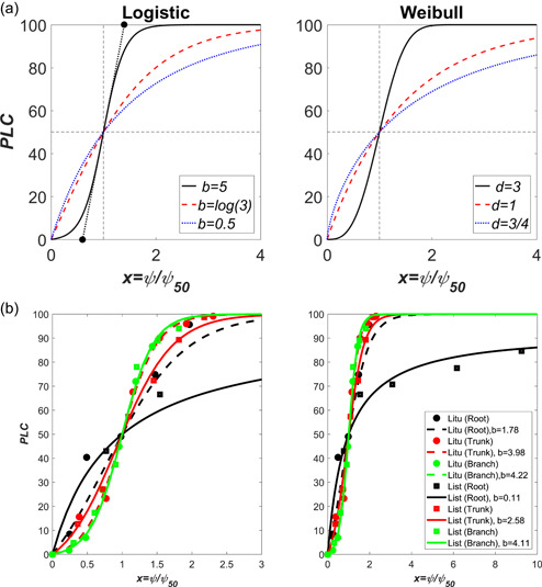
(a) Illustration of how r‐shaped and s‐shaped PLC curves emerge from the simplified logistic (left) and Weibull (right) models for embolism spread with constant b (left) and constant $d$ (right). For $b\le \log \mathrm{}\left(3\right)$, the logistic PLC resembles an r‐shaped function whereas for $b>\log \mathrm{}\left(3\right)$, the PLC is s‐shaped. Likewise, for $d\le 1$, the PLC resembles an r‐shaped function whereas for $d>1$, the PLC is s‐shaped. The two closed circles (left panel) is the extrapolation of the line ${\mathit{PLC}}_{\mathit{lin}}(x)$ to PLC= 0 (air entry) and PLC = 1 (runaway cavitation) and the determination of their associated normalized tension $x$ from b only. (b) The organ‐specific vulnerability curves for two species—Liriodendron tulipifera (Litu) and Liquidambar styraciflua (List) for normalized tension. The branch and trunk vulnerability curves are s‐shaped and similar (left) whereas the root vulnerability curve for List is r‐shaped (right). The left plot is shown over a restricted range of x to illustrate the collapse of branch and trunk level vulnerability curves for the logistic curve whereas the right plot is intended to illustrate the r‐shaped root vulnerability curve for List. [Color figure can be viewed at wileyonlinelibrary.com]

Figure 4.

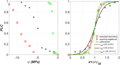
Left: Variations of measured xylem vulnerability curves (VC) across three species ranging from desert shrubs to riparian trees (data digitized by us from Sperry, 2000). Right: The percent loss of conductivity (PLC) variations for normalized xylem pressure ($x=\psi /{\psi }_{50}$) along with the logistic fit to them yielding the ease of cavitation spread parameter $b$. Note the approximate collapse of the measured VCs with $x$ on a single curve where the remaining shape differences can be explained by b. [Color figure can be viewed at wileyonlinelibrary.com]

A more complicated network model that considers embolism adjacency and membrane porosity for each pit field can be used to refine the estimate of $b$. When membrane porosity in each pit‐field is represented by a distribution of maximum pore sizes and when membrane stretching depends on x so that as the membrane stretches, maximal pores along the membrane become larger, a non‐constant $b$ emerges given by an extreme value distribution

$$b{k}_n=\frac{d}{c}{\left(\frac{x}{c}\right)}^{d-1},$$

where $c$ is a normalizing pressure that reflects the central pressure (63rd percentile of $k_n$) necessary for air entry into the biggest pores of the population of pit‐fields (bubble propagation pressure) and $d$ is an exponent related to the coefficient of variation of these maximum pores and thus the leakier pores in the aforementioned population of pit‐fields (i.e., the rare pit hypothesis, Christman et al., 2009).

Inserting this estimate into the simplified embolism spread model yields

$$\mathrm{PLC}=k_n=1-\exp \left[-{\left(\frac{x}{c}\right)}^d\right],$$

where $c={\left(0.693\right)}^{-1/d}$ when normalizing a $\mathrm{PLC}=0.5$ at $x=1$. For $d>1$, an s‐shape vulnerability curve emerges whereas for $d<1$, an r‐shape vulnerability curve emerges (see Box 2). Comparisons for PLC shapes for logistic and Weibull are discussed in Box 2.

4.1. Xylem hydraulics and the safety‐efficiency tradeoff

Plants have evolved a variety of strategies to prevent hydraulic failure in their conductive tissues while ensuring efficient water delivery to leaves. This hypothesis frames the ‘safety‐efficiency tradeoff’ or ‘runaway embolism’ versus ‘hydraulic sufficiency’ (Tyree & Sperry, 1989). This is the leading hypothesis that seeks to explain why multiple vulnerability curve shapes exist across different species and why species from different habitats can have such different vulnerability curves. Figure 4 shows the measured vulnerability curves for three different species—two desert shrubs and one riparian tree (Sperry, 2000). Clearly, the magnitude of ${\psi }_{50}$ is large for the desert shrubs and small for the riparian tree. When normalizing these measured PLC with ${\psi }_{50}$, the vulnerability curves roughly collapse on a single curve, and remaining differences between vulnerability curves can be captured by the ease of cavitation spread parameter b. The reported maximum conductance for the riparian tree is much larger than the desert shrub. This is the essence of the safety (i.e., ${\psi }_{50}$) versus efficiency (maximum conductance) tradeoff.

To illustrate the basic premise behind such tradeoff, whole plant‐scale assessment is required. It is thus assumed that the vulnerability curve (logistic or Weibull) represents the root‐xylem hydraulic conductivity. Transpiration $T_r,$ which measures the hydraulic capacity of the xylem to deliver water to satisfy the carbon demand of the plant for a preset leaf ${\psi }_l$ and root ${\psi }_r$ tension is given by

$$T_r=\frac{1}{h}{\int }_{{\psi }_r}^{{\psi }_l}K\left(\psi \right)d\psi ,$$

where h is the path length from root to leaf (surrogated to plant height), and $K\left(\psi \right)$ is the conductivity of the xylem at tension $\psi$. After some approximations (see Box 3), it can be shown that the maximum transpiration is given by

$$T_r\approx \frac{K_{\max }}{h}{\psi }_{50},$$

where $K_{\max }$ is the maximum hydraulic conductivity of the xylem. Because $K_{\max }$ is a measure of maximum hydraulic capacity (efficiency) and ${\psi }_{50}$ is a measure of safety against cavitation, the safety‐efficiency tradeoff emerges naturally from plant hydraulics. Thus, the same transpiration rate $T_r$ can be delivered via multiple strategies—from the efficient to the safe. In this derivation, it was assumed that $|{\psi }_r/{\psi }_{50}|<<1$, $|{\psi }_l/{\psi }_{50}|>>1$ and $b>>1$. It is to be noted that empirically establishing an inverse relation between $K_{\max }$ and ${\psi }_{50}$ without the additional constraint set by maximal $T_r$ (that varies by tree size, climatic conditions, etc.) cannot be used to support or negate safety‐efficiency tradeoffs given the large variations in maximum transpiration as shown in Box 3 across many species.

Box 3: Maximum transpiration, safety‐efficiency tradeoff and hydraulic segmentation.

Maximum transpiration: In the derivation of maximum transpiration here, the vulnerability curve is assumed to be a logistic function set by its approximate form

$$\frac{K\left(\psi \right)}{K_{\max }}=\frac{1}{1+\exp \left[b(x-1)\right]},$$

where $x=\psi /{\psi }_{50}$ and the interpretation of $b$ is as before. This function captures much of the non‐linearities expected in the Weibull shaped vulnerability curve (see Box 2) but permits analytical tractability without resorting to any special mathematical functions.

As noted earlier, $K\left(0\right)/K_{\max }$ < 1 in this vulnerability curve representation due to the need for a finite number of cavitated vessels to initiate embolism spread by air seeding. With this approximated vulnerability curve, the transpiration $T_r$ can be expressed as follows:

$$T_r=\frac{1}{h}{\int }_{{\psi }_r}^{{\psi }_l}K\left(\psi \right)d\psi =\frac{K_{\max }}{h}{\psi }_{50}\left[\frac{{\psi }_l-{\psi }_r}{{\psi }_o}+\frac{1}{b}\log \left(\frac{1+e^{b({\psi }_r/{\psi }_{50}-1)}}{1+e^{b({\psi }_l/{\psi }_{50}-1)}}\right)\right].$$

To further simplify, let $|{\psi }_r/{\psi }_{50}|<<1$ so that

$$T_r=\frac{K_{\mathit{max}}}{h}{\psi }_{50}\left[\frac{{\psi }_l}{{\psi }_{50}}+\frac{1}{b}\mathit{log}\left(\frac{1+e^{-b}}{1+e^{b({\psi }_l/{\psi }_{50}-1)}}\right)\right].$$

Safety‐efficiency tradeoff: When $|{\psi }_l/{\psi }_{50}|>>1 \text{and }b>>1$, then $T_r$ attains only an asymptotical maximum given by

$$T_r=\frac{K_{\max }}{h}{\psi }_{50}\left[\frac{{\psi }_l}{{\psi }_{50}}+\frac{1}{b}\log \left(e^{-b({\psi }_l/{\psi }_{50}-1)}\right)\right]=\frac{K_{\max }}{h}{\psi }_{50}.$$

This limit shows the origin of the so‐called ‘safety‐efficiency’ tradeoff between maximum conductance ($K_{\max }/h$) and a measure of resistance to cavitation ${\psi }_{50}$. This tradeoff appears to be independent of $b$ but only in the limit when $|{\psi }_l/{\psi }_{50}|>>1,b>>1$ (s‐shaped vulnerability curve). Sperry (2000) showed that $T_r$ attains an asymptotic maximum with increasing ${\psi }_l$ and that ${\partial T}_r/\partial {\psi }_l>0$ at all leaf tensions. This result is now contrasted to an alternative finding by Manzoni et al. (2013) based on hydraulic segmentation.

Hydraulic segmentation: The hydraulic segmentation vulnerability hypothesis suggests that distal portions of the plant (e.g., leaves) should be more vulnerable to embolism than trunks. The original argument was based on carbon economy of the plant and implies that non‐redundant organs (e.g., trunks) require a massive carbon investment when compared to leaves (Zimmermann, 1983). A hydraulic (instead of a carbon investment) explanation can also be offered based on the stability analysis of embryonic bubbles. The stability of embryonic bubbles is linked to background xylem tension as earlier discussed. The higher the background xylem tension, the more unstable the bubbles are and the more prone they are to explosion and embolizing vessels. Based on cohesion‐tension theory, this tension is largest next to leaves – at least when compared to the trunk, and this is the idea behind the original hydraulic segmentation hypothesis (Zimmermann, 1983). The immediate consequence of this result is that leaf xylem tension may be limiting the operating pressure of the xylem. Some evidence across many species has been offered (Johnson et al., 2016; Tsuda & Tyree, 1997; Tyree et al., 1993).

Using this interpretation, Manzoni et al. (2013) considered the maximum transpiration estimate with the limiting approximation $K(\psi )~K\left({\psi }_l\right)$ so that

$$T_r=\frac{1}{h}{\int }_{{\psi }_r}^{{\psi }_l}K\left(\psi \right)d\psi ~K({\psi }_l)\left(\frac{{\psi }_l-{\psi }_r}{h}\right),$$

where the symbol ‘~’ indicates scales as or proportional to. Using the same logistic function with $x={\psi }_l/{\psi }_{50}$ and upon ignoring root tension compared to leaf tension, $T_r$ reduces to

$$T_r=\frac{K\left({\psi }_l\right)}{h}{\psi }_l=\frac{K_{\max }{\psi }_{50}}{h}\frac{x}{1+\exp \left[b(x-1)\right]}.$$

As ${\psi }_l$ (or $x$) increases, the (linear) driving force for transpiration increases but the non‐linear $K({\psi }_l)$ decreases. Manzoni et al. (2013) demonstrated that a maximum transpiration must then exist and can be determined from

$$\frac{{\partial T}_r}{\partial {\psi }_l}=0=\frac{K_{\max }}{h}{\psi }_{50}\frac{[1+(1-\mathit{bx})\text{exp}\left(b(x-1)\right)]}{{[1+\text{exp}\left(b(x-1)\right)]}^2}=0.$$

A solution of this algebraic equation for $x$ can be expressed in closed form as follows

$$x_m=\frac{{\psi }_l}{{\psi }_{50}}=\frac{1+\mathit{W}\left[\text{exp}(b-1)\mathbf{\right]}}{b},$$

where $\mathit{W}\mathbf{[}\mathbf{.}\mathbf{]}$ is the Productlog or the principal Lambert W‐function that arises frequently in mathematical solutions of the susceptible‐infectious‐recovery [SIR] model in epidemiology as recently reviewed elsewhere (Katul et al., 2020). Its value is given by the alternating series

$$\mathit{W}[\mathit{u}]=u-u^2+\frac{3}{2}{u}^3-\frac{8}{4}{u}^4+\frac{125}{24}{u}^5-\text{…},$$

and the corresponding maximum transpiration at $x_m$ is given by

$$T_r=\frac{K\left({\psi }_l\right)}{h}{\psi }_l=\frac{K_{\max }{\psi }_{50}}{h}\zeta \left(b\right)\mathrm{;}\zeta \left(b\right)=\frac{x_m}{1+\exp \left[b(x_m-1)\right]}.$$

A comparison of the two transpiration solutions, the continuous distribution of tension versus tension set by the most distal organ—the leaf, is featured in Figure B3. Unsurprisingly, the hydraulic segmentation argument yields a lower maximum transpiration due to the fact that ${\psi }_l$ restricts water transport across the entire xylem (Figure B3). This reduction from the maximum predicted by the continuous description is captured by $\zeta (b)<1.$ More significant is that the two solutions differ fundamentally in how they predict normalized transpiration to vary with normalized leaf tension. In the hydraulic segmentation limit, ${\partial T}_r/\partial {\psi }_l=0$ exists at a unique leaf tension $x_m$ whereas in the continuous xylem tension case, it does not. Hence, the continuity of xylem tension and its variability within the plant must be accommodated in hydraulic representation of the soil–plant system. A logical follow‐up question to ask is how well $K_{\max }{\psi }_{50}{h}^{-1}$ recovers maximum transpiration in trees. The data set used in Manzoni et al. (2013) is revisited and comparisons between reported and predicted maximum transpiration from $K_{\max }{\psi }_{50}{h}^{-1}$ is shown in Figure B3. Agreement between measured (abscissa or x) and predicted (ordinate or y) maximum transpiration rates in the figure can be summarized by the regression model $\log \left(y\right)=0.68\log \left(x\right)-0.304$ with a coefficient of determination $R^2=0.74$. These regression statistics and their statistical interpretation must be treated with caution given that the plant hydraulic traits and the maximum transpiration were not measured at the same geographic locations and not at the same organ scale (transpiration was measured using sapflow). Last, both—hydraulic segmentation and the continuous xylem tension arguments agree that a safety‐efficiency tradeoff must exist between maximum xylem conductance ${(K}_{\max }{h}^{-1})$ and ${\psi }_{50}$ when constrained at the same maximum transpiration.

Figure B3.

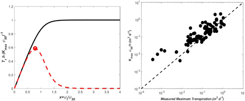
Left panel: Comparison between normalized transpiration $T_{r}h{\left(K_{\max }{\psi }_{50}\right)}^{-1}$ against normalized leaf tension $x={\psi }_l/{\psi }_{50}$ for the continuous tension distribution across the entire root‐xylem system (black solid) and the hydraulic segmentation limit where leaf tension dominates the entire hydraulic conductivity (red dashed). The same vulnerability curve is used in both calculations ($b=5$). In the latter case, a clear maximum transpiration emerges (open circle) at $x_m$ whereas in the continuous xylem tension case, it does not. Right panel: comparison between measured and modelled maximum transpiration (=$K_{\max }{\psi }_{50}{h}^{-1}$) multiplied by sapwood area over three orders of magnitude. The one‐to‐one line is also shown (dashed). The analysis is suggestive that a safety‐efficiency tradeoff can emerge between $K_{\max }$ and ${\psi }_{50}{h}^{-1}$ (i.e., a hydraulic gradient) when conditioned on maximum transpiration (coefficient of determination = 0.74). When the analysis is repeated per unit sapwood area, the conclusions are unaltered though the scatter is somewhat larger. The data set includes the following species: Acer saccharum, Betula papyrifera, Carapa procera, Cecropia longipes, Eucalyptus grandis, Eucalyptus regnans, Eucalyptus saligna, Fagus sylvatica, Larix cajanderi, Larix gmelinii, Liquidambar styraciflua, Liriodendron tulipifera, Picea mariana, Pinus banksiana, Pinus pinaster, Pinus radiata, Populus tremuloides Populus Sp., Pseudotsuga menziesii, Salix matsudana, Quercus alba, Quercus rubra, and Quercus petraea. [Color figure can be viewed at wileyonlinelibrary.com]

The link to the VBE and other climatic factors can now be made explicit when noting that

$$P_g=\mathrm{WUE}\frac{T_r}{L}=\left[1.6\frac{c_a}{\mathrm{VPD}}\left(1-\frac{c_i}{c_a}\right)\right]\frac{K_{\max }}{\mathit{hL}}{\psi }_{50}\left[,\times ,[,\frac{{\psi }_l}{{\psi }_{50}}+\frac{1}{b}\log \left({\mathrm{e}}^{-b({\psi }_l/{\psi }_{50}-1)}\right)\right],$$

where $P_g$ is, as before, aboveground photosynthesis, $\mathrm{WUE}$ is the leaf‐scale water use efficiency, $c_a$ and $c_i$ are atmospheric and intercellular CO₂ concentrations, respectively, $\mathrm{VPD}$ is the vapour pressure deficit that depends on the saturation vapour pressure (and thus temperature) and relative humidity in the atmosphere, and $L$ is as before the leaf area. Numerous theories, including those based on stomatal optimization, reasonably predicted $\mathrm{WUE}$ from the aforementioned drivers (e.g., Katul et al., 2010).

5. CELL WALL MECHANICS

Large bubbles in an embolized vessel or tracheid are restricted in size by cell wall mechanics and pit membrane properties. The mathematical description of such interactions between cell walls and bubbles remains fraught with difficulties though catastrophe theory can make qualitative and general statements about such interactions. For simplicity, the case where pits rapidly close so as to isolate an intact from an embolized tracheid is first considered for illustration in Box 4. Such pits approximate the torus margo (mainly in conifers): the torus is a thickened central portion that is attached to a porous margo (Figure 1g; Domec et al., 2006; Dute, 2015). It is shown here that the inclusion of cell wall mechanics switches the previously studied catastrophe in bubbles in Section 3 from ‘fold' to ‘cusp' as represented by the bifurcation diagrams in Box 4. Those diagrams reveal the genesis of a cusp catastrophe surface along the initial (or background) xylem pressure and number of air molecules $n_a$introduced into the bubble. The switch from fold to cusp catastrophe arises because cell wall mechanics act to restrict the maximum bubble size (assuming perfect isolation of the tracheid) that is stable as long as the torus margo isolates the embolized tracheid. This bubble size restriction results in a new equilibrium bubble size (compared to ones derived in Section 3) that depend on processes governed by cell wall mechanics and water compression instead of surface tension and gas pressure within the bubble. This new equilibrium radius (see Box 4) is stable and given by

$$R={\left[\frac{-3}{4\pi }{p}_s(\kappa +\mu )V_o\right]}^{1/3},$$

where $V_o$ is the initial volume of the tracheid, $\mu$ is related to cell‐wall material (in Box 4) and $\kappa$ is the water compressibility coefficient. The new equilibrium is independent of $n_a$ and surface tension. The similarity between the cusp catastrophe discussed in Box 4 and the one derived for the spruce‐budworm outbreak (Ludwig et al., 1978) is rather striking. In the case of the spruce‐budworm, the worm population is driven by the imbalance between a logistic growth and predation (mainly due to birds) represented by a sigmoidal function (known as type‐III Holling predation function). Depending on the variations in the two control parameters, the worm population has two stable equilibria (refuge and outbreak) and an unstable equilibrium point that is an intermediate between the two stable equilibria. The harmless bubbles are analogous to the ‘refuge' state of the worm whereas embolism is analogous to ‘outbreak' and thus catastrophe (or hydraulic failure of the xylem).

Box 4: Embolism and cell wall mechanics: A shift from the fold to cusp catastrophes.

Section 3 established necessary conditions for bubble size instability when xylem liquid pressure was assumed unaltered (small embryonic bubbles). As a bubble becomes unstable and begins to expand, the torus margo shuts rapidly isolating the intact tracheid from the embolized one. Thus, the liquid tension can no longer be assumed constant. Moreover, the tracheid volume sets an upper constraint on the bubble size. The analysis here shows how the inclusion of these two effects alters the nature of the catastrophe within the tracheid. The starting point here is to assume the xylem liquid pressure $p_s$ before embolism occurs is the same for two adjacent intact tracheids. After embolism commences in one of them, $p_s$ is assumed to represent the intact tracheid pressure only. A large and saturated bubble of radius $R$ carrying $n_a$ air and water vapour molecules is now considered. For large bubbles, the liquid pressure in an isolated embolized tracheid must increase or liquid tension must be reduced because water molecules are being pushed together in the now sealed tracheid. The contracting force acting on this large bubble of surface area ($4\pi R^2$) is only surface tension whereas the expanding forces are, as before, xylem pressure $p$ (negative) and the gas pressure within the bubble. At equilibrium, a force balance between contracting and expanding forces reduces to (Konrad & Roth‐Nebelsick, 2006)

$$8\pi \gamma R+4\pi R^{2}p-\frac{3\mathfrak{R}T{n}_a}{R}=0,$$

where the first, second, and third terms represent the surface tension, xylem pressure $p$, and gas pressure due to air and water vapour molecules as in Section 3. When $p=p_s,$ the analysis reduces to the one earlier described with the assumption that no pressure differential exists to close the pit membrane between intact and embolized vessel. This case is labelled as the ‘small‐bubble’ scenario because the bubble volume is presumed to be sufficiently small compared to the vessel volume so as not to impact the background xylem pressure. It leads to the fold catastrophe earlier mentioned in Figure 2. For larger bubbles, deviations between $p(>p_s)$ and $p_s$ occur and are thus responsible for rapidly closing the pit membrane ensuring hydraulic isolation between embolized and intact tracheid. To proceed further and bring into focus a connection between cell wall mechanics and embolism, a relation between $p$ and $p_s$ is required within the embolized tracheid. A simplified version of the approach in Konrad and Roth‐Nebelsick (2006) is now followed to arrive at this relation. In this revised approach, the cell walls are assumed to be elastic, and the expanded bubble volume must be accompanied by (i) an expansion in tracheid volume, (ii) a reduction in the xylem water tension for some water trapped inside the tracheid, and (iii) some water volume escaping before torus shut‐down. Defining the undeformed tracheid volume as $V_o$ and assuming $V_o$ is initially full of water, the change in tracheid volume due to the presence of large bubbles is $∆V=(4/3)\pi R^3$ and can be related to the cell‐wall material compressibility $\mu$ using

$$\mu =\frac{∆V}{V_o}\frac{1}{p-p_s}.$$

The liquid pressure $p$ after embolism is now

$$p-p_s=\frac{1}{(\mu +\kappa )}\frac{1}{V_o}\frac{4}{3}\pi R^3,$$

where $\kappa =5\times {10}^{-10}$ Pa^‐1 is the coefficient of compressibility of water. The $p_s$ represents both the liquid pressure (i.e., negative) before embolism and the liquid pressure in the intact tracheid. Once $\mathit{|p}-p_s|$ exceeds a small threshold (or the bubble size exceeds a threshold), the torus closes and ensures hydraulic isolation (Schulte & Hacke, 2021) thereby trapping some water and air. Beyond this point, the torus is assumed to remain intact and no ‘air‐seeding’ occurs. Inserting this result into the force balance at equilibrium leads to

$$8\pi \gamma R+4\pi R^2\left[p_s+\frac{1}{(\mu +\kappa )}\frac{1}{V_o}\frac{4}{3}\pi R^3\right]-\frac{3\mathfrak{R}T{n}_a}{R}=0.$$

This equation can be rearranged as a sextic (order 6) polynomial in bubble radius $R$ that is given by

$$\left[\frac{1}{(\mu +\kappa )}\frac{1}{V_o}\frac{16}{3}{\pi }^2\right]R^5+4\pi {p_{s}R}^2+8\pi \gamma R-\frac{3\mathfrak{R}T{n}_a}{R}=0.$$

There are no exact solutions for such a polynomial equation. Konrad and Roth‐Nebelsick (2006) considered ‘asymptotic’ cases and showed that for large $R$, the last two terms in the force balance can be ignored leading to

$$\frac{R}{{V_o}^{1/3}}={\left[\frac{-3}{4\pi }{p}_s(\mu +\kappa )\right]}^{1/3}.$$

This dimensionless ‘large radius’ equilibrium is stable and independent of surface tension and number of air molecules. It only depends on the xylem tension before embolism, water and cell wall compressibility. To link $\mu$ to common material properties, the tracheid is assumed to be cylindrical with wall thickness $d_t$, undeformed radius $r_t$ and length $l_t$, with a Poisson number ${\sigma }_t$ and Young's modulus of elasticity $E_t$. In this case, Konrad and Roth‐Nebelsick (2006) showed that $\mu$ depends on the structural and undeformed geometric properties of the tracheid and is given by

$$\mu =\left(\frac{2r_t}{d_t}\right)\left[\frac{1-{{(\sigma }_t)}^2}{E_t}\right].$$

It is noted that $R$ scales as ${(\mu +\kappa )}^{1/3}$, which makes $R$ insensitive to small variations in $E_t$ or ${\sigma }_t$. When $V_o=\pi {r_t}^2{l}_t$, the ratio between the radii of the large bubble and the tracheid is given by

$$\frac{R}{r_t}={\left\{\frac{-3}{2}{p}_s\left(\frac{l_t}{d_t}\right)\left[\frac{1-{{(\sigma }_t)}^2}{E_t}\right]\right\}}^{1/3}.$$

For a coniferous tracheid with ${\sigma }_t=0.5$, $E_t$ = 10⁴ MPa, $l_t/d_t=4\times {10}^3$, and $p_s=-1$ MPa, $R/r_t$ = 0.77. An $E_t$ = 8–10 GPa has been reported for cell walls for Albizia julibrissin, Acer negundo, and Pinus taeda (Domec et al., unpublished data). The $E_t$ for the torus margo membrane (compared to cell walls), which constitutes only a small fraction of the tracheid surface area (Domec et al., 2006), are an order of magnitude smaller ranging from 0.012 GPa in P. taeda to 0.4–0.9 GPa in A. julibrissin and A. negundo (and their effects are ignored). The analysis here suggests that the bubble radius expands to a maximum of 0.77 the tracheid radius, and thus embolism does not entirely replace all the water with air. Given the small compressibility of water, the remaining water trapped within the tracheid does not change its volume. Hence, the water that must have escaped the tracheid before closure of the torus can be computed from the volume imbalances. That is, the final volume of the expanded tracheid less bubble volume is the water part trapped, which can then be normalized by $V_o$ to assess the fractional volume of water that escaped before the torus shuts. The remaining trapped water within the isolated tracheid is at a reduced tension with $|p|<\left|p_s\right|$. This trapped water can play an under‐appreciated role in bubble dissolution (unless the torus membrane fails because of structural fatigue or large pressure differential across it).

Returning to the small $R$ case, the first term in the force balance can be ignored thereby recovering the previous findings about bubble dynamics. That is, the force balance is now governed by the cubical equation

$$4\pi {p_{s}R}^2+8\pi \gamma R-\frac{3\mathfrak{R}T{n}_a}{R}=0.$$

Two positive real roots only exist when $n_a<n_{\max }$, where $n_{\max }$ is given as before in the bubble scale equations

$$n_{\max }=\frac{2\pi \gamma }{\mathfrak{R}T}{\left(\frac{8\gamma }{9p_s}\right)}^2.$$

The two roots corresponding to one unstable and one stable equilibrium (i.e., a fold catastrophe) are associated with saddle‐node bifurcation. The bifurcation diagram with respect to the two control variables $p_s$ and $n_a$ is featured in Figure B4 for the analytical results in the limit of large and small radii for the sextic equation. The existence of an unstable branch between two otherwise stable equilibrium radii is indicative of a hysteretic behaviour in bubble dynamics when the control variables change as shown in Figure B4. To illustrate, a bubble with initial radius of ${10}^{-2}$  $\mathrm{\mu m}$ at a fixed $p_s=-5$ MPa and $n_a=1\times {10}^{-20}$ mol will follow the embolism trajectory towards the large radius equilibrium as shown in Figure B4. To bring back this bubble to its initial size (at constant $n_a)$ requires a reduction in $p_s$ to −2 MPa. When this state is reached (i.e., recovering its initial radius), the bubble will proceed to follow the path towards the low radius stable equilibrium branch shown by the hysteresis loop in Figure B4. For reference, the saddle node bifurcation point is also featured on the surface. The sextic equation here can be reduced to a cubic equation by setting $R^2$ to a new state variable. This reduced sextic equation experiences symmetry breaking due to (i) the presence of non‐integer exponents and (ii) a so‐called imperfection parameter (=$3\mathfrak{R}T{n}_a$) that depends only on one of the control variables (=$n_a$). A similar cubic system but without non‐integer exponent was derived for the spruce‐budworm (Ludwig et al., 1978). The harmless bubbles are analogous to the ‘refuge’ state of worm (from bird predation) whereas embolism is analogous to ‘outbreak’ and thus hydraulic failure (or catastrophe).

Figure B4.

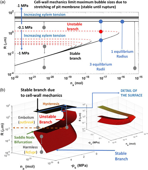
(A) Bifurcation diagram shown in two‐dimensions (equilibrium bubble radius R vs. $n_a$) with variations in $p_s$ featured as multiple curves instead of a separate dimension illustrating the genesis of a cusp catastrophe. The equilibrium points are derived from the simplified sextic equation in the limit of large and small radii. The large radii equilibria corresponding to embolism are shown as horizontal lines. Note that this large R equilibria are independent of $n_a.$ The remaining two equilibria only exist for $n_a<n_{\max }$, where $n_{\max }$ decreases with increasing $p_s$. (b) Bifurcation diagram obtained by numerically solving the sextic equation at equilibrium when net forces acting on the bubble are in balance. This diagram reveals the cusp catastrophe surface along the two control parameters: initial (or background) xylem pressure and number of air molecules introduced into the bubble. The diagram resembles the cusp catastrophe studied for the spruce budworm dynamical system. The lower equilibrium radii forming the stable branch delineates harmless bubbles (resembling the refuge zone in the spruce budworm system) and the large radii stable equilibrium branch delineates embolism (associated with outbreak for the spruce budworm system). The saddle node bifurcation that forms in the absence of cell‐wall mechanics constraints (see Section 3) and the hysteresis loop along the cusp surface are also shown. Note that the radii associated with the upper stable branch are not sensitive to the number of air molecules except at very low xylem pressure (see detail). [Color figure can be viewed at wileyonlinelibrary.com]

6. THE CANOPY UNDERGROUND

Most studies linking stomatal regulation to plant hydraulics focus on xylem vulnerability as the primary constraint on water flow while neglecting the explicit role of soil hydraulic conductivity but with several exceptions (Binks et al., 2022; Huang et al., 2017; Manoli et al., 2017; Mrad et al., 2019; Siqueira et al., 2008; Williams et al., 2001). The hydraulic conductivities of the xylem of the different plant organs (leaves, branches, stem and roots) and of the soil are variable and discerning the ‘bottleneck’ to water movement remains a formidable challenge. The radial conductance of the root is also variable and impacted by root surface area as well as by the expression and activity of aquaporins (Chaumont & Tyerman, 2014; Ehlert et al., 2009). The question that appears is ‘What are the primary constraints that regulate water flow across the soil‐plant continuum?’ An answer to this long‐standing question requires methods to measure and partition the hydraulic conductance of the different elements of soil–plant system that are now beginning to proliferate in plant hydraulics (Johnson et al., 2016; McCulloh et al., 2019).

Water loss at leaves depends on continuous supply of water in the xylem from the soil to absorbing roots (Passioura, 1988), which is often described as analogous to Ohm's and Kirchhoff's laws (Sperry et al., 1998). Applying these laws to plants, the water flow depends on water potential gradients and the resistance of pathways of soil–plant continuum. Under wet soil conditions, the soil hydraulic conductivity is presumed to be sufficient to sustain transpiration but in drier soils, the soil can become the limiting factor for water flow into the roots as its hydraulic conductivity decreases below that of roots (Carminati & Javaux, 2020; Draye et al., 2010; Sperry et al., 2017). It is these conditions and their potential to switch the controls on transpiration from plant to soil (i.e., a tipping point) that motivate the inclusion of this section in a plant‐hydraulics review.

The xylem network of overlapping conduits extends to the roots where the negative root pressure pulls water from the soil pores (Steudle, 1994). Not surprisingly, root hairs have evolved to allow the plant to take in as much water and minerals from the soil as possible. Whereas leaves maximize carbon gain for a given loss of water (Givnish & Vermeij, 1976; Sperry et al., 2017), roots perform the converse optimization—maximize water and nutrient uptake for a given investment in carbon for root construction (Guswa, 2008). Water and dissolved minerals from the soil move into the root hairs by osmosis and travel into the xylem found in the root, where they are transported to the rest of the plant.

As in the leaves, there is a symplastic and apoplastic water pathway from the root hairs and across the root cortex. Then, at the root endodermis that represents a single layer of cells bordering the cortex, water is forced by reverse osmosis through cell membranes because of the Casparian strip that forms an apoplastic barrier. Under saturated soil and low transpiration, ions accumulate in the root xylem thus allowing water to move into root xylem by osmosis (Tibbetts & Ewers, 2000). During dry‐down, the soil is rarely near saturation. Soil water is usually under a negative pressure because like in plant xylem, capillary forces hold water between soil particles (Figure 5). The cohesion–tension mechanism at the soil–root interface represents a ‘tug‐of‐war on a rope of water’ between capillary forces in cell walls and capillary forces in soil. In dry soil, plants have to pull against soil water potentials of −1 MPa or lower because water is now being stored in ever smaller and smaller soil pores (<0.15 $\mathrm{\mu m}$). Water stored in large pores is already extracted as this water requires far less tension (or work by the plant) to extract. In addition, because of the reverse osmosis at the root, the xylem must extract water not only from the soil pore space, but also against the osmotic strength of the soil solution. If the loss of soil hydraulic conductivity occurs at water potentials less negative than xylem pressure thresholds, then xylem vulnerability and xylem hydraulics is not the main determinant of transpiration (Körner, 2019; Sperry et al., 1998).

Figure 5.

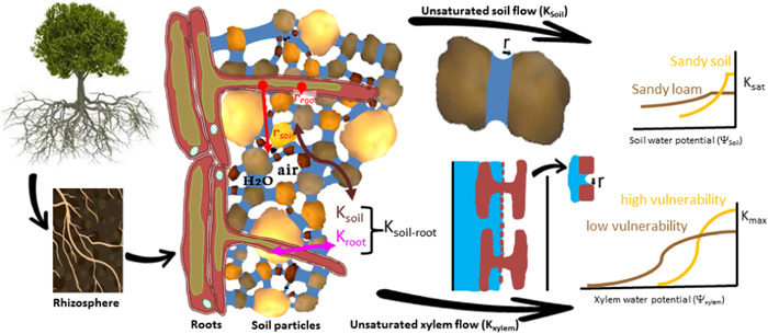
A conceptual representation of the contributions and the changes in soil (K _soil) and root hairs (K _root) hydraulic conductivity to rhizosphere conductance (K _soil‐root). Water (blue) in soil is held by capillary forces in pore space (radius r) under negative pressure due to surface tension. As soil dries, the soil water potential ($\mathrm{\psi }$ _soil ) becomes more negative and air replaces the water‐filled pore space (i.e., degree of saturation becomes smaller). Consequently, soil conductivity at saturation (K _sat) declines rapidly with $\mathrm{\psi }$ _soil dependently of soil texture, with sandy (porous soils) having higher K _sat, and being more sensitive to $\mathrm{\psi }$ _soil than for example sandy loam. Similarly, water in root xylem is also held at the interface of inter‐conduit pits by capillary forces and as xylem water potential ($\mathrm{\psi }$ _xylem) decreases air‐seeding occurs (Figure 1e), leading to an embolized conduit whose hydraulic conductivity declines from its maximum or fully hydrated values (K _max). Roots with high vulnerability to embolism have generally higher K _max, but analogous to porous soils, are also more sensitive to negative $\mathrm{\psi }$ _xylem than roots with low vulnerability because of larger pit membrane pores. r _root and r _soil are root radius and the radial distance from the centre of the roots to the mean distance between roots, respectively. [Color figure can be viewed at wileyonlinelibrary.com]

Belowground hydraulic failure outside of the xylem has been associated with some tree mortality events during severe droughts (Johnson et al., 2018). A number of modelling studies indicated that the most likely hydraulic failure point was in the rhizosphere (Domec et al., 2012; Huang et al., 2017; Mrad et al., 2019; Siqueira et al., 2008). In fact, plants are built to minimize the possibility of belowground hydraulic failure. For example, in loblolly pine trees growing on sand versus loam, xylem vulnerability to embolism was greater on loam even though sand is considered drier (Hacke et al., 2000). However, the pines produced xylem that was representative of the extraction limit for water in each soil type. There is no need to build highly resistant xylem if the soil that the plant is growing in has a high (less negative) extraction limit. Having overbuilt xylem in the sand would only lead to hydraulic dysfunction in the rhizosphere. These empirical results provide tantalizing clues that some coordination between soil and xylem hydraulics must exist. If so, this coordination may be exploited to assess ‘tipping points’ in terms of soil water tension where a switch from plant to soil hydraulics limit overall transpiration. Before doing so, key definitions and simplifications are needed.

6.1. Soil–root hydraulics

Plant water supply function (transpiration vs. leaf or soil water potentials) models now use soil‐to‐leaf (whole plant) vulnerability curves in concert with the soil‐to‐leaf hydraulic conductance to water flow (Johnson et al., 2016; Sperry & Love, 2015). In its simplest representation, soil to leaf hydraulic conductance (K _soil‐leaf) can be viewed as the result of two conductances in parallel (or two resistances in series). The first is K _soil‐root and represents the water‐potential‐dependent decrease in rhizosphere (i.e., the volume of soil water adjacent to the plant roots) conductance (Figure 5), and the second is K _root–leaf and represents the hydraulic conductance of the whole plant system (i.e., from the roots to the leaves). Each organ axial conductivity (K _root, K _trunk, K _branch and K _leaf) constituting K _root–leaf can decrease from its initial conductivity at full saturation to account for the loss of hydraulic conductivity (vulnerability curves; Figures 3 and 4).

Further, K _soil‐root can be decomposed into two components: $K_{\mathrm{soil},\mathrm{effective}}\left({\psi }_{\mathrm{soil}}\right)$ and $K_{\mathrm{root}}\left({\psi }_{\mathrm{root}}\right)$. The $K_{\mathrm{root}}$ represents the radial root conductance that varies with root water potential ${\psi }_{\mathrm{root}}$ and $K_{\mathrm{soil},\mathrm{effective}}$ is the effective soil hydraulic conductance characterizing the ease of water flow from the soil pores to a given surface area of root (A _root = 2πr _root L _root, where r _root is root radius, and L _root is root length) at soil water potential ${\psi }_{\mathrm{soil}}$. This effective soil conductance can be related to the commonly used soil hydraulic conductivity function $K_{\mathrm{soil}}\left({\psi }_{\text{soil}}\right)$ using (Nobel & Cui, 1992)

$$\frac{K_{\mathrm{soil},\mathrm{effective}}\left({\psi }_{\text{soil}}\right)}{K_{\mathrm{soil}}\left({\psi }_{\text{soil}}\right)}=\frac{A_{\text{root}}}{r_{\text{root}}\ln \left(\frac{r_{\text{soil}}}{r_{\text{root}}}\right)},$$

where $K_{\mathrm{soil}}\left({\psi }_{\text{soil}}\right)$ describes the decline in saturated soil hydraulic conductivity ($K_{\mathrm{sat}}$; Figure 5) in response to a decline away from the root at ${\psi }_{\mathrm{soil}}$. The $K_{\mathrm{soil}}\left({\psi }_{\text{soil}}\right)$ can be parameterized using several empirical power‐law functions (Brooks & Corey, 1964; Campbell, 1985; van Genuchten, 1980) with the simplest being

$$K_{\mathrm{soil}}=K_{\mathrm{sat}}{\left(\frac{{\psi }_{\mathrm{soil},a}}{{\psi }_{\mathrm{soil}}}\right)}^{2+3/\beta },$$

where ${\psi }_{\mathrm{soil},a}$ is the water potential near saturation and $\beta$ is the curvature parameter of the soil water retention curve. When the soil particle size distribution is described by power‐laws (i.e., fractal), there is theoretical support for this assumed empirical shape from percolation theory (Hunt, 2005). Expressing A _root and L _root on a ground area basis provides an estimate of an effective path length formed by the ratio of conductance to conductivity at the same${\psi }_{\text{soil}}$ and given as

$$\frac{K_{\mathrm{soil},\mathrm{effective}}\left({\psi }_{\text{soil}}\right)}{K_{\mathrm{soil}}\left({\psi }_{\text{soil}}\right)}=\frac{\text{RAI}}{r_{\text{root}}\log \left(\frac{r_{\text{soil}}}{r_{\text{root}}}\right)},$$

where RAI is the root area index, and r _soil is the radial distance from the centre of the roots to the mean distance between roots (Campbell, 1985; Doussan et al., 1998).

In this expression, it is assumed that each root is a cylinder uniformly spaced and therefore r _soil = (π RLD)^−1/2, where RLD is the root length density (total length of roots per unit of soil volume). Quantifying canopy versus root effects on plant hydraulics is often conducted by setting the ratio of projected leaf area index (LAI) to all‐sided RAI = 2πr _root l _rz RLD, where l _rz is the rooting depth, and r _root ranges from 80 to 100 μm for unsuberized fine roots and from 5 to 10 μm for root hairs (Dittmer, 1949). Most water and nutrients are absorbed by root hairs, cells formed on the epidermis of the region of root maturation. In most angiosperms and some conifers, root hairs often form on fine roots and thus increase their effective absorbing surface area (McCully, 1999). Because root hair diameter and above all root hair length are difficult to determine due to their fragile and unicellular structure, most root area values are based on fine roots and should be replaced by fine root diameter that is typically around 100 μm. With these definitions, the consequences of a soil–plant coordination conjecture to hydraulic controls on transpiration are explored using an equilibrium analysis between maximum soil supply and maximum plant demand for water.

6.2. Tipping points and coordination between soil and plant controls on transpiration

In Box 3, the transpiration $T_r$ was related to the root–leaf xylem vulnerability curve by

$$T_r=\frac{1}{h}{\int }_{{\psi }_r}^{{\psi }_l}K\left(\psi \right)d\psi =\frac{K_{\max }}{h}{\psi }_{50}\left[\times ,[,\frac{{\psi }_l-{\psi }_r}{{\psi }_{50}}+\frac{1}{b}\log \left(\frac{1+{\mathrm{e}}^{b({\psi }_r/{\psi }_{50}-1)}}{1+{\mathrm{e}}^{b({\psi }_l/{\psi }_{50}-1)}}\right)\right].$$

Because this $T_r$ is governed by leaf pressure ${\psi }_l$ and partly dictated by the carbon demand of the plant, we label this transpiration rate as ‘demand‐controlled transpiration’. When $|{\psi }_l/{\psi }_{50}|\gg 1 \text{and }b\gg 1$, $T_r$ attains a maximum at ${K_{\max }\psi }_{50}/h$ as earlier derived.

For the soil system, the ability of the soil to supply water to the roots is given by

$$T_{\mathrm{supply}}=\frac{\text{RAI}}{r_{\mathrm{root}}\log \left(\frac{r_{\mathrm{soil}}}{r_{\mathrm{root}}}\right)}{\int }_{\psi \mathrm{soil}}^{{\psi }_r}{K}_{\mathrm{soil}}\left(\psi \right)d\psi .$$

With this formulation, the ability of the soil to supply water to the roots is given by

$$T_{\mathrm{supply}}=\frac{\text{RAI}}{r_{\mathrm{root}}\log \left(\frac{r_{\mathrm{soil}}}{r_{\mathrm{root}}}\right)}\left(\frac{\beta }{\beta +3}\right)K_{\mathrm{sat}}{\psi }_{\mathrm{soil},a}\left[\times ,[,{\left(\frac{{\psi }_{\mathrm{soil},a}}{{\psi }_{\mathrm{soil}}}\right)}^{1+3/\beta }-{\left(\frac{{\psi }_{\mathrm{soil},a}}{{\psi }_r}\right)}^{1+3/\beta }\right].$$

This soil supply rate attains an asymptotic maximum when $\left|{\psi }_{\mathrm{soil}}\right|\ll \left|{\psi }_r\right|$.

It may be argued that at steady‐state, maximum soil supply and maximum plant capacity to deliver water to leaves may be in balance for a ‘hydraulically coordinated’ soil–plant system. This balance can now provide an estimate of the ‘tipping point’ for $\left|{\psi }_{\mathrm{soil},\mathrm{crit}}\right|$ beyond which soil hydraulics become limiting for water transport in the soil–plant system.

Upon equating the maximum water that can be delivered to the leaf (=${K_{\max }\psi }_{50}/h)$ to the maximum $T_{\mathrm{supply}}$ value by the soil–root system, and after some algebra, results in

$$\frac{{\psi }_{\mathrm{soil},\mathrm{crit}}}{{\psi }_{\mathrm{soil},a}}{=\left[\frac{{\psi }_{\mathrm{soil},a}}{{\psi }_{50}}\frac{K_{\mathrm{sat}}}{K_{\max }}\frac{h}{r_{\mathrm{root}}}\frac{\text{RAI}}{\log \left(\frac{r_{\mathrm{soil}}}{r_{\mathrm{root}}}\right)}\frac{\beta }{\beta +3}\right]}^{\beta /(3+\beta )}.$$

In this formulation, soil type impacts ${\psi }_{\mathrm{soil},a}$, $K_{\mathrm{sat}}$, and $\beta$, the root structure impacts $r_{\mathrm{soil}}$, $r_{\mathrm{root}},l_{\mathit{rz}}$, and RAI, whereas the plant vulnerability curve determining maximum $T_r$ is characterized by ${\psi }_{50}$ and $K_{\max }$. During a dry‐down, the soil–plant system is expected to experience a transition from plant‐ to soil‐controlled transpiration when actual soil water potential $\left|{\psi }_{\mathrm{soil}}\right|$ = $|{\psi }_{\mathrm{soil},\mathrm{crit}}|$. Some support for these predictions is offered in Box 5 using numerical model simulations resolving the vulnerability curves in each plant organ.

Box 5: Comparing xylem and soil conductances: A case study.

Although xylem hydraulic failure is often considered when evaluating plant performance under water stress (Adams et al., 2017, Hammond et al., 2019), hydraulic failure in the soil is much less frequently considered (Carminati & Javaux, 2020, McCulloh et al., 2019, Williams et al., 2001). Although the decline in soil water potential with declining soil moisture (differing between different soil types) and the resulting effects on plants has been at the forefront of agricultural science for many years, it is sometimes overlooked in the plant hydraulic failure literature.

The case study considered here is intended to illustrate the switches between soil and xylem controls on overall plant transpiration using model runs that accommodate the vulnerability curves of different plant organs. The model chosen here is described in Sperry et al. (1998) and is used after calibrating it using the vulnerability curves for each plant organ in Johnson et al. (2016). We use the study by Johnson et al. (2016) as baseline because conductivities in each plant organ were already estimated and appear consistent across four angiosperms and four conifer tree species. In these experiments, it was found that when trees were fully hydrated, partitioning in roots and leaves represent each 40% of the whole‐tree resistance to water flow, respectively (i.e., the dominant resistances). The remaining aboveground hydraulic resistance represented 10% and 10% in trunk and branches, respectively, which reflected the differences in sapwood conductivity usually measured in those two organs (Domec et al., 2009).

In the model runs, soil texture is allowed to vary to represent either a sandy soil, a sandy loam, or a loamy soil. Root density conductance is the main factor accounting for the length and geometry of the root system and varied to represent a root to leaf area ratio (R/L) of either 1 or 7 but with the same LAI = 3, tree height h = 20 m, and the rooting depth $l_{\mathit{rz}}$ = 1 m. Those model runs show the effect of soil texture on K _soil‐leaf and the greater influence of R/L on K _soil‐leaf than vulnerability to embolism (Figure B5). Regardless of soil type, plant xylem was characterized by the same water potential inducing 50% loss of plant conductivity${\psi }_{50\_\text{plant}}$ = −3 MPa. These data support observations and previous modelling efforts that on sandy soils, plants maintain higher hydraulic conductance by exhibiting a higher R/L rather than by having a xylem more resistant to embolism. Higher R/L minimizes the development of limiting hydraulic resistances in the soil–root continuum (Carminati & Javaux, 2020; Hacke et al., 2000; McCulloh et al., 2019; Sperry et al., 1998).

Figure B5.

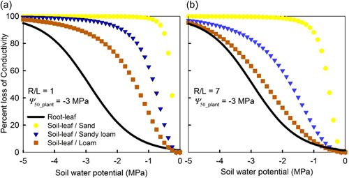
Simulated changes in the percent loss of root to leaf conductance (K _root–leaf that corresponds to whole plant xylem characterized here by a ${\psi }_{50\_\text{plant}}$, that is, a mean water potential of −3 MPa inducing 50% loss of plant conductivity) and in the percent loss of soil to leaf conductance (K _soil‐leaf, i.e., vulnerability curves of the whole soil–plant hydraulic pathway) as soil dries in different soils and with root to leaf area ratios (R/L) of 1 (a) and 7 (b). [Color figure can be viewed at wileyonlinelibrary.com]

As noted earlier, there is no advantage in having more embolism resistant plant organs in environments where soil hydraulic conductance limits water transport (Figure 5, but also see Johnson et al., 2018; Sperry et al., 1998). Indeed, reducing R/L may increase the probability of hydraulic failure as soils dry (Teskey et al., 1983) even if plants produce more embolism‐resistant xylem (Ewers et al., 2000). For instance, increasing R/L from 1 to 7 induced a shift from rhizosphere conductance to xylem loss of conductance (Figure B6). However, as R/L increased, the rhizosphere became more limiting for sandy soil, and with gradually less of an effect in less porous soils. Therefore, determining not only root area but also soil texture is essential to predict the effect of drought on plant transpiration.

Figure B6.

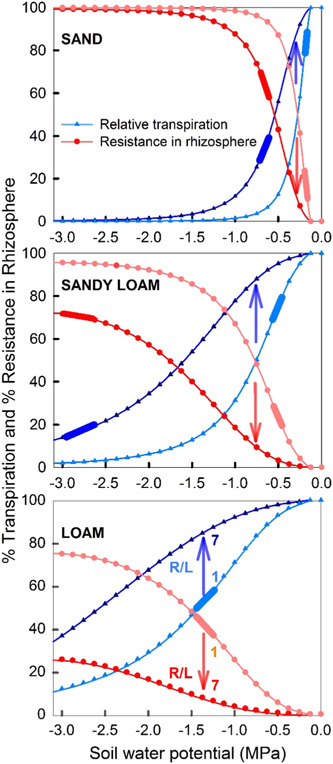
Simulated changes in relative transpiration and in the proportion of the soil to leaf hydraulic resistance (1/K _soil–leaf) located in the rhizosphere (1/K _soil–root, Figure 5) in different soils and with root area to leaf area ratios (R/L) of 1 (light blue or light red) or 7 (dark blue or dark red). Highlighted blue or red areas on each curve represent the range in critical soil water potentials (critical ${\psi }_{\mathrm{soil}}$) at which plant system experiences a transition from plant‐controlled to soil‐controlled fluxes or in other words when rhizosphere rather than xylem becomes more limiting for plant transpiration. For example, on sandy soil, critical ${\psi }_{\mathrm{soil}}$ decreased from −0.1 to −0.7 MPa when R/L increased from 1 to 7. Note that for the loam site critical ${\psi }_{\mathrm{soil}}$ at a R/L = 7 was <−10 MPa and is not represented in the figure. [Color figure can be viewed at wileyonlinelibrary.com]

In coarse soil, the loss of hydraulic conductivity occurs at water potentials less negative than plant xylem ${\psi }_{50}$ (set at −3.0 MPa; Figure B6). In sandy soil, a higher R/L was required to limit the negative impact of its high but sensitive K _soil–root on transpiration. Here, a 50% reduction in maximum transpiration occurred between −0.25 and −0.65 MPa, for a R/L of 1 and 7, respectively. At those soil water potentials, rhizosphere and xylem were nearly colimiting K _soil–leaf and thus the whole plant water transport. In contrast, in the finest soil analyzed (loam), K _soil–root did not drive K _soil–leaf and therefore the decline in transpiration became xylem‐limited and a function of xylem ${\psi }_{50}$.

These transitions in simulated soil tension are compared to predicted tipping points (${\psi }_{\mathrm{soil},\mathrm{crit}}$; see text) and reasonably agree as shown in Figure B6. Thus, ${\psi }_{\mathrm{soil},\mathrm{crit}}$, which is derived from a coordination between soil and plant hydraulics may be used as a key parameter connecting soil drying to rhizosphere contribution to water uptake the same way xylem ${\psi }_{50}$ connects plant embolism and K _root–leaf to transpiration.

These critical soil water potentials can also be converted to critical degree of saturation (i.e., fraction of soil pores filled with water) corresponding to the critical volumetric water content over the water content at saturation in the root zone ($=s_{\mathrm{crit}}$) using the soil water retention curve to yield

$${s_{\mathrm{crit}}=\left[\frac{{\psi }_{\mathrm{soil},a}}{{\psi }_{50}}\frac{K_{\mathrm{sat}}}{K_{\max }}\frac{h}{r_{\mathrm{root}}}\frac{\text{RAI}}{\log \left(\frac{r_{\mathrm{soil}}}{r_{\mathrm{root}}}\right)}\frac{\beta }{\beta +3}\right]}^{-1/(3+\beta )}.$$

This conversion of ${\psi }_{\mathrm{soil},\mathrm{crit}}$ into $s_{\mathrm{crit}}$ allows now to remotely assess and map ecosystem tipping points at larger scale using near‐surface soil moistures observed from satellites such as SMAP (https://smap.jpl.nasa.gov/).

A critique to the derivation here is that K _soil–root assumes no change in hydraulic conductivity as a function of distance to the root surface (Figure 5). When plants are exposed to severe drying, root shrinkage can create air space between roots and soil and further reduce water movement by decoupling root–soil contact (Carminati et al., 2013; Cuneo et al., 2016; North & Nobel, 1997). This decoupling was not considered in the derivation here as the goal was to assess the incipient point when maximum supply and maximum demand are in balance. Thus, the ${\psi }_{\mathrm{soil},\mathrm{crit}}$ is likely to be reached well before these drier soil conditions prevail. Notwithstanding this critique, it is worth noting that some species do develop a complex rhizosheath (i.e., a layer of adhering soil particle to the root surface bound together by mucilage root exuded either by roots or microorganisms; Price, 1911) to limit air gaps between the roots and the soil to minimize loss of hydraulic conductivity across the root–soil pathway (Basirat et al., 2019; Delhaize et al., 2015). Even though rhizosheaths are present mostly in grasses, crops and desertic plants, some woody plants have been shown to possess an enhanced rhizosheath formation (Pang et al., 2017).

7. A SURVEY OF UNDERLYING MECHANISMS GENERATING CATASTROPHES IN PLANT HYDRAULICS

To bridge the bubble‐scale to whole‐plant hydraulic failure, the mechanisms leading to the non‐linearities in the vulnerability curves across various organs and their upscaling to whole tree must be understood. Although many of these underlying mechanisms may not lead to hydraulic failure, they do underlie under‐studied pathways of water movement and structural properties in the xylem that act to ‘quarantine’ cavitation spread following embolism. These alterations to structure and function of xylem can occur in areas where catastrophic risk will become higher with climate change. To make progress on the understanding of catastrophic processes and their effects on plant hydraulics, the underlying mechanisms must first be identified and areas where urgent research is needed discussed. Here, the most relevant discoveries to plant hydraulic failure at different scales are summarized and areas where general understanding is lacking are highlighted.

7.1. Pits—structure and function

Maximum pore size in pit membranes should be the primary determinant of air‐seeding in angiosperms (Zimmermann, 1983; Tyree & Sperry, 1989) and the air‐seeding and filling of a conduit with air is another example of a catastrophe (as in the bubble expansion example, above). Network theories in which air spread within the xylem is based on maximum pit membrane pore size also proved effective in predicting the shape of vulnerability curves (Mrad et al., 2018). According to extreme value theory, selecting the maximum pore of each pit membrane and determining their probability distribution across the entire organ converges to a generalized extreme value distribution of which the Weibull function is a special case. This probability law may offer a plausible explanation why in plant vulnerability curves appear to exhibit Weibull shaped properties (Mrad et al., 2018), analogous to the way extreme mechanical failure values are modelled in engineering systems (Bebbington et al., 2007).

However, determining actual pit membrane pores sizes has been elusive. Preparation and imaging of pit membranes is difficult as they are prone to deformation, particularly during drying (Kotowska et al., 2020; Zhang et al., 2017). Recently, Kaack et al. (2021) modelled pore sizes and obtained good agreement between predicted (based on pore sizes) and measured vulnerability curves. Another interesting and potentially important property of pit membranes is their composition: more hydrophobic or hydrophilic polymers in the membrane network may serve to either increase or decrease resistance to air‐seeding and rupturing. Novel imaging technologies may be needed to elucidate the structure of pit membranes. For example, the development of new nanometre‐scale 3D X‐ray microscopy systems may be used to detect the nano‐scale pores in these membranes and their distributions throughout the membrane matrix. This will allow determining pathlengths, constrictions (Zhang et al., 2020) and tortuosity of water pathways in xylem pits. Additionally, methods that allow the determination of pit membrane chemical composition and nanomechanical properties will be important for describing both water flow through pits and air‐seeding properties (Capron et al., 2014).

The resistance due to water flow through xylem pits is comparable to the resistance of water flow through xylem conduits in both angiosperms and gymnosperms (Pittermann et al., 2006; Sperry et al., 2005; Sperry et al., 2006). However, in gymnosperms, there does seem to be slightly more resistance in pits than in the conduits themselves (Domec et al., 2006; Pittermann et al., 2006). Water flow through a regular pit field may be better approximated by the so‐called Sampson flow, which relates the flow rate through a thin perforated plate to the pressure drop across the plate (Jensen et al., 2016). In Sampson flow, the resistance depends on the inverse cube of the perforation radius instead of inverse fourth power of the pipe radius as in the Hagen–Poiseuille flow, underscoring the hydraulic significance of large pores within the pit. Sampson flow is one possible approximation when viewing the pit field as a thin sheet with multiple but well separated pores. Although Darcy's law was determined experimentally, it has since been derived from the integration of the Navier–Stokes equation for slow, viscous flow. Therefore, Darcy's law may provide another approximation when viewing water flow through the pit as a low Reynolds number porous medium. What is clear is that understanding of water flow through pit membranes is still in its embryonic state and this is an area where improvements in theory and experiments are needed urgently.

Torus‐margo pits common in coniferous species are particularly interesting due to their mechanism of sealing and isolating functional tracheids from embolized tracheids (Hacke et al., 2004; Schulte & Hacke, 2021; see Box 4). Recent work has shown that displacement of the torus requires very little pressure difference between two adjacent tracheids: somewhere between <0.1 and 0.5 Mpa is required to move the torus from its centred position (Domec et al., 2006; Zelinka et al., 2015) but more pressure may be required to completely seal the torus against the pit wall (Schulte & Hacke, 2021). More research is needed to understand the properties of torus‐margo pits and this partial list includes: the pressure differentials required for sealing in different species and organs, the nanomechanical properties such as elastic modulus of the margo (estimated as 0.012 GPa for Pinus taeda from force–displacement curves performed with an atomic force microscopy; Domec et al., unpublished data), the importance of the fit of the torus‐chamber seal (sometimes called overlap; Delzon et al., 2010) and how much of current estimates are sensitive to methodological issues (SEM, drying), the occurrence of pores in the torus (Jansen et al., 2012) and its mechanical properties, the permanence of torus aspiration (Comstock & Côté, 1968), and weakening of the margo fibres from repeated stretching (see below).

With regard to structural properties, xylem in certain species can have reductions in embolism resistance over courses of embolism and refilling (Feng et al., 2021; Hacke et al., 2001) and negative pressure cycles (Umebayashi et al., 2019). The underlying mechanism behind ‘cavitation fatigue’ is thought to be structural fatigue of the pit membrane due to stretching (Hillabrand et al., 2016; Tixier et al., 2014). This stretching is a result of pressure differentials across the pit membrane, and a progressive loss of elasticity can at some point create a bifurcation between different equilibriums thus leading to a catastrophic behaviour (Zeeman, 1978, video). For example, if an embolized conduit is adjacent to a fully functional one, the pressure in the embolized conduit will reflect atmospheric but water in the functioning conduit will be under tension thus pulling the membrane toward the functional conduit. Multiple cycles of stretching and relaxing may lead to weakened membranes that are more prone to air‐seeding. The reduction in embolism resistance due to cavitation fatigue will have hysteretic effects on plant hydraulic function and could lead to runaway cavitation (Sperry et al., 1998) and plant death.

7.2. Hydraulic network properties

Although of great interest for decades (see Zimmermann, 1983), hydraulic network topology has proven difficult to measure (but see Schenk et al., 2008; Zanne et al., 2006). Models have been developed to address the topics of the degree of vessel interconnectedness or sectoriality (Loepfe et al., 2007). More recently, Mrad et al. (2018) used pit membrane and vessel properties to develop a network model to successfully upscale to branch‐level vulnerability curves in a diffuse‐porous species. In this model, vessel element and pit resistances are determined using Hagen–Poiseuille and Sampson flow theories respectively. The model captures pertinent xylem features that allow the manifestation of the ‘rare‐pit’ hypothesis (Christman et al., 2009). Initial embolisms are introduced followed by gradual increase of bubble pressure to induce air‐seeding events similar to the air‐injection technique. The process goes on until 100% loss of conductivity occurs as shown in Figure 6 and the computed vulnerability curve is featured in Figure 7.

Figure 6.

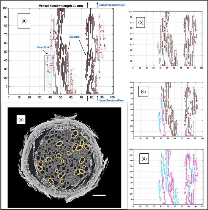
(a) Xylem model network on a 100 × 100 grid. Vertical (black) lines correspond to vessels made up of stacked vessel elements. In this case, the xylem segment is 200 mm long. Horizontal (red) lines correspond to pit membranes (simple pits in the case of angiosperms). For easier visualization of the pit membranes that have negligible thickness compared to vessel lengths, horizontal grid lines are not to scale. Some vessels conduct more xylem water than others do, and in this example, the ones located in the ‘dead end’ as represented above conduct a relatively negligible amount of water. Simulation of an air injection experiment with two initial random embolisms in each cluster (blue) leaving other vessels isolated (magenta) is represented in (b). As air pressure is increased incrementally, initial embolisms propagate and nine embolized vessels (as opposed to 4 in b) are visible in (c). Simulations continues until both clusters becomes completely disconnected and non‐conducting (d). Panel (e) shows a cross section of a Quercus root with yellow ovals indicating vessels that are connected (represented as red horizontal lines in panel (a); for more information, see Johnson et al., 2014). Scale bar represents 500 µm. [Color figure can be viewed at wileyonlinelibrary.com]

Figure 7.

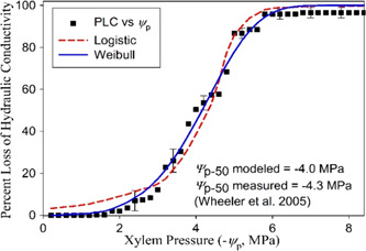
The percent loss of hydraulic conductivity (PLC) of the xylem network earlier shown (filled squares) against xylem tension. To eliminate the effect of random initial embolism locations, 40 air‐injection simulations were performed and averaged. Logistic and Weibull fits to VCs are shown for reference. Vertical bars represent variability corresponding to initial condition sensitivity. No statistically significant difference between logistic and Weibull were apparent in this case though the Weibull shape better captures the simulation outcome at low xylem pressures. The estimated xylem pressure at which ${\psi }_P$ _‐50 occurred are also compared well with measured ${\psi }_P$ _‐50 in a similar network (Wheeler et al., 2005). [Color figure can be viewed at wileyonlinelibrary.com]

Mrad et al. (2021) extended this model to test the effects of vessel connectivity and found that greater connectivity resulted in reduced embolism spread and also highlighted the large effect that vessel length has on hydraulic conductivity. Hydraulic network properties also have implications for catastrophe like behaviour. One question arising from this is ‘Would a more integrated (more vessel‐vessel connections) or a more solitary network topology be more likely to suffer runaway cavitation?’ The work of Mrad et al. (2021) suggests that there may be optimal degrees of vessel‐vessel integration to prevent catastrophic hydraulic failure.

Much work has been devoted to analysis of xylem conduit diameters and the resulting impacts on hydraulic conductivity (e.g., McCulloh et al., 2010) and their tapering from tree base to tip (Anfodillo et al., 2006; Olson et al., 2021). However, conduit length has an equally large (if not larger) effect on the overall resistance of the xylem system due to minimizing the numbers of pit crossings. Although vessel length distributions are labour intensive, future work can be directed towards understanding conduit length distributions and their effects on hydraulic transport. Undoubtedly, network topology should include coniferous and ring porous species and the impact of vasicentric tracheids (Carlquist, 1985; Percolla et al., 2021) and vessel relays (Brodersen et al., 2013) on xylem network properties.

Compared to the ‘superhighway’ of dead cells that make up the xylem, the symplastic pathways of hydraulic transport through plants have much greater resistance to water flow. These pathways occur in the leaf (parenchyma) and the root (endodermis) and are likely six–seven orders of magnitude less conductive than xylem conduits (e.g., Hammond et al., 2021). Potential other symplastic flows could be in parenchymatous tissue in the xylem (e.g., ray parenchyma) or in connecting xylem and phloem (see below). At this point, it is not known whether or not these tissues could serve as failure points for hydraulic transport through entire plants. It appears that aquaporins play a large role in transport through these tissues (Domec et al., 2021; Maurel & Prado, 2017) and if aquaporin activity was reduced to make these tissues even lower in conductivity, then they could become large bottlenecks that could result in plant tipping points for hydraulic failure. There is an undisputed need into exploring the relative conductances of these tissues and how they change with dehydration. Additional research is also needed on the effectiveness of aquaporins in water transport as tissues dehydrate.

Water flow through leaves is an exciting and developing field. Water must be transported apoplastically through the leaf venation system and may also be transported apoplastically along the cell walls of mesophyll tissue before evaporating into intercellular spaces. However, many leaves contain endodermis‐like bundle sheaths around the vascular tissue (Lersten, 1997; Liesche et al., 2021; Trueba et al., 2022) that may force water through the symplast of the bundle sheath. Further, the bundle sheath (suberized or not) exerts strong control over whole leaf hydraulic transport and aquaporins appear to be involved in water movement across the bundle sheath (Moshelion et al., 2015; Shatil‐Cohen et al., 2011). The pathways of water through leaves are complex and less well‐understood than those through xylem but new modelling and imaging developments are expanding the understanding of leaf water transport (Albuquerque et al., 2020; Trueba et al., 2022). One of the largest unknowns in symplastic transport of leaves and roots is knowledge of individual cell water transport properties and how they vary through time but also with species and in different organs.

Arguably, one of the least well‐understood water transport pathways in woody plants is the symplastic flow from phloem and inner bark through the cambial region and into the xylem (and the reverse) (Pfautsch et al., 2015; Sevanto et al., 2011). A recent study has shown that if this hydraulic transport pathway fails, this failure could represent a tipping point for tree mortality (Hammond et al., 2021; Lamacque et al., 2020; Preisler et al., 2021). In the study of Preisler et al. (2021), droughted trees that had received drought‐ending precipitation either resumed radial water transport to predrought levels and survived or did not resume radial water transport and died. The failure of radial water transport happened months before axial (sap flow) transport failed. Similarly, Lamacque et al. (2020) observed that in droughted lavender plants, once a threshold of branch diameter shrinkage had occurred, the plants could no longer rehydrate, suggesting that the phloem and cambial tissues were dead and suppressed radial water flow altogether. Radial water transport between phloem and xylem may be a new target for monitoring the likelihood of trees succumbing to mortality due to drought and drought and rewatering experiments combining sap flow and dendrometers could be used to determine these thresholds for mortality.

7.3. Spatial scales—from organ vulnerability curves to whole plant function

Organ level hydraulic function and dysfunction is now endowed with existing data on thousands of species. Branches, in particular, are well studied with over 2000 published vulnerability curves (Choat et al., 2012). However, much fewer studies have been performed on whole‐plant and plant–soil hydraulics and vulnerability to hydraulic dysfunction (Binks et al., 2022; Cai et al., 2021; McCulloh et al., 2019). This is due to the difficulty of measuring hydraulic failure in intact plants and is particularly difficult in large trees. There are ways to overcome these limitations. During drought experiments, transpiration can be measured having trees in lysimeters and water potentials can be measured with stem psychrometers (Guo et al., 2020; Williams et al., 2021) and soil psychrometers. Control plants can be destructively sampled, and vulnerability curves can be obtained from roots, trunks, branches and leaves and soil moisture release curves can be obtained using multiple methods (Jury & Horton, 2004). These types of experiments can resolve where hydraulic failure is occurring during drought and whether it is in the plant or in the soil. The one missing piece of these experiments would be fine roots: if no apparent hydraulic failure was observed in the plant or the soil then fine roots would be the most likely culprit.

In recent years, multiple technologies have been developed for remote sensing of plant water stress. Vegetation water content has been estimated using remote sensing techniques for decades (e.g., Jackson et al., 2004) and new microwave‐based methods offer deeper penetration into forest canopies than other methods and are insensitive to cloud cover (Konings et al., 2021). In fact, microwave‐based measurements of canopy relative water content were found to be the best predictor of tree mortality in a recent drought in California (Rao et al., 2019). This new development makes remote sensing a tool for monitoring and understanding forest responses to changes in climate in ways never fathomed just a decade earlier. As more new technologies for detecting water content, and potentially, hydraulic function in forests are developed, an understanding of whole‐plant–soil hydraulic systems will be even more important for interpreting what remote sensing technologies are revealing about the status of trees and how ‘early warning' signals can be derived and interpreted.

8. CONCLUSIONS

Catastrophe theory was applied to describe critical or tipping points in simplified dynamical systems representing bubble expansion, embolism spread in xylem networks, hydraulic dysfunction, and forest and tree mortality when represented by the von Bertalanffy equation. Similar framework has been successfully employed in the ecological literature but received scant attention in plant hydraulics. The framework described here established mechanistic links between the critical points and key control variables thereby uncovering generic classes of catastrophes within the xylem system. Control variables such as the size and amount of air molecules in embryonic bubbles that enter a xylem conduit are shown to result in a ‘fold’ catastrophe. When accounting for cell wall geometry and their mechanical properties to constrain the maximum bubble size transformed the aforementioned fold to a cusp catastrophe. Moving from stability of bubbles within a conduit to spread of bubbles across conduits, it was shown that competition between the ease by which cavitation spreads across xylem conduits and self‐limiting controls also lead to a fold catastrophe. The consequences of xylem hydraulics and the control variables describing these catastrophes appear to have minimal impact on the safety‐efficiency tradeoff hypothesis. The role of allometric scaling exponents on tipping points within the plant carbon balance was also analyzed and shown to result in a fold catastrophe formed by a transcritical bifurcation when the exponent is different from unity (i.e., the dynamical system must be non‐linear). These findings underscore the fact that to move this field and concept forward, connecting structure and processes that are least understood must be undertaken to uncover the nature of non‐linearities in models for the soil–plant continuum. By models of the soil–plant continuum, we mean models that assume continuous water potential from soil to leaf along the chain of interconnected water molecules. These processes include xylem network properties, pit structure and function, belowground hydraulic processes, and whole‐plant hydraulics. Additionally, a greater understanding of under what conditions and processes plant transpiration transitions from plant‐controlled to soil‐controlled will move the field forward. Because near‐surface soil moisture across the globe from remote sensing platforms may be in reach within the foreseeable future, knowledge of soil moisture impacts on the entire soil to leaf hydraulic pathway are becoming ever more important (i.e., $s_{\mathit{crit}})$. Strengthening the scientific knowledge around these key aspects of plant hydraulics will enable predictions of tipping points for plant hydraulic failure and mortality when both exogenous and endogenous conditions are gradually altered.

CONFLICTS OF INTERESTS

The authors declare no conflicts of interest.

Johnson, D. M. , Katul, G. & Domec, J.‐C. (2022) Catastrophic hydraulic failure and tipping points in plants. Plant, Cell & Environment, 45, 2231–2266. 10.1111/pce.14327

DATA AVAILABILITY STATEMENT

All data are available from the corresponding author upon reasonable request.

REFERENCES

- Adams, H.D. , Zeppel, M.J. , Anderegg, W.R. , Hartmann, H. , Landhäusser, S.M. , Tissue, D.T. et al. (2017) A multi‐species synthesis of physiological mechanisms in drought‐induced tree mortality. Nature Ecology and Evolution, 1, 1285–1291. [DOI] [PubMed] [Google Scholar]
- Albuquerque, C. , Scoffoni, C. , Brodersen, C.R. , Buckley, T.N. , Sack, L. & McElrone, A.J. (2020) Coordinated decline of leaf hydraulic and stomatal conductances under drought is not linked to leaf xylem embolism for different grapevine cultivars. Journal of Experimental Botany, 71, 7286–7300. [DOI] [PubMed] [Google Scholar]
- Allen, C.D. , Breshears, D.D. & McDowell, N.G. (2015) On underestimation of global vulnerability to tree mortality and forest die‐off from hotter drought in the Anthropocene. Ecosphere, 6, 1–55. [Google Scholar]
- Allen, C.D. , Macalady, A.K. , Chenchouni, H. , Bachelet, D. , McDowell, N. , Vennetier, M. et al. (2010) A global overview of drought and heat‐induced tree mortality reveals emerging climate change risks for forests. Forest Ecology and Management, 259, 660–684. [Google Scholar]
- Anfodillo, T. , Carraro, V. , Carrer, M. , Fior, C. & Rossi, S. (2006) Convergent tapering of xylem conduits in different woody species. New Phytologist, 169, 279–290. [DOI] [PubMed] [Google Scholar]
- Basirat, M. , Mousavi, S.M. , Abbaszadeh, S. & Zarebanadkouki, M. (2019) The rhizosheath: a potential root trait helping plants to tolerate drought stress. Plant Soil, 445, 565–575. [Google Scholar]
- Bebbington, M. , Lai, C.D. & Zitikis, R. (2007). A flexible weibull extension. Reliability Engineering & System Safety, 92(6), 719–726. [Google Scholar]
- Bertolino, L.T. , Caine, R.S. & Gray, J.E. (2019) Impact of stomatal density and morphology on water‐use efficiency in a changing world. Frontiers in Plant Science, 10, 225. [DOI] [PMC free article] [PubMed] [Google Scholar]
- Binks, O. , Cernusak, L.A. , Liddell, M. , Bradford, M. , Coughlin, I. , Carle, H. et al. (2022) Forest system hydraulic conductance: partitioning tree and soil components. New Phytologist, 233, 1667–1681. [DOI] [PubMed] [Google Scholar]
- Boulton, C.A. , Lenton, T.M. & Boers, N. (2022) Pronounced loss of Amazon rainforest resilience since the early 2000s. Nature Climate Change, 12, 271–278. 10.1038/s41558-022-01287-8 [DOI] [Google Scholar]
- Briggs, L.J. (1950) Limiting negative pressure of water. Journal of Applied Physics, 21, 721–722. [Google Scholar]
- Brodersen, C.R. , Choat, B. , Chatelet, D.S. , Shackel, K.A. , Matthews, M.A. & McElrone, A.J. (2013) Xylem vessel relays contribute to radial connectivity in grapevine stems (Vitis vinifera and V. arizonica; Vitaceae). American Journal of Botany, 100, 314–321. [DOI] [PubMed] [Google Scholar]
- Brodersen, C.R. , Knipfer, T. & McElrone, A.J. (2018) In vivo visualization of the final stages of xylem vessel refilling in grapevine (Vitis vinifera) stems. New Phytologist, 217, 117–126. [DOI] [PubMed] [Google Scholar]
- Brooks, R.H. & Corey, A.T. (1964) Hydraulic properties of porous media and their relation to drainage design. Transactions of the ASAE, 7, 26–28. [Google Scholar]
- Cai, G. , Carminati, A. , Abdalla, M. & Ahmed, M.A. (2021) Soil textures rather than root hairs dominate water uptake and soil–plant hydraulics under drought. Plant Physiology, 187, 858–872. [DOI] [PMC free article] [PubMed] [Google Scholar]
- Campbell, G.S. (1985) Soil Physics with Basic; Transport Models or Soil‐Plant Systems. Amsterdam: Elsevier Science Publishers. [Google Scholar]
- Capron, M. , Tordjeman, P. , Charru, F. , Badel, E. & Cochard, H. (2014) Gas flow in plant microfluidic networks controlled by capillary valves. Physical Review E, 89, 033019. [DOI] [PubMed] [Google Scholar]
- Carlquist, S. (1985) Vasicentric tracheids as a drought survival mechanism in the woody flora of southern California and similar regions; review of vasicentric tracheids. Aliso: A Journal of Systematic and Evolutionary Botany, 11, 37–68. [Google Scholar]
- Carminati, A. & Javaux, M. (2020) Soil rather than xylem vulnerability controls stomatal response to drought. Trends in Plant Science, 25, 868–880. [DOI] [PubMed] [Google Scholar]
- Carminati, A. , Vetterlein, D. , Koebernick, N. , Blaser, S. , Weller, U. & Vogel, H.J. (2013) Do roots mind the gap? Plant Soil, 367, 651–661. [Google Scholar]
- Casper, B.B. & Jackson, R.B. (1997) Plant competition underground. Annual Review of Ecology and Systematics, 28, 545–570. [Google Scholar]
- Chaumont, F. & Tyerman, S.D. (2014) Aquaporins: highly regulated channels controlling plant water relations. Plant Physiology, 164, 1600–1618. [DOI] [PMC free article] [PubMed] [Google Scholar]
- Choat, B. , Jansen, S. , Brodribb, T.J. , Cochard, H. , Delzon, S. , Bhaskar, R. et al. (2012) Global convergence in the vulnerability of forests to drought. Nature, 491, 752–755. [DOI] [PubMed] [Google Scholar]
- Christman, M.A. , Sperry, J.S. & Adler, F.R. (2009) Testing the ‘rare pit’ hypothesis for xylem cavitation resistance in three species of Acer. New Phytologist, 182, 664–674. [DOI] [PubMed] [Google Scholar]
- Cochard, H. , Herbette, S. , Barigah, T. , Badel, E. , Ennajeh, M. & Vilagrosa, A. (2010) Does sample length influence the shape of xylem embolism vulnerability curves? A test with the Cavitron spinning technique. Plant, Cell & Environment, 33, 1543–1552. [DOI] [PubMed] [Google Scholar]
- Comstock, G.L. & Côté, W.A. (1968) Factors affecting permeability and pit aspiration in coniferous sapwood. Wood Science and Technology, 2, 279–291. [Google Scholar]
- Cuneo, I. , Knipfer, T. , Brodersen, C. & McElrone, A. (2016) Mechanical failure of fine root cortical cells initiates plant hydraulic declined during drought. Plant Physiology, 172, 1669–1678. [DOI] [PMC free article] [PubMed] [Google Scholar]
- Darwin, F. , Vines, S.H. , Joly, J. & FitzGerald, G.F. (1896) Report of a discussion on the ascent of water in trees. Annals of Botany, 10, 630–661. [Google Scholar]
- Delhaize, E. , Rathjen, T.M. & Cavanagh, C.R. (2015) The genetics of rhizosheath size in a multiparent mapping population of wheat. Journal of Experimental Botany, 66, 4527–4536. [DOI] [PMC free article] [PubMed] [Google Scholar]
- Delzon, S. , Douthe, C. , Sala, A. & Cochard, H. (2010) Mechanism of water‐stress induced cavitation in conifers: bordered pit structure and function support the hypothesis of seal capillary‐seeding. Plant Cell Environment, 33, 2101–2111. [DOI] [PMC free article] [PubMed] [Google Scholar]
- Dietze, M.C. & Moorcroft, P.R. (2011) Tree mortality in the eastern and central United States: patterns and drivers. Global Change Biology, 17, 3312–3326. [Google Scholar]
- Dittmer, H.J. (1949) Root hair variations in plant species. American Journal of Botany, 36, 152–155. [Google Scholar]
- Dixon, H.H. , & Joly, J. (1894). On the ascent of sap. Proceedings of the Royal Society of London, 57, 3–5. [Google Scholar]
- Domec, J.C. & Gartner, B.L. (2001) Cavitation and water storage capacity in bole xylem segments of mature and young Douglas‐fir trees. Trees, 15, 204–214. [Google Scholar]
- Domec, J.C. , King, J.S. , Carmichael, M.J. , Overby, A.T. , Wortemann, R.R. , Smith, W.K. et al. (2021) Root water gates and not changes in root structure provide new insights into plant physiological responses to drought, flooding and salinity. Journal of Experimental Botany, 72, 4489–4501. [DOI] [PubMed] [Google Scholar]
- Domec, J.C. , Lachenbruch, B.L. & Meinzer, F.C. (2006) Bordered pit structure and function determine spatial patterns of air‐seeding thresholds in xylem of Douglas‐fir (Pseudostuga menziesii; Pinaceae) trees. American Journal of Botany, 93, 1588–1600. [DOI] [PubMed] [Google Scholar]
- Domec, J.C. , Noormets, A. , King, J.S. , Sun, G. , McNulty, S.G. , Gavazzi, M.J. et al. (2009) Decoupling the influence of leaf and root hydraulic conductances on stomatal conductance and its sensitivity to vapour pressure deficit as soil dries in a drained loblolly pine plantation. Plant Cell Environment, 32, 980–991. [DOI] [PubMed] [Google Scholar]
- Domec, J.C. , Ogée, J. , Noormets, A. , Jouangy, J. , Gavazzi, M. , Treasure, E. et al. (2012) Interactive effects of nocturnal transpiration and climate change on the root hydraulic redistribution and carbon and water budgets of Southern US pine plantations. Tree Physiology, 32, 707–723. [DOI] [PubMed] [Google Scholar]
- Doussan, C. , Vercambr, G. & Page, L. (1998) Modelling of the hydraulic architecture of root systems: an integrated approach to water absorption—distribution of axial and radial conductances in maize. Annals of Botany, 81, 225–232. [Google Scholar]
- Draye, X. , Kim, Y. , Lobet, G. & Javaux, M. (2010) Model‐assisted integration of physiological and environmental constraints affecting the dynamic and spatial patterns of root water uptake from soils. Journal of Experimental Botany, 61, 2145–2155. [DOI] [PubMed] [Google Scholar]
- Duan, C. , Karnik, R. , Lu, M.C. & Majumdar, A. (2012) Evaporation‐induced cavitation in nanofluidic channels. Proceedings of the National Academy of Sciences, 109, 3688–3693. [DOI] [PMC free article] [PubMed] [Google Scholar]
- Dute, R.R. (2015) Development, structure, and function of torus‐margo pits in conifers, Ginkgo and dicots. In: Hacke, U.G. , ed. Functional and ecological xylem anatomy. Cham, Switzerland: Springer International. pp. 77–102. [Google Scholar]
- Ehlert, C. , Maurel, C. , Tardieu, F. & Simonneau, T. (2009) Aquaporin‐mediated reduction in maize root hydraulic conductivity impacts cell turgor and leaf elongation even without changing transpiration. Plant Physiology, 150, 1093–1104. [DOI] [PMC free article] [PubMed] [Google Scholar]
- Ewers, B.E. , Oren, R. & Sperry, J.S. (2000) Influence of nutrient versus water supply on hydraulic architecture and water balance in Pinus taeda . Plant Cell Environment, 23, 1055–1066. [Google Scholar]
- Feng, F. , Losso, A. , Tyree, M. , Zhang, S. & Mayr, S. (2021) Cavitation fatigue in conifers: a study on eight European species. Plant Physiology, 186, 1580–1590. [DOI] [PMC free article] [PubMed] [Google Scholar]
- Givnish, T.J. & Vermeij, G.J. (1976) Sizes and shapes of liane leaves. The American Naturalist, 110, 743–778. [Google Scholar]
- Guo, J.S. , Hultine, K.R. , Koch, G.W. , Kropp, H. & Ogle, K. (2020) Temporal shifts in iso/anisohydry revealed from daily observations of plant water potential in a dominant desert shrub. New Phytologist, 225, 713–726. [DOI] [PubMed] [Google Scholar]
- Guswa, A.J. (2008) The influence of climate on root depth: A carbon cost‐benefit analysis. Water Resources Research, 44, W02427. [Google Scholar]
- Hacke, U.G. , Sperry, J.S. , Ewers, B.E. , Ellsworth, D.S. , Schäfer, K.V.R. & Oren, R. (2000) Influence of soil porosity on water use in Pinus taeda . Oecologia, 124, 495–505. [DOI] [PubMed] [Google Scholar]
- Hacke, U.G. , Sperry, J.S. & Pittermann, J. (2004) Analysis of circular bordered pit function II. Gymnosperm tracheids with torus‐margo pit membranes. American Journal of Botany, 91, 386–400. [DOI] [PubMed] [Google Scholar]
- Hacke, U.G. , Stiller, V. , Sperry, J.S. , Pittermann, J. & McCulloh, K.A. (2001) Cavitation fatigue. Embolism and refilling cycles can weaken the cavitation resistance of xylem. Plant Physiology, 125, 779–786. [DOI] [PMC free article] [PubMed] [Google Scholar]
- Hammond, W.M. , Yu, K. , Wilson, L.A. , Will, R.E. , Anderegg, W.R. & Adams, H.D. (2019) Dead or dying? Quantifying the point of no return from hydraulic failure in drought‐induced tree mortality. New Phytologist, 223, 1834–1843. [DOI] [PMC free article] [PubMed] [Google Scholar]
- Hammond, W.M. (2020) A matter of life and death: alternative stable states in trees, from xylem to ecosystems. Frontiers in Forests and Global Change, 3 . 10.3389/ffgc.2020.560409 [DOI] [Google Scholar]
- Hammond, W.M. , Johnson, D.M. & Meinzer, F.C. (2021) A thin line between life and death: radial sap flux failure signals trajectory to tree mortality. Plant Cell Environment, 44, 1311–1314. [DOI] [PubMed] [Google Scholar]
- Hethcote, H. (2000) The mathematics of infectious diseases. SIAM Review, 42, 599–653. [Google Scholar]
- Hillabrand, R.M. , Hacke, U.G. & Lieffers, V.J. (2016) Drought‐induced xylem pit membrane damage in aspen and balsam poplar. Plant Cell Environment, 39, 2210–2220. [DOI] [PubMed] [Google Scholar]
- Holbrook, N.M. & Zwieniecki, M.A. (1999) Embolism repair and xylem tension. Do we need a miracle? Plant Physiology, 120, 7–10. [DOI] [PMC free article] [PubMed] [Google Scholar]
- Hölttä, T. , Vesala, T. & Nikinmaa, E. (2007) A model of bubble growth leading to xylem conduit embolism. Journal of Theoretical Biology, 249, 111–123. [DOI] [PubMed] [Google Scholar]
- Hsiao, T.C. (1973) Plant responses to water stress. Annual Review of Plant Physiology, 24, 519–570. [Google Scholar]
- Huang, C.W. , Domec, J.C. , Ward, E.J. , Duman, T. , Manoli, G. , Parolari, A.J. et al. (2017) The effect of plant water storage on water fluxes within the coupled soil–plant system. New Phytologist, 213, 1093–1106. [DOI] [PubMed] [Google Scholar]
- Hunt, A.G. (2005) Basic transport properties in natural porous media. Complexity, 10(1), 22–37. [Google Scholar]
- Israelachvili, J.N. & Pashley, R.M. (1983) Molecular layering of water at surfaces and origin of repulsive hydration forces. Nature, 306, 249–250. [Google Scholar]
- Jackson, T.J. , Chen, D. , Cosh, M. , Li, F. , Anderson, M. , Walthall, C. et al. (2004) Vegetation water content mapping using Landsat data derived normalized difference water index for corn and soybeans. Remote Sensing of Environment, 92, 475–482. [Google Scholar]
- Jansen, S. , Lamy, J.B. , Burlett, R. , Cochard, H. , Gasson, P. & Delzon, S. (2012) Plasmodesmatal pores in the torus of bordered pit membranes affect cavitation resistance of conifer xylem. Plant Cell Environment, 35, 1109–1120. [DOI] [PubMed] [Google Scholar]
- Jensen, K.H. , Berg‐Sørensen, K. , Bruus, H. , Holbrook, N.M. , Liesche, J. , Schulz, A. et al. (2016) Sap flow and sugar transport in plants. Reviews of Modern Physics, 88, 035007. [Google Scholar]
- Johnson, D.M. , Brodersen, C.R. , Reed, M. , Domec, J.C. & Jackson, R.B. (2014) Contrasting hydraulic architecture and function in deep and shallow roots of two co‐occurring tree species from an arid habitat. Annals of Botany, 113, 617–627. [DOI] [PMC free article] [PubMed] [Google Scholar]
- Johnson, D.M. , Domec, J.C. , Berry, Z.C. , Schwantes, A.M. , McCulloh, K.A. , Woodruff, D.R. et al. (2018) Co‐occurring woody species have diverse hydraulic strategies and mortality rates during an extreme drought. Plant Cell Environment, 41, 576–588. [DOI] [PubMed] [Google Scholar]
- Johnson, D.M. , Wortemann, R. , McCulloh, K.A. , Jordan‐Meille, L. , Ward, E. , Warren, J.M. et al. (2016) A test of the hydraulic vulnerability segmentation hypothesis in angiosperm and conifer tree species. Tree physiology, 36, 983–993. [DOI] [PubMed] [Google Scholar]
- Jury, W.A. & Horton, R. (2004) Soil Physics. New York, NY: John Wiley & Sons. [Google Scholar]
- Kaack, L. , Weber, M. , Isasa, E. , Karimi, Z. , Li, S. , Pereira, L. et al. (2021) Pore constrictions in intervessel pit membranes provide a mechanistic explanation for xylem embolism resistance in angiosperms. New Phytologist (online early), 230, 1829–1843. [DOI] [PubMed] [Google Scholar]
- Kaack, L.H. & Katul, G.G. (2013) Fifty years to prove Malthus right. Proceedings of the National Academy of Sciences, 110(11), 4161–4162. [DOI] [PMC free article] [PubMed] [Google Scholar]
- Katul, G. , Manzoni, S. , Palmroth, S. & Oren, R. (2010) A stomatal optimization theory to describe the effects of atmospheric CO2 on leaf photosynthesis and transpiration. Annals of Botany, 105, 431–442. [DOI] [PMC free article] [PubMed] [Google Scholar]
- Katul, G.G. , Mrad, A. , Bonetti, S. , Manoli, G. & Parolari, A.J. (2020) Global convergence of COVID‐19 basic reproduction number and estimation from early‐time SIR dynamics. PLoS One, 15(9), e0239800. [DOI] [PMC free article] [PubMed] [Google Scholar]
- Kermack, W. & McKendrick, A. (1927) A contribution to the mathematical theory of epidemics. Proceedings of the Royal Society of London Series A‐Containing Papers of a Mathematical and Physical Character, 15, 700–721. [Google Scholar]
- Konings, A.G. , Katul, G.G. & Porporato, A. (2010) The rainfall‐no rainfall transition in a coupled land‐convective atmosphere system. Geophysical Research Letters, 37, L14401. [Google Scholar]
- Konings, A.G. , Saatchi, S.S. , Frankenberg, C. , Keller, M. , Leshyk, V. , Anderegg, W.R. et al. (2021) Detecting forest response to droughts with global observations of vegetation water content. Global Change Biology, 27, 6005–6024. [DOI] [PMC free article] [PubMed] [Google Scholar]
- Konrad, W. , Katul, G. , Roth‐Nebelsick, A. & Jensen, K.H. (2019) Xylem functioning, dysfunction and repair: a physical perspective and implications for phloem transport. Tree Physiology, 39, 243–261. [DOI] [PubMed] [Google Scholar]
- Konrad, W. & Roth‐Nebelsick, A. (2003) The dynamics of gas bubbles in conduits of vascular plants and implications for embolism repair. Journal of Theoretical Biology, 224, 43–61. [DOI] [PubMed] [Google Scholar]
- Konrad, W. & Roth‐Nebelsick, A. (2005) The significance of pit shape for hydraulic isolation of embolized conduits of vascular plants during novel refilling. Journal of Biological Physics, 31, 57–71. [DOI] [PMC free article] [PubMed] [Google Scholar]
- Konrad, W. & Roth‐Nebelsick, A. (2006) Embolism formation and repair in vascular plants: the role of cell wall mechanics. In Proceedings of the 5th Plant Biomechanics Conference, Editor: Lennart Salmn, Stockholm (p. 417422).
- Konrad, W. & Roth‐Nebelsick, A. (2009) The influence of the wall contact angle on gas bubble behaviour in xylem conduits under tension and possible consequences for embolism. In Proceedings of the Sixth Plant Biomechanics Conference. Institut für Angewandte Physik, Vienna (pp. 32–39).
- Körner, C. (2019) No need for pipes when the well is dry—a comment on hydraulic failure in trees. Tree Physiology, 39, 695–700. [DOI] [PubMed] [Google Scholar]
- Kotowska, M.M. , Thom, R. , Zhang, Y. , Schenk, H.J. & Jansen, S. (2020) Within‐tree variability and sample storage effects of bordered pit membranes in xylem of Acer pseudoplatanus. Trees, 34, 61–71. [Google Scholar]
- Lamacque, L. , Charrier, G. , Farnese, F.D.S. , Lemaire, B. , Améglio, T. & Herbette, S. (2020) Drought‐induced mortality: branch diameter variation reveals a point of no recovery in lavender species. Plant Physiology, 183, 1638–1649. [DOI] [PMC free article] [PubMed] [Google Scholar]
- Landau, L.D. & Lifshitz, E.M. (1987) Theoretical Physics, vol. 6, Fluid Mechanics 557 pp, 2nd ed. Oxford, UK: Pergamon Press. [Google Scholar]
- Lersten, N.R. (1997) Occurrence of endodermis with a casparian strip in stem and leaf. The Botanical Review, 63, 265–272. [Google Scholar]
- Liesche, J. , Vincent, C. , Han, X. , Zwieniecki, M. , Schulz, A. , Gao, C. et al. (2021) The mechanism of sugar export from long conifer needles. New Phytologist, 230, 1911–1924. [DOI] [PubMed] [Google Scholar]
- Liu, Y. , Kumar, M. , Katul, G.G. , Feng, X. & Konings, A.G. (2020) Plant hydraulics accentuates the effect of atmospheric moisture stress on transpiration. Nature Climate Change, 10, 691–695. [Google Scholar]
- Liu, Y. , Kumar, M. , Katul, G.G. & Porporato, A. (2019) Reduced resilience as an early warning signal of forest mortality. Nature Climate Change, 9, 880–885. [Google Scholar]
- Loepfe, L. , Martinez‐Vilalta, J. , Piñol, J. & Mencuccini, M. (2007) The relevance of xylem network structure for plant hydraulic efficiency and safety. Journal of Theoretical Biology, 247, 788–803. [DOI] [PubMed] [Google Scholar]
- Ludwig, D. , Jones, D.D. & Holling, C.S. (1978) Qualitative analysis of insect outbreak systems: the spruce budworm and forest. The Journal of Animal Ecology, 47, 315–332. [Google Scholar]
- Martin‐StPaul, N.K. , Longepierre, D. , Huc, R. , Delzon, S. , Burlett, R. , Joffre, R. et al. (2014) How reliable are methods to assess xylem vulnerability to cavitation? The issue of ‘open vessel’ artifact in oaks. Tree Physiology, 34, 894–905. [DOI] [PubMed] [Google Scholar]
- Manoli, G. , Huang, C.W. , Bonetti, S. , Domec, J.C. , Marani, M. & Katul, G. (2017) Competition for light and water in a coupled soil‐plant system. Advances in Water Resources, 108, 216–230. [Google Scholar]
- Manzoni, S. , Katul, G. & Porporato, A. (2014) A dynamical system perspective on plant hydraulic failure. Water Resources Research, 50, 5170–5183. [Google Scholar]
- Manzoni, S. , Vico, G. , Katul, G. , Palmroth, S. , Jackson, R.B. & Porporato, A. (2013) Hydraulic limits on maximum plant transpiration and the emergence of the safety‐efficiency trade‐off. New Phytologist, 198, 169–178. [DOI] [PubMed] [Google Scholar]
- Maurel, C. & Prado, K. (2017) Aquaporins and leaf water relations, Plant aquaporins. Springer, pp. 155–165. [Google Scholar]
- McCulloh, K. , Sperry, J.S. , Lachenbruch, B. , Meinzer, F.C. , Reich, P.B. & Voelker, S. (2010) Moving water well: comparing hydraulic efficiency in twigs and trunks of coniferous, ring‐porous, and diffuse‐porous saplings from temperate and tropical forests. New Phytologist, 186, 439–450. [DOI] [PubMed] [Google Scholar]
- McCulloh, K.A. , Domec, J.C. , Johnson, D.M. , Smith, D.D. & Meinzer, F.C. (2019) A dynamic yet vulnerable pipeline: integration and coordination of hydraulic traits across whole plants. Plant Cell Environment, 42, 2789–2807. [DOI] [PubMed] [Google Scholar]
- McCully, M.E. (1999) Roots in soil: unearthing the complexities of roots and their rhizospheres. Annual Review of Plant Physiology and Plant Molecular Biology, 50, 695–718. [DOI] [PubMed] [Google Scholar]
- Meinzer, F.C. , Johnson, D.M. , Lachenbruch, B. , McCulloh, K.A. & Woodruff, D.R. (2009) Xylem hydraulic safety margins in woody plants: coordination of stomatal control of xylem tension with hydraulic capacitance. Functional Ecology, 23, 922–930. [Google Scholar]
- Meyra, A.G. , Zarragoicoechea, G.J. & Kuz, V.A. (2011) A similarity law in botanic. The case of hydraulic conductivity of trees. The European Physical Journal D, 62, 19–23. [Google Scholar]
- Millburn, J.A. & Johnson, R.P.C. (1966) The conduction of sap. I. Detection of vibrations produced by sap cavitation in Ricinus xylem. Planta, 69, 43–52. [DOI] [PubMed] [Google Scholar]
- Mooney, H.A. (1972) The carbon balance of plants. Annual Review of Ecology and Systematics, 3, 315–346. [Google Scholar]
- Moshelion, M. , Halperin, O. , Wallach, R. , Oren, R. & Way, D.A. (2015) Role of aquaporins in determining transpiration and photosynthesis in water‐stressed plants: crop water‐use efficiency, growth and yield. Plant Cell Environment, 38, 1785–1793. [DOI] [PubMed] [Google Scholar]
- Mrad, A. , Domec, J.C. , Huang, C.W. , Lens, F. & Katul, G. (2018) A network model links wood anatomy to xylem tissue hydraulic behaviour and vulnerability to cavitation. Plant Cell Environment, 41, 2718–2730. [DOI] [PubMed] [Google Scholar]
- Mrad, A. , Johnson, D.M. , Love, D.M. & Domec, J.C. (2021) The roles of conduit redundancy and connectivity in xylem hydraulic functions. New Phytologist, 231, 996–1007. [DOI] [PubMed] [Google Scholar]
- Mrad, A. , Manzoni, S. , Oren, R. , Vico, G. , Lindh, M. & Katul, G. (2020) Recovering the metabolic, self‐thinning, and constant final yield rules in mono‐specific stands. Frontiers in Forests and Global Change, 3, 62. [Google Scholar]
- Mrad, A. , Sevanto, S. , Domec, J.C. , Liu, Y. , Nakad, M. & Katul, G. (2019) A dynamic optimality principle for water use strategies explains isohydric to anisohydric plant responses to drought. Frontiers in Forests and Global Change, 2, 49. [Google Scholar]
- Nobel, P.S. & Cui, M. (1992) Hydraulic conductances of the soil, the root‐sol air gap, and the root: changes for desert succulents in drying soil. Journal of Experimental Botany, 43, 319–326. [Google Scholar]
- North, G.B. & Nobel, P.S. (1997) Drought‐induced changes in soil contact and hydraulic conductivity for roots of Opuntia ficus‐indica with and without rhizosheaths. Plant and Soil, 191, 249–258. [Google Scholar]
- Novick, K.A. , Katul, G.G. , McCarthy, H.R. & Oren, R. (2012) Increased resin flow in mature pine trees growing under elevated CO2 and moderate soil fertility. Tree Physiology, 32, 752–763. [DOI] [PubMed] [Google Scholar]
- Oertli, J.J. (1971) The stability of water under tension in the xylem. Zeitschrift PJlanzen Physiologie, 65, 195–209. [Google Scholar]
- Ogle, K. , Barber, J.J. , Willson, C. & Thompson, B. (2009) Hierarchical statistical modeling of xylem vulnerability to cavitation. New Phytologist, 182, 541–554. [DOI] [PubMed] [Google Scholar]
- Olson, M.E. , Anfodillo, T. , Gleason, S.M. & McCulloh, K.A. (2021) Tip‐to‐base xylem conduit widening as an adaptation: causes, consequences, and empirical priorities. New Phytologist, 229, 1877–1893. [DOI] [PubMed] [Google Scholar]
- Pammenter, N.W. & Vander Willigen, C. (1998) A mathematical and statistical analysis of the curves illustrating vulnerability of xylem to cavitation. Tree Physiology, 18, 589–593. [DOI] [PubMed] [Google Scholar]
- Pang, J. , Ryan, M.H. , Siddique, K.H. & Simpson, R.J. (2017) Unwrapping the rhizosheath. Plant and Soil, 418, 129–139. [Google Scholar]
- Parolari, A.J. , Katul, G.G. & Porporato, A. (2014) An ecohydrological perspective on drought‐induced forest mortality. Journal of Geophysical Research: Biogeosciences, 119, 965–981. [Google Scholar]
- Parolari, A.J. , Katul, G.G. & Porporato, A. (2015) The doomsday equation and 50 years beyond: new perspectives on the human‐water system. Wiley Interdisciplinary Reviews: Water, 2, 407–414. [Google Scholar]
- Passioura, J.B. (1988) Water transport in and to roots. Annual Reviews in Plant Physiology, 39, 245–265. [Google Scholar]
- Percolla, M.I. , Fickle, J.C. , Rodríguez‐Zaccaro, F.D. , Pratt, R.B. & Jacobsen, A.L. (2021) Hydraulic function and conduit structure in the xylem of five oak species. IAWA Journal, 43, 279–298. [Google Scholar]
- Perkins, S.J. (1986) Protein volumes and hydration effects: the calculations of partial specific volumes, neutron scattering matchpoints and 280‐nm absorption coefficients for proteins and glycoproteins from amino acid sequences. European Journal of Biochemistry, 157, 169–180. [DOI] [PubMed] [Google Scholar]
- Perry, D.A. (1984) A model of physiological and allometric factors in the self‐thinning curve. Journal of Theoretical Biology, 106, 383–401. [Google Scholar]
- Pfautsch, S. , Renard, J. , Tjoelker, M.G. & Salih, A. (2015) Phloem as capacitor: radial transfer of water into xylem of tree stems occurs via symplastic transport in ray parenchyma. Plant Physiology, 167, 963–971. [DOI] [PMC free article] [PubMed] [Google Scholar]
- Pittermann, J. , Sperry, J.S. , Hacke, U.G. , Wheeler, J.K. & Sikkema, E.H. (2006) Inter‐tracheid pitting and the hydraulic efficiency of conifer wood: the role of tracheid allometry and cavitation protection. American Journal of Botany, 93, 1265–1273. [DOI] [PubMed] [Google Scholar]
- Plesset, M.S. & Prosperetti, A. (1977) Bubble dynamics and cavitation. Annual Review of Fluid Mechanics, 9(1), 145–185. [Google Scholar]
- Preisler, Y. , Tatarinov, F. , Grünzweig, J.M. & Yakir, D. (2021) Seeking the “point of no return” in the sequence of events leading to mortality of mature trees. Plant Cell Environment, 44, 1315–1328. [DOI] [PubMed] [Google Scholar]
- Price, S.R. (1911) The roots of some north African desert‐grasses. New Phytologist, 10, 328–340. [Google Scholar]
- Rao, K. , Anderegg, W.R. , Sala, A. , Martínez‐Vilalta, J. & Konings, A.G. (2019) Satellite‐based vegetation optical depth as an indicator of drought‐driven tree mortality. Remote Sensing of Environment, 227, 125–136. [Google Scholar]
- Roth‑Nebelsick, A. (2019) It's contagious: calculation and analysis of xylem vulnerability to embolism by a mechanistic approach based on epidemic modeling. Trees, 33, 1519–1533. [Google Scholar]
- Rowland, L. , da Costa, A.C.L. , Galbraith, D.R. , Oliveira, R.S. , Binks, O.J. , Oliveira, A.A.R. et al. (2015) Death from drought in tropical forests is triggered by hydraulics not carbon starvation. Nature, 528, 119–122. [DOI] [PubMed] [Google Scholar]
- Salmon, Y. , Dietrich, L. , Sevanto, S. , Hölttä, T. , Dannoura, M. & Epron, D. (2019) Drought impacts on tree phloem: from cell‐level responses to ecological significance. Tree Physiology, 39, 173–191. [DOI] [PubMed] [Google Scholar]
- Scheffer, M. , Carpenter, S. , Foley, J.A. , Folke, C. & Walker, B. (2001) Catastrophic shifts in ecosystems. Nature, 413, 591–596. [DOI] [PubMed] [Google Scholar]
- Scheffer, M. & Carpenter, S.R. (2003) Catastrophic regime shifts in ecosystems: linking theory to observation. Trends in Ecology & Evolution, 18, 648–656. [Google Scholar]
- Schenk, H.J. , Espino, S. , Goedhart, C.M. , Nordenstahl, M. , Cabrera, H.I.M. & Jones, C.S. (2008) Hydraulic integration and shrub growth form linked across continental aridity gradients. Proceedings of the National Academy of Sciences of the United States of America, 105, 11248–11253. [DOI] [PMC free article] [PubMed] [Google Scholar]
- Schulte, P.J. & Hacke, U.G. (2021) Solid mechanics of the torus–margo in conifer intertracheid bordered pits. New Phytologist, 229, 1431–1439. [DOI] [PubMed] [Google Scholar]
- Szalewicz, K. (2003) Hydrogen Bond. In: Meyers, R.A. Encyclopedia of Physical Science and Technology, Third Ed. Academic Press, pp. 505–538. [Google Scholar]
- Sevanto, S. , Hölttä, T. & Holbrook, N.M. (2011) Effects of the hydraulic coupling between xylem and phloem on diurnal phloem diameter variation. Plant Cell Environment, 34, 690–703. [DOI] [PubMed] [Google Scholar]
- Sevanto, S. (2014) Phloem transport and drought. Journal of Experimental Botany, 65(7), 1751–1759. [DOI] [PubMed] [Google Scholar]
- Sevanto, S. , Mcdowell, N.G. , Dickman, L.T. , Pangle, R. & Pockman, W.T. (2014) How do trees die? A test of the hydraulic failure and carbon starvation hypotheses. Plant Cell Environment, 37, 153–161. [DOI] [PMC free article] [PubMed] [Google Scholar]
- Shatil‐Cohen, A. , Attia, Z. & Moshelion, M. (2011) Bundle‐sheath cell regulation of xylem‐mesophyll water transport via aquaporins under drought stress: a target of xylem‐borne ABA? The Plant Journal, 67, 72–80. [DOI] [PubMed] [Google Scholar]
- Shen, F. , Wang, Y. , Cheng, Y. & Zhang, L. (2012) Three types of cavitation caused by air seeding. Tree Physiology, 32, 1413–1419. [DOI] [PubMed] [Google Scholar]
- Siqueira, M. , Katul, G. & Porporato, A. (2008) Onset of water stress, hysteresis in plant conductance, and hydraulic lift: scaling soil water dynamics from millimeters to meters. Water Resources Research, 44, W01432. [Google Scholar]
- Sornette, D. (2002) Predictability of catastrophic events: material rupture, earthquakes, turbulence, financial crashes, and human birth. Proceedings of the National Academy of Sciences of the United States of America, 99, 2522–2529. [DOI] [PMC free article] [PubMed] [Google Scholar]
- Sperry, J.S. (2000) Hydraulic constraints on plant gas exchange. Agricultural and Forest Meteorology, 104, 13–23. [Google Scholar]
- Sperry, J.S. , Adler, F.R. , Campbell, G.S. & Comstock, J.P. (1998) Limitation of plant water use by rhizosphere and xylem conductance: results from a model. Plant Cell Environment, 21, 347–359. [Google Scholar]
- Sperry, J.S. , Christman, M.A. , Torres‐Ruiz, J.M. , Taneda, H. & Smith, D.D. (2012) Vulnerability curves by centrifugation: is there an open vessel artefact, and are ‘r’ shaped curves necessarily invalid? Plant, Cell & Environment, 35, 601–610. [DOI] [PubMed] [Google Scholar]
- Sperry, J.S. & Hacke, U.G. (2004) Analysis of circular bordered pit function. I. Angiosperm vessels with homogenous pit membranes. American Journal of Botany, 91, 369–385. [DOI] [PubMed] [Google Scholar]
- Sperry, J.S. , Hacke, U.G. & Pittermann, J. (2006) Size and function in conifer tracheids and angiosperm vessels. American Journal of Botany, 93, 1490–1500. [DOI] [PubMed] [Google Scholar]
- Sperry, J.S. , Hacke, U.G. & Wheeler, J.K. (2005) Comparative analysis of end wall resistivity in xylem conduits. Plant Cell Environment, 28, 456–465. [Google Scholar]
- Sperry, J.S. & Love, D.M. (2015) What plant hydraulics can tell us about plant responses to climate‐change droughts. New Phytologist, 207, 14–27. [DOI] [PubMed] [Google Scholar]
- Sperry, J.S. , Nichols, K.L. , Sullivan, J.E. & Eastlack, S.E. (1994) Xylem embolism in ring‐porous, diffuse‐porous, and coniferous trees of northern Utah and interior Alaska. Ecology, 75, 1736–1752. [Google Scholar]
- Sperry, J.S. & Tyree, M.T. (1988) Mechanism of water‐stress‐induced xylem embolism. Plant Physiology, 88, 581–587. [DOI] [PMC free article] [PubMed] [Google Scholar]
- Sperry, J.S. , Venturas, M.D. , Anderegg, W.R. , Mencuccini, M. , Mackay, D.S. , Wang, Y. et al. (2017) Predicting stomatal responses to the environment from the optimization of photosynthetic gain and hydraulic cost. Plant Cell Environment, 40, 816–830. [DOI] [PubMed] [Google Scholar]
- Steudle, E. (1994) Water transport across roots. Plant and Soil, 167, 79–90. [Google Scholar]
- Strogatz, S.H. (1994) Biology, chemistry and engineering, Nonlinear dynamics and chaos: with applications to physics. Boston: Addison‐Wesley Publishing, 498 pp. [Google Scholar]
- Teskey, R.O. , Hinckley, T.M. & Grier, C.C. (1983) Effect of interruption of flow path on stomatal conductance of Abies amabilis. Journal of Experimental Botany, 34, 1251–1259. [Google Scholar]
- Thom, R. (1975) Structural stability and morphogenesis (translated by DH Fowler).
- Tibbetts, T.J. & Ewers, F.W. (2000) Root pressure and specific conductivity in temperate lianas: exotic Celastrus orbiculatus (Celastraceae) vs. native Vitis riparia (Vitaceae). American Journal of Botany, 87, 1272–1278. [PubMed] [Google Scholar]
- Tixier, A. , Herbette, S. , Jansen, S. , Capron, M. , Tordjeman, P. , Cochard, H. et al. (2014) Modelling the mechanical behaviour of pit membranes in bordered pits with respect to cavitation resistance in angiosperms. Annals of Botany, 114, 325–334. [DOI] [PMC free article] [PubMed] [Google Scholar]
- Trueba, S. , Théroux‐Rancourt, G. , Earles, J.M. , Buckley, T.N. , Love, D.M. , Johnson, D.M. et al. (2022) The 3d construction of leaves is coordinated with water use efficiency in conifers. New Phytologist, 233, 851–861. [DOI] [PubMed] [Google Scholar]
- Tsuda, M. & Tyree, M.T. (1997) Whole‐plant hydraulic resistance and vulnerability segmentation in Acer saccharinum. Tree Physiology, 17, 351–357. [DOI] [PubMed] [Google Scholar]
- Tyree, M.T. , Cochard, H. , Cruiziat, P. , Sinclair, B. & Ameglio, T. (1993) Drought‐induced leaf shedding in walnut: evidence for vulnerability segmentation. Plant Cell Environment, 16, 879–882. [Google Scholar]
- Tyree, M.T. & Sperry, J.S. (1989) Vulnerability of xylem to cavitation and embolism. Annual Review of Plant Biology, 40, 19–36. [Google Scholar]
- Umebayashi, T. , Sperry, J.S. , Smith, D.D. & Love, D.M. (2019) ‘Pressure fatigue’: the influence of sap pressure cycles on cavitation vulnerability in Acer negundo. Tree Physiology, 39, 740–746. [DOI] [PubMed] [Google Scholar]
- Van den Honert, T. (1948) Water transport in plants as a catenary process. Discussions of the Faraday Society, 3, 146–153. [Google Scholar]
- van Genuchten, M.T. (1980) A closed‐form equation for predicting the hydraulic conductivity of unsaturated soils. Soil Science Society of America Journal, 44, 892–898. [Google Scholar]
- Von Bertalanffy, L. (1938) A quantitative theory of organic growth (inquiries on growth laws. II). Human Biology, 10, 181–213. [Google Scholar]
- Wheeler, J.K. , Sperry, J.S. , Hacke, U.G. & Hoang, N. (2005) Inter‐vessel pitting and cavitation in woody Rosaceae and other vesselled plants: a basis for a safety versus efficiency trade‐off in xylem transport. Plant Cell Environment, 28, 800–812. [Google Scholar]
- Williams, C.B. , Næsborg, R.R. , Ambrose, A.R. , Baxter, W.L. , Koch, G.W. & Dawson, T.E. (2021) The dynamics of stem water storage in the tops of Earth's largest trees—Sequoiadendron giganteum. Tree Physiology, 41, 2262–2278. [DOI] [PubMed] [Google Scholar]
- Williams, M. , Bond, B.J. & Ryan, M.G. (2001) Evaluating different soil and plant hydraulic constraints on tree function using a model and sap flow data from ponderosa pine. Plant Cell and Environment, 24, 679–690. [Google Scholar]
- Wu, D. , Vargas, G.G. , Powers, J.S. , McDowell, N.G. , Becknell, J.M. , Pérez‐Aviles, D. et al. (2022) Reduced ecosystem resilience quantifies fine‐scale heterogeneity in tropical forest mortality responses to drought. Global Change Biology, 28, 2081–2094. [DOI] [PubMed] [Google Scholar]
- Zanne, A.E. , Sweeney, K. , Sharma, M. & Orians, C.M. (2006) Patterns and consequences of differential vascular sectoriality in 18 temperate tree and shrub species. Functional Ecology, 20, 200–206. [Google Scholar]
- Zeeman, E.C. (1976) Catastrophe theory. Scientific American, 234, 65–83. [Google Scholar]
- Zeeman, E.C. (1978) Catastrophe and psychology. Royal Institution of Great Britain. https://www.rigb.org/christmas-lectures/watch/1978/mathematics-into-pictures/catastrophe-and-psychology
- Zelinka, S.L. , Bourne, K.J. , Hermanson, J.C. , Glass, S.V. , Costa, A. & Wiedenhoeft, A.C. (2015) Force–displacement measurements of earlywood bordered pits using a mesomechanical tester. Plant Cell Environment, 38, 2088–2097. [DOI] [PubMed] [Google Scholar]
- Zhang, Y. , Carmesin, C. , Kaack, L. , Klepsch, M.M. , Kotowska, M. , Matei, T. et al. (2020) High porosity with tiny pore constrictions and unbending pathways characterize the 3D structure of intervessel pit membranes in angiosperm xylem. Plant Cell Environment, 43, 116–130. [DOI] [PubMed] [Google Scholar]
- Zhang, Y. , Klepsch, M. & Jansen, S. (2017) Bordered pits in xylem of vesselless angiosperms and their possible misinterpretation as perforation plates. Plant Cell Environment, 40, 2133–2146. [DOI] [PubMed] [Google Scholar]
- Zimmermann, M.H. (1983) Xylem structure and the ascent of sap. Berlin: Springer‐Verlag. [DOI] [PubMed] [Google Scholar]
- Zimmerman, M.H. & Brown, C.L. (1971) Trees: structure and function. New York, USA: Springer‐Verlag. [Google Scholar]
- Zwieniecki, M.A. & Holbrook, N.M. (2000) Bordered pit structure and vessel wall surface properties. Implications for embolism repair. Plant Physiology, 123, 1015–1020. [DOI] [PMC free article] [PubMed] [Google Scholar]
Associated Data
This section collects any data citations, data availability statements, or supplementary materials included in this article.