Abstract
Walking is an everyday activity and contains variations from person to person, from one step to another step. The variation may occur due to the uniqueness of each gait cycle, personal parameters, such as age, walking speed, etc., and the existence of a gait abnormality. Understanding the normal variation depending on personal parameters helps medical experts to identify deviations from normal gait and engineers to design compatible orthotic and prosthetic products. In the present study, we aimed to obtain normal gait variations based on age, sex, height, weight, and walking speed. For this purpose, a large dataset of walking trials was used to model normal walking. An artificial neural network-based gait characterization model is proposed to show the relation between personal parameters and gait parameters. The neural network model simulates normal walking by considering the effect of personal parameters. The predicted behavior of gait parameters by artificial neural network model has a similarity with existing literature. The differences between experimental data and the neural network model were calculated. To determine how much deviation between predictions and experiments can be considered excessive, the distributions of differences for each gait parameter were obtained. The phases of walking in which excessive differences were intensified were determined. It was revealed that the artificial neural network-based gait characterization model exhibits the behavior of the normal gait parameters depending on the personal parameters.
Keywords: Artificial neural networks, Multilayer perceptron, Gait variations, Normal gait
Introduction
Human gait is quite complex and requires a harmony between neural, muscular, and skeletal systems. There are several factors that cause variations in human gait. Walking itself includes certain variations in stride length and frequency [1] etc. Personal parameters like age [2–5], weight [4], and sex [5] cause further variations in the walking pattern. In addition to variations related to personal parameters, having a walking abnormality or a disease may disturb the harmony. Diseases such as osteoarthritis [6], multiple sclerosis [7], Parkinson’s [8] can cause variations. The early detection of the walking problems or abnormalities provides better treatments through early interventions and minimizes serious consequences related to the walking problems, for example osteoarthritis [9]. Therefore, it requires an expert to determine the source of differences. To reduce possible subjective mistakes of detection and to guide clinicians, variations should be defined quantitatively. In this research, an artificial neural network-based motion characterization model was proposed by taking personal parameters as inputs of the artificial neural network model. Variations of the gait parameters based on the personal parameters were investigated.
The assessment of the gait is conducted in hospitals or medical centers by using standardized gait analyses. Different gait parameters were used to investigate the variations of walking. Scalar and vectorial gait parameters have been used to investigate the gait variations and abnormalities. Step length, stride width, range of motions, joint stiffness etc. are some of scalar gait parameters. The variability of step length and width was investigated to understand the post-stroke effects [10]. Increased range of motion at hip joint and reduced range of motion at ankle joint were shown for patients with multiple sclerosis [11]. It was found that the presence of knee osteoarthritis causes kinematic asymmetries [12]. The variability of foot and trunk acceleration was investigated in control and multiple sclerosis patients [13]. Joint stiffness is another index which combines joint angles and joint moments into a single variable. It was revealed that knee joint stiffness of subjects with severe knee osteoarthritis was higher than that of a control group in the weight acceptance phase due to reduced movement of the joint [14]. In another study, it was found that runners with low back pain have greater knee joint stiffness [15]. Ankle joint stiffness was found to be lower for the subjects Prader-Willi syndrome [16] and Down syndrome [16, 17]. Besides, subjects with Down syndrome exhibited a greater hip joint stiffness [16, 17]. Leg stiffness of subjects with cerebral palsy is significantly lower than that of control group during load response, mid-stance and pre-swing [18]. Joint angles and ground reaction forces (GRFs) are vectorial parameters of gait, and they contain more information than a single gait parameter and most of the gait parameters were derived from joint angles and GRFs. In this research, gait cycle, body orientation, the length of the limbs, joint angles, and GRFs were considered as gait parameters to understand the effect of subjects age, sex, height, weight, and walking speed.
In this research, a method for neural network-based motion characterization was presented to understand the normal gait and its variations depending on personal parameters (age, height, weight, sex, and walking speed). Personal parameters were considered as input parameters of the neural network model. Joint angles, GRFs, body posture, etc. were predicted through neural network models. Then, the effects of personal parameters on output functions were investigated. The difference between model and experimental data was calculated and walking trials with excessive differences were investigated. The objectives of the present study are to model the effects of personal parameters on gait variables for the description of normal walking, obtain the distribution of the variations that identifies the range of variations for normal walking, and determine which phases of gait excessive variations intensify.
Methods
In this study, motion capture experiments were used to create a database of biomechanical gait parameters. Then, artificial neural networks were used to model the relation between personal parameters and gait parameters.
Experimental setup and data processing
The AIST gait database 2019 was used as experimental data [19]. Experimental protocol was approved by the local institutional review board and written consent was obtained from participants. 3D motion capture systems (VICON MX, sampled at 200 Hz) with force plates (AMTI, sampled at 1000 Hz) have been used to collect data. Butterworth filter with 6 and 10 Hz cutting frequencies was used to filter the raw marker position data and GRFs, respectively.
Subjects whose ages are lower than 18 and who have a missing datapoint of marker position or GRF data during one gait cycle were excluded. 225 subjects who walk freely without any walking assistance were used from the database. The distribution of the subjects’ age, height, weight, sex, and walking speed were given as mean values and standard deviations in Table 1. It was requested for participants to walk at their preferred walking speeds. Subjects were instructed to enter a room and then all body motion was recorded. After leaving the room, subjects were turned around and reentered the room. Motion capture data of 10 walking trials that contain data of a complete gait cycle were collected. To investigate the walking performance of the subjects, experimental data should be undergone several processes after filtering: data clipping, calculation of biomechanical parameters, and resampling.
Table 1.
Mean values and standard deviations of the subjects’ age, height, weight, and speed
| Total (225 Subjects) | Male (108 Subjects) | Female (117 Subjects) | |
|---|---|---|---|
| Age | 50.03 ± 18.71 | 50.47 ± 19.60 | 49.63 ± 17.98 |
| Height (cm) | 162.33 ± 8.52 | 168.06 ± 6.72 | 157.04 ± 6.35 |
| Weight (kg) | 59.43 ± 10.41 | 65.68 ± 9.13 | 53.66 ± 7.95 |
| Speed (m/s) | 1.33 ± 0.16 | 1.30 ± 0.15 | 1.36 ± 0.16 |
Data clipping is a required process to store data in a consistent way. Motion capture data was clipped between initial data points of consecutive contacts of the foot to force plates, and the single gait cycle was taken into consideration. The duration of the gait cycle was calculated. The human body was modeled as eight rigid links (two feet, two shanks, two thighs, pelvis, and head-arms-trunk) and seven revolute joints in the sagittal plane. Joint angles, GRFs, and body orientations were obtained. Even though conventional gait cycle was used, the length of the vectorial quantities might be different due to having a different duration of the gait cycle. Therefore, temporal biomechanical gait parameters (joint angles and GRFs) should be resampled. The number of resampling points was determined by considering the reconstruction error of the data. A previous study by Moissenet et al. showed that increasing the number of points reduces the reconstruction error and error becomes almost zero around 60 data points [20]. For this reason, temporal data were resampled at 60 data points by using cubic spline interpolation. Moreover, the mean value of each joint angle was subtracted from the corresponding joint angle, so that all joint angle data had zero mean value to reduce error related to marker placements and to focus more on the behavior of the joints.
Artificial neural networks
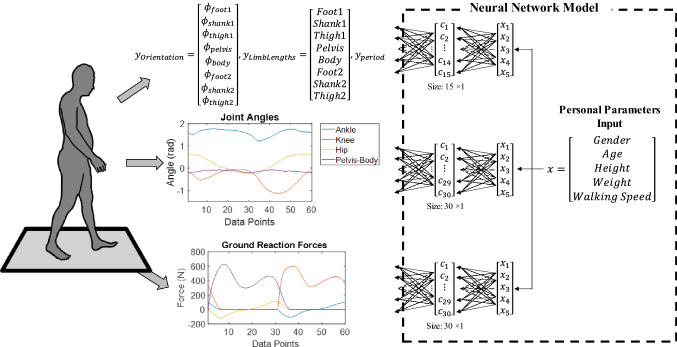
In this research, multilayer perceptron, a supervised neural network model, was used to capture nonlinear dynamics of personal parameters and gait behavior. An artificial neural networks-based gait characterization model was created to understand the effect of personal parameters (age, sex, height, weight, and walking speed) on walking behavior as well as to detect deviations from normal gait exhibited during a gait cycle as shown in Fig. 1. The input layer of the neural network model, , was the information about personal parameters. Output layers of the neural network model were gait parameters, for example orientation of body limbs during initial contact, lengths of each limb, joint angles, and GRFs.
Fig. 1.
Overview of the system. Motion capture experiments (schematic), outputs of the experiments, and corresponding neural network models
First, input vectors were created. There are five nodes in input layer for the information about sex, height, weight, age, and walking speed. Then, the vectors which describe limb lengths, body orientation of all limbs during the initial contact, and the period of the gait cycle have been created. Limb lengths and orientation vector contains eight nodes for each limb. The duration of the gait cycle, in other words period, has a single node. Separate neural network models were used for each output vector. When it comes to joint angles and GRFs, 6 different output vectors were created: joint angles of ankle, knee, hip, and pelvis-body joints, and GRFs in the horizontal and vertical axis. The dataset of each joint angle and GRFs in each direction were considered as the outputs of separate neural network models.
A total of 2250 gait cycles, 10 gait cycles for 225 subjects, were used. Output vectors were divided into train, test, and validation data with ratios of 60%, 20%, and 20%, respectively. Data were divided randomly into five groups and one of the groups was assigned as test data during fivefold cross-validation. The remaining 80% of them were distributed randomly into training and validation data. Train data was used to calculate gradient and update parameters. The early stopping technique was used to prevent overfitting. If the error in the validation data increases for a number of iterations, the training procedure stops. Performance function was determined as mean squared error (MSE) and calculated for train, test, and validation data. To measure the quality of learning, the coefficient of determination (R2) and MSE were checked for each model.
The number of nodes in the hidden layer was determined by using fivefold cross-validation. MSE, R2, and computational time for learning were obtained as given in Table 2. It was revealed that the increasing number of nodes in the hidden layer reduced MSE, and increased R and computational time. When the number of nodes in the hidden layer increases more, the gap between the MSE of the training group and the validation/test group increases. Therefore, further investigations related to the period, limb lengths, orientation, joint angles, and GRFs were carried out by considering a single hidden layer with 30 nodes not to increase computational cost more.
Table 2.
Mean values of MSE, R.2 and computational time for artificial neural network models with different configurations
| 5 nodes | 15 nodes | 30 nodes | |||
|---|---|---|---|---|---|
| Period | MSE | Train | 0.0015 | 0.0008 | 0.0004 |
| Valid | 0.0017 | 0.0011 | 0.0006 | ||
| Test | 0.0016 | 0.001 | 0.0006 | ||
| R2 | 0.7124 | 0.8253 | 0.9057 | ||
| Comp. Time (s) | 0.2263 | 0.3642 | 0.5568 | ||
| Limb Lengths | MSE | Train | 0.000142 | 0.000107 | 0.00007 |
| Valid | 0.000145 | 0.000116 | 0.000084 | ||
| Test | 0.000145 | 0.000116 | 0.000083 | ||
| R2 | 0.9923 | 0.994 | 0.9959 | ||
| Comp. Time (s) | 1.4087 | 2.9573 | 8.66 | ||
| Orientation | MSE | Train | 0.0048 | 0.0038 | 0.0027 |
| Valid | 0.0049 | 0.0041 | 0.0031 | ||
| Test | 0.0049 | 0.0041 | 0.0032 | ||
| R2 | 0.9877 | 0.9901 | 0.9927 | ||
| Comp. Time (s) | 0.9615 | 2.7845 | 11.1782 | ||
| Ankle Joint Angle | MSE | Train | 0.00257 | 0.00217 | 0.00168 |
| Valid | 0.00265 | 0.00239 | 0.00204 | ||
| Test | 0.00265 | 0.00237 | 0.002 | ||
| R2 | 0.8868 | 0.9019 | 0.9208 | ||
| Comp. Time (s) | 21 | 398 | 1425 | ||
| Knee Joint Angle | MSE | Train | 0.0042 | 0.00342 | 0.00252 |
| Valid | 0.00441 | 0.00378 | 0.00308 | ||
| Test | 0.00437 | 0.00378 | 0.00303 | ||
| R2 | 0.9632 | 0.9692 | 0.9764 | ||
| Comp. Time (s) | 31 | 262 | 1131 | ||
| Hip Joint Angle | MSE | Train | 0.00172 | 0.00137 | 0.00105 |
| Valid | 0.00186 | 0.00154 | 0.00128 | ||
| Test | 0.00179 | 0.00151 | 0.00126 | ||
| R2 | 0.9812 | 0.9847 | 0.9879 | ||
| Comp. Time (s) | 46 | 219 | 1034 | ||
| Pelvis-Body Joint Angle | MSE | Train | 0.00044 | 0.0004 | 0.00035 |
| Valid | 0.00044 | 0.00042 | 0.00038 | ||
| Test | 0.00045 | 0.00041 | 0.00039 | ||
| R2 | 0.7164 | 0.7397 | 0.7666 | ||
| Comp. Time (s) | 39 | 350 | 1510 | ||
| Vertical GRF | MSE | Train | 0.00355 | 0.00309 | 0.00257 |
| Valid | 0.00354 | 0.0032 | 0.00292 | ||
| Test | 0.00361 | 0.00332 | 0.00299 | ||
| R2 | 0.9832 | 0.985 | 0.9871 | ||
| Comp. Time (s) | 33 | 588 | 1555 | ||
| Horizontal GRF | MSE | Train | 0.00032 | 0.00029 | 0.00024 |
| Valid | 0.00034 | 0.00032 | 0.00028 | ||
| Test | 0.00033 | 0.00031 | 0.00027 | ||
| R2 | 0.9643 | 0.9669 | 0.972 | ||
| Comp. Time (s) | 27 | 209 | 1346 | ||
Results
Effects of the input vector on different outputs have been presented by using neural network models. First, separate neural network models between input and output vectors have been created to reveal how personal parameters affect gait parameters. Based on the models, output vectors have been generated using the same input vectors. The difference between experimental data and generated data shows how experimental data deviate from the predictions of the model.
Regression model of gait parameters
First, neural network models for the different gait parameters were created. 5-fold cross-validation was performed to determine the number of neurons in the hidden layer and it was determined to continue 30 neurons with a single hidden layer. The performance of the artificial neural network models was investigated by mean square error (MSE) and coefficient of determination R2.
The neural network model of the period has R2 of 0.9057 and MSE of 0.0006. It was expected to have high R2 and low MSE in limb lengths output due to the proportionality of the human body. As expected, R2 was more than 0.99 even with 5 nodes in a single hidden layer and increased till 30 nodes. MSE of the neural network model for ankle, knee and hip joint angles in test data was 0.002, 0.003, and 0.0012, respectively. R2 values of them were greater than 0.92. The neural network model of the pelvis-body joint had MSE of 0.00039 and R2 of 0.7666. It should be noted that MSE of pelvis-body joint angle was the lowest due to the low range of motion of the pelvis-body joint. R2 of ground reaction forces was more than 0.97.
In addition to R2 and MSE, the accuracies of the models in terms of physical units were obtained. For this purpose, the difference vectors were obtained by subtracting model prediction and experimental data. Mean values and standard deviations of the difference vectors for each gait parameter were given in Table 3.
Table 3.
Mean values and standard deviations of the difference vectors between model prediction and experiments
| Gait parameter | Mean value | Standard deviation |
|---|---|---|
| Period (s) | − 2.7 × 10⁻⁴ | 0.025 |
| Limb lengths (m) | 5 × 10⁻⁵ | 0.008 |
| Orientation (deg) | − 0.0171 | 3.09 |
| Ankle joint (deg) | 2 × 10⁻⁴ | 2.44 |
| Knee joint (deg) | − 3 × 10⁻⁴ | 3.06 |
| Hip joint (deg) | − 8 × 10⁻⁵ | 2.03 |
| Pelvis-body joint (deg) | − 3 × 10⁻⁷ | 1.12 |
| Vertical GRF (N/BW) | − 1 × 10⁻⁴ | 0.041 |
| Horizontal GRF (N/BW) | − 1 × 10⁻⁵ | 0.012 |
Effects of personal parameters on outputs
Period, orientation of limbs, length of limbs, joint angles, GRFs, etc. vary depending on subjects’ characteristics such as age, sex, average walking speed. To understand how each personal parameter affects output vectors, neural network models were simulated by changing only corresponding personal parameter and other personal parameters were kept same. It was revealed that period decreases with walking speed and other input parameters have a less significant effect on period. The orientations of the body limbs during initial contact were affected mostly by body height and walking speed.
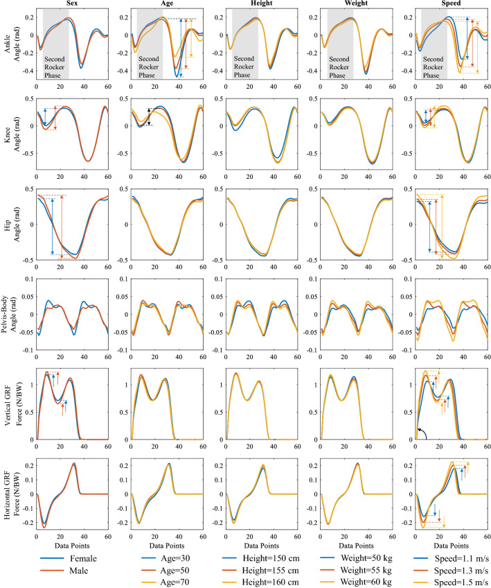
The effects of personal parameters on joint motion and GRFs were shown in Fig. 2. Joint angles were affected mostly by sex, age, and walking speed. It was estimated that female subjects have a slightly larger range of motion for the ankle joint, whereas male subjects have a larger range of motion for the hip joint. Male subjects have a larger knee flexion/extension during stance phase (between data points of 0–30) as shown in Fig. 2.
Fig. 2.
Effect of input parameters of sex, age, height, weight, and preferred walking speed on joint angles and ground reaction forces. The adaptations were marked by arrows
The effects of age on joint motion were evident especially in ankle and knee joints. Increasing age decreased the range of motion and affected the slope of joint motion during the second rocker phase (between data points of 5–30) in the ankle joint as shown in Fig. 2. It was also appeared that reduction in knee joint motion occurs during the stance phase (between data points of 0–30) when age increases according to Fig. 2.
Walking speed has the most prominent adaptations in joint angles. When walking speed increases, the range of motion of the ankle joint increases. Besides, the slope of the ankle joint changes during second rocker phase depending on walking speed. According to Fig. 2, the flexion and extension of the knee joint during the stance phase increase with walking speed. Figure 2 also shows that the range of motion in the hip joint also increases when walking speed increases. The hip joint moves faster during the stance phase when walking velocity increases. However, the slope of the curve during the swing phase does not change significantly.
When it comes to ground reaction forces, walking speed affects both vertical and horizontal GRFs, dramatically. When walking speed increases, the loading rate and amount of the first peak of vertical GRF increases. Similarly, the peak propulsive and braking GRF in the horizontal direction increases as shown in Fig. 2.
Level of deviations
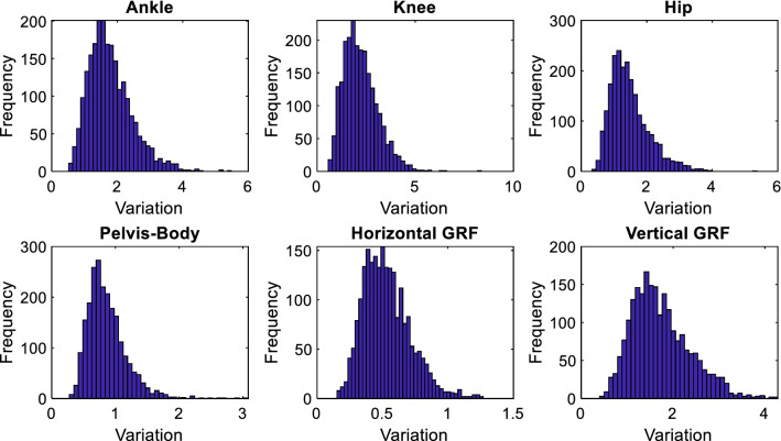
After modeling the tendencies of the gait parameters related to personal parameters, the differences between model predictions and experimental dataset were investigated for each output vector. Let and be experimental and neural network prediction of an output vector, such as knee joint angle with =60 data points. The deviation, , was defined as the summation of absolute values of the elements in the difference vector of each output as given in Eq. (1).
| 1 |
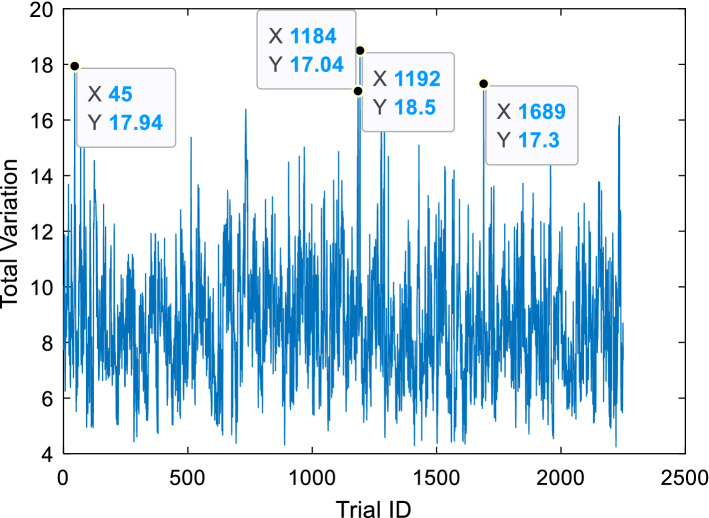
Thus, a scalar, , indicated how much difference occur between experiments and estimation of the artificial neural network model. The distribution of the deviations for each output was as given in Fig. 3. All of the distributions were right-skewed and there were few trials that contains an excessive amount of deviation. Then, total deviation was defined as the summation of the deviations in each output vector. A trial ID was assigned to each gait cycle. Trial ID’s and their total deviations were given in Fig. 4 and trials with maximum deviation were marked. Also, each component of the total deviation with trial ID was given in Table 4 for the trials with maximum deviations. Knee joint angle, hip joint angle, and vertical GRF contributed more than other temporal output vectors to total deviation for the trials with maximum deviations.
Fig. 3.
Distribution of the deviation in joint angles and GRF
Fig. 4.
Distribution of total deviation among trials. X and Y are trial ID and total deviation of the trial, respectively
Table 4.
Components of the total deviation in trials with maximum deviation
| Trial ID | Deviations | ||||||
|---|---|---|---|---|---|---|---|
| Ankle | Knee | Hip | Pelvis-body | GRF horizontal | GRF vertical | Total | |
| 1192 | 2.72 | 8.35 | 3.57 | 1.48 | 0.57 | 1.77 | 18.49 |
| 45 | 2.55 | 5.64 | 3.91 | 1.06 | 0.99 | 3.75 | 17.93 |
| 1689 | 3.28 | 6.42 | 2.67 | 0.77 | 0.96 | 3.17 | 17.3 |
| 1184 | 2.84 | 6.32 | 3.96 | 1.28 | 0.63 | 1.97 | 17.03 |
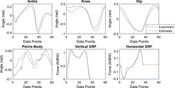
To illustrate what was performed in experiments and what was predicted by the artificial neural network model, joint angles, and GRFs of the trial with maximum deviation were given together in Fig. 5. The trial with maximum deviation, trial ID = 1192 (Female, Age 23 years old, Height 1.58 m, Weight 47 kg, and Speed 1.23 m/s), have large deviations in the joint angles and GRFs according to Table 4 and Fig. 5. It was predicted that the range of motion of the ankle joint to be lower. The difference in the knee joint motion during the stance phase is observed. Also, the loading rate of vertical GRF was predicted to be lower.
Fig. 5.
Experimental and neural network model generated data for joint angles and GRFs for the trial ID = 1192
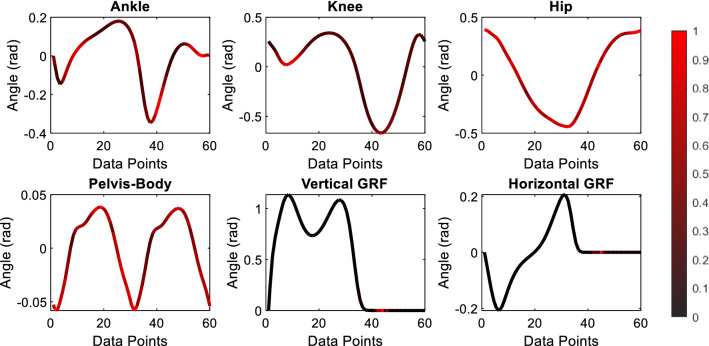
Another important topic is to understand where excessive differences intensify between model and experimental data. For this purpose, standard deviations of difference vectors were calculated at each data point. The interval of ± 3 standard deviations contain more than 99.5% of data by assuming normal distribution. If the difference was more than 3 standard deviations for a data point of an output vector, the data point was considered as outlier. The number of outliers for each data point was counted for all outputs. If data were distributed normally, it is expected to have no significant difference between data points. However, the existence of the considerable differences between model and experiments reveals where deviations occur commonly. Figure 6 shows where the differences between model and experiments were concentrated by using average joint angles and GRFs curves. A red to black gradient was used to express how frequent difference occurs more than three standard deviations. The number of outlier data was normalized for each output vector and the red color represents where the maximum difference occurs between predicted and experimental data.
Fig. 6.
The distribution of the high (more than 3 standard deviations) differences between model and experiments for joint angles and GRFs. Black to red gradient color shows the frequency of high difference
According to Fig. 6, the locations with red color contain more excessive differences than other locations. There are three regions where high differences occur mostly for ankle joints: second rocker phase, termination of the stance, and termination of the swing. In the second rocker phase, the foot is stationary on the ground and the thigh rotates around the ankle joint. The behavior of the ankle in the second rocker phase is useful to understand ankle joint characteristics. Termination of the swing is important to adjust foot orientation to touch the ground properly. The ratio of stance/swing time may cause excessive differences around termination of the stance for ankle joint, also GRFs. Knee joint data have one location with high deviation: weight acceptance phase. Knee joint motion during the weight acceptance phase is one of the indicators of several problems such as osteoarthritis, low back pain, etc. The range of motion for pelvis-body motion can be considered as another important parameter. Although the range of motion for the pelvis-body joint is important, it should be noted that the performance of the neural network was not so high. As a result, it can be said that neural network model predictions catch the behavior for joint angles and GRFs. Red areas are the phases where output vectors exhibit excessive differences.
Discussions
In this research, various gait parameters of the 225 subjects were obtained in 10 trials, which is equal to 2250 samples for each gait parameter in total. First, the effects of personal parameters on gait parameters were modeled by using artificial neural networks to identify normal walking that considers personal parameters. It can be said that all gait parameters except pelvis-body joint motion have good fitting performances with R2 more than 0.90.
The effects of personal parameters on joint angles and GRFs were modeled by using artificial neural networks. The artificial neural network model revealed the effects of personal parameters obtained in other studies on gait parameters collectively and individually. The neural network model predictions match with previous works [2, 5, 21]. The effects of walking speed on joint angles have similar behavior to previous research [21]. Similarly, the effects of age by using the neural network models have consistency with previous works on aging effect on the ankle and knee joint motion [2].
The artificial neural network models expressed the tendencies of the different gait parameters depending on the personal parameters. The neural network model of joint motion of pelvis-body joint has less accuracy in terms of the coefficient of determination, R2. The pelvis-body joint motion has less range of motion and is more sensitive to small errors compared to other joint motions. Also, small but sudden changes in spinal posture can cause a spiky joint angle curve that reduces the accuracy of the model. When the accuracy of models was considered in terms of physical units, standard deviation of the error in joint angles was around 3 degrees. The standard deviation of error was between 4 and 6 degrees in a similar previous study which uses multiple linear regression [20]. It can be said that the accuracy of the model is better than multiple linear regression model. Besides, the errors in the range of ± 5 degree were considered acceptable limits for clinical applications [22].
Another purpose of the study was to detect deviations from normal gait. The deviation, , was used for this purpose. According to Table 4 and Fig. 3, the deviation of knee joint angle of trial ID = 1192 is quite high in the population. The predicted motion and experimental data were given in Fig. 5. The deviation of knee joint angle is obvious, especially in loading phase of knee joint. In future research, a threshold level of deviation should be set to determine abnormality by including abnormal walking dataset.
The present study shows that artificial neural network models improve the accuracy of the normal gait prediction models. The effects of age, sex, weight, height, and walking speed on the human gait was obtained. Besides, the application of the neural network models on gait data can be further extended to understand adaptations such as slope walking, walking with additional mass, stair ascending/descending, and so on. Thus, predicted gait data can be used to design personalized walking assistive devices, orthoses, prosthetics, etc.
One of the drawbacks of the proposed method is the non-uniqueness of the outputs for a given personal parameter. It is expected to have variability in each gait parameter, therefore upper and lower bound should be determined in future studies to specify the range of normal gait.
Conclusion
The artificial neural network is a technique for classification, regression, and clustering problems. Recently, neural network applications of complex behavior of the human gait have gained attention. In this research, it is aimed to detect the variations of the subject’s gait behavior by considering personal parameters, such as age, sex, and walking speed. Neural network models were built to understand the relationship between personal parameters and gait parameters. The differences between neural network model estimations and experimental data were calculated. The effect of age, sex, height, weight, and walking speed on gait variables were discussed. The walking trails with excessive deviations were investigated deeply by considering the distribution of the deviations in each gait variable. It was revealed that a neural network-based motion characterization model can predict where excessive differences from normal gait occurred. Finally, the stages of walking where large deviations were intensified were shown.
Acknowledgements
We would like to thank Dr. Hiroaki Hobara for his comments and the contributions on discussions.
Author contributions
GC carried out the concept of the study, performed calculations and obtained results. SK and YK contributed to discussions of the method, model, and results. SS contributed to discussions. GC wrote the manuscript, SK, YK and SS read and reviewed the manuscript. All authors read and approved the final manuscript.
Funding
The authors declare that no funds, grants, or other support were received during the preparation of this manuscript.
Declarations
Competing interests
The authors declare that they have no competing interests.
Ethics approval
The study protocol of the publicly available AIST gait database was approved by the local ethical committee.
Informed consent
The written consent was obtained from all participants. (Source: https://unit.aist.go.jp/harc/ExPART/GDB2019.html).
Footnotes
Publisher's Note
Springer Nature remains neutral with regard to jurisdictional claims in published maps and institutional affiliations.
References
- 1.Danion F, Varraine E, Bonnard M, Pailhous J. Stride variability in human gait: The effect of stride frequency and stride length. Gait Posture. 2003 doi: 10.1016/S0966-6362(03)00030-4. [DOI] [PubMed] [Google Scholar]
- 2.Begg R, Sparrow W. Ageing effects on knee and ankle joint angles at key events and phases of the gait cycle. J Med Eng Technol. 2006 doi: 10.1080/03091900500445353. [DOI] [PubMed] [Google Scholar]
- 3.Judge JO, Ounpuu S, Davis RB., III Effects of age on the biomechanics and physiology of gait. Clin Geriatr Med. 1996 doi: 10.1016/S0749-0690(18)30194-0. [DOI] [PubMed] [Google Scholar]
- 4.Messier SP. Osteoarthritis of the knee and associated factors of age and obesity: effects on gait. Med Sci Sports Exerc. 1994;26(12):1446–1452. doi: 10.1249/00005768-199412000-00006. [DOI] [PubMed] [Google Scholar]
- 5.Røislien J, Skare Ø, Gustavsen M, Broch N, Rennie L, Opheim A. Simultaneous estimation of effects of gender, age and walking speed on kinematic gait data. Gait Posture. 2009 doi: 10.1016/j.gaitpost.2009.07.002. [DOI] [PubMed] [Google Scholar]
- 6.Kaufman KR, Hughes C, Morrey BF, Morrey M, An K. Gait characteristics of patients with knee osteoarthritis. J Biomech. 2001 doi: 10.1016/S0021-9290(01)00036-7. [DOI] [PubMed] [Google Scholar]
- 7.Filli L, Sutter T, Easthope CS, Killeen T, Meyer C, Reuter K, Lörincz L, Bolliger M, Weller M, Curt A, Straumann D, Linnebank M, Zörner B. Profiling walking dysfunction in multiple sclerosis: characterisation, classification and progression over time. Sci Rep. 2018 doi: 10.1038/s41598-018-22676-0. [DOI] [PMC free article] [PubMed] [Google Scholar]
- 8.Hausdorff JM. Gait dynamics in Parkinson's disease: common and distinct behavior among stride length, gait variability, and fractal-like scaling. Chaos. 2009;19(2):026113. doi: 10.1063/1.3147408. [DOI] [PMC free article] [PubMed] [Google Scholar]
- 9.Chu CR, Williams AA, Coyle CH, Bowers ME. Early diagnosis to enable early treatment of pre-osteoarthritis. Arthritis Res Ther. 2012;14(3):212. doi: 10.1186/ar3845. [DOI] [PMC free article] [PubMed] [Google Scholar]
- 10.Balasubramanian CK, Neptune RR, Kautz SA. Variability in spatiotemporal step characteristics and its relationship to walking performance post-stroke. Gait Posture. 2009;29(3):408–414. doi: 10.1016/j.gaitpost.2008.10.061. [DOI] [PMC free article] [PubMed] [Google Scholar]
- 11.Benedetti MG, Piperno R, Simoncini L, Bonato P, Tonini A, Giannini S. Gait abnormalities in minimally impaired multiple sclerosis patients. Mult Scler. 1999;5(5):363–368. doi: 10.1177/135245859900500510. [DOI] [PubMed] [Google Scholar]
- 12.Mills K, Hettinga BA, Pohl MB, Ferber R. Between-limb kinematic asymmetry during gait in unilateral and bilateral mild to moderate knee osteoarthritis. Arch Phys Med Rehabil. 2013;94(11):2241–2247. doi: 10.1016/j.apmr.2013.05.010. [DOI] [PubMed] [Google Scholar]
- 13.Craig JJ, Bruetsch AP, Lynch SG, Huisinga JM. The relationship between trunk and foot acceleration variability during walking shows minor changes in persons with multiple sclerosis. Clin Biomech. 2017;49:16–21. doi: 10.1016/j.clinbiomech.2017.07.011. [DOI] [PMC free article] [PubMed] [Google Scholar]
- 14.Zeni JA, Jr, Higginson JS. Dynamic knee joint stiffness in subjects with a progressive increase in severity of knee osteoarthritis. Clin Biomech. 2009;24(4):366–371. doi: 10.1016/j.clinbiomech.2009.01.005. [DOI] [PMC free article] [PubMed] [Google Scholar]
- 15.Hamill J, Moses M, Seay J. Lower extremity joint stiffness in runners with low back pain. Res Sports Med. 2009;17(4):260–273. doi: 10.1080/15438620903352057. [DOI] [PubMed] [Google Scholar]
- 16.Cimolin V, Galli M, Grugni G, Vismara L, Albertini G, Rigoldi C, Capodaglio P. Gait patterns in prader-willi and down syndrome patients. J Neuroeng Rehabil. 2010 doi: 10.1186/1743-0003-7-28. [DOI] [PMC free article] [PubMed] [Google Scholar]
- 17.Galli M, Rigoldi C, Brunner R, Virji-Babul N, Giorgio A. Joint stiffness and gait pattern evaluation in children with Down syndrome. Gait Posture. 2008;28(3):502–506. doi: 10.1016/j.gaitpost.2008.03.001. [DOI] [PubMed] [Google Scholar]
- 18.Wang TM, Huang HP, Li JD, Hong SW, Lo WC, Lu TW. Leg and joint stiffness in children with spastic diplegic cerebral palsy during level walking. PLoS ONE. 2015;10(12):e0143967. doi: 10.1371/journal.pone.0143967. [DOI] [PMC free article] [PubMed] [Google Scholar]
- 19.Kobayashi Y, Hida N, Nakajima K, Fujimoto M, Mochimaru M. AIST Gait Database 2019. 2019; https://unit.aist.go.jp/harc/ExPART/GDB2019.html
- 20.Moissenet F, Leboeuf F, Armand S. Lower limb sagittal gait kinematics can be predicted based on walking speed, gender, age and BMI. Sci Rep. 2019;9:9510. doi: 10.1038/s41598-019-45397-4. [DOI] [PMC free article] [PubMed] [Google Scholar]
- 21.Mentiplay BF, Banky M, Clark RA, Kahn MB, Williams G. Lower limb angular velocity during walking at various speeds. Gait Posture. 2018;65:190–196. doi: 10.1016/j.gaitpost.2018.06.162. [DOI] [PubMed] [Google Scholar]
- 22.McGinley JL, Baker R, Wolfe R, Morris ME. The reliability of three-dimensional kinematic gait measurements: A systematic review. Gait Posture. 2009;29:360–369. doi: 10.1016/j.gaitpost.2008.09.003. [DOI] [PubMed] [Google Scholar]


