Abstract
Karst is a common engineering environment in the process of tunnel construction, which poses a serious threat to the construction and operation, and the theory on calculating the settlement without the assumption of semi-infinite half-space is lack. Meanwhile, due to the limitation of test conditions or field measurement, the settlement of high-speed railway tunnel in Karst region is difficult to control and predict effectively. In this study, a novel intelligent displacement prediction model, following the machine learning (ML) incorporated with the finite difference method, is developed to evaluate the settlement of the tunnel floor. A back propagation neural network (BPNN) algorithm and a random forest (RF) algorithm are used herein, while the Bayesian regularization is applied to improve the BPNN and the Bayesian optimization is adopted for tuning the hyperparameters of RF. The newly proposed model is employed to predict the settlement of Changqingpo tunnel floor, located in the southeast of Yunnan Guizhou Plateau, China. Numerical simulations have been performed on the Changqingpo tunnel in terms of variety of karst size, and locations. Validations of the numerical simulations have been validated by the field data. A data set of 456 samples based on the numerical results is constructed to evaluate the accuracy of models’ predictions. The correlation coefficients of the optimum BPNN and BR model in testing set are 0.987 and 0.925, respectively, indicating that the proposed BPNN model has more great potential to predict the settlement of tunnels located in karst areas. The case study of Changqingpo tunnel in karst region has demonstrated capability of the intelligent displacement prediction model to well predict the settlement of tunnel floor in Karst region.
Subject terms: Civil engineering, Applied mathematics, Computational science
Introduction
Karst mainly refers to the dissolution of soluble rocks by water and various landscape phenomena on the underground and surface1. Karstification often leads to rock fracture, grooves, cavities, and surface depressions that are caused by the collapse at the top of the karst cavity, which will increase the difficulty and risk of tunneling2–7. China is a large karst country, with a karst area of 3.44 million km2, accounting for about one third of the land area8. The karst distribution area in Yunnan Province is 110,875 km2, accounting for 28.14% of the total area, mainly distributed in the Northwest and Northeast9–12. In recent year, China has constructed a number of high-speed railway tunnels, and some of these tunnels have encountered giant karst caves13–16. The giant karst caves have large volume, complex geology, and high engineering risk17–21. Thus, the research on karst is of great significance for the scientific construction and safe operation of the tunnel.
The scale, size and location of karst have different effects on the stability of karst tunnel12,22–24. Except these, the stability of surrounding rock around the tunnel when the karst tunnel is located at the side, bottom and front side of the tunnel have been systematically studied, and the results indicated that the most influential position appears in the karst cave at the bottom of the tunnel25,26. Many studies just made a qualitative analysis like the safety thickness between tunnel floor and karst27, the failure mode of tunnel with different sizes and positions of karst22–24, but the quantitative research of maximum settlement on tunnel floor is lacking.
Forecasting the settlement can be done through either physical or data-based models28,29. The karst position and scale are various, making it complex to build physical models that are sufficiently representative. These shortcomings have been addressed in recent years through advances in artificial intelligence, especially machine learning algorithms, that have greatly improved modelling and forecasting of settlement30–33.
Recently, Machine learning (ML) techniques have recently applied in geotechnical engineering and tunnel engineering applications34–36. And different ML techniques have been used to solve the problem like surrounding rock deformation37, rock slope stability analyses38, ground surface settlement39 and other engineering problems. Arsalan Mahmoodzadeh et al.40 have been developed hybrid algorithms to predict Mode-I rock fracture toughness and fivefold cross-validation was applied. Besides, researchers also proposed different approaches to forecast the construction time and costs of tunneling projects, such as statistical methods41–44, fault tree or event tree analysis, decision trees or risk matrixes45–47. Arsalan Mahmoodzadeh et al.48 using four machine learning methods including the linear regression (LR), Gaussian process regression (GPR), support vector regression (SVR), and decision tree (DT) with the grey wolf optimization (GWO) algorithm was used to fine-tune the models' hyper-parameters to predict geology, duration, and costs of tunnels construction.
Some new back-analysis techniques have been attempted for important geotechnical problems recently. Among them, the artificial neural network (ANN), genetic algorithm (GA) and simulated annealing algorithm (SAA) are becoming popular49,50. In particular, the ANN including BPNN owns stronger self-adaption, self-organization, self-study and nonlinear mapping ability, which can avoid the shortcomings of traditional feedback methods and is gaining increasing popularity in recent years. The BPNN model is based on a gradient search to determine its weights, leading a tendency to fall into local minima during the learning process and significantly influenced by the initialization of the weight51,52. Regularization method can control the size of the network weights to effectively limit the overfitting. However, Bayes is a predictor, all predictor models have the advantage of good generalization ability. Therefore, compared with other methods, such as L1/2 regularization53,54, Tikhonov regularization55, Dropout regularization56,57 the model after Bayesian regularization has better generalization ability58.
The Random Forest (RF) algorithm is a new machine learning technique proposed by Breiman in 200159. The RF model could effectively analyze the nonlinear, highly collinearity and mutual influence data, without assuming the mathematical form of the model in advance, which provides a new idea for predicting karst tunnel base settlement. This algorithm has been applied in biology60,61, soil science62,63, medicine64 et al., but the application in karst tunnel base settlement prediction is less. Machine learning algorithm with multiple hyperparameters should be optimized including RF model. At present, researchers commonly used optimization algorithm such as: genetic algorithm (GA), particle swarm optimization (PSO) algorithm and grid search (GS) algorithm. The amount of input data has a great influence on the optimization results of Genetic algorithm and swarm optimization algorithms, the grid search algorithm may not be effective65. Meanwhile, four kinds of common super-parameter optimization algorithm, PSO, GA, Differential evolution (DE), BO have been proposed in the process of model development for super parameter to adjust. The results show that the BO-RF model can in the shortest time and the highest accuracy forecast65. Therefore, the Bayesian algorithm has advantage to optimize the hyperparameters of RF that can greatly improve the efficiency of parameter regulation66.
According to the previous literature, a novel intelligent displacement prediction model, following the machine learning (ML) incorporated with the finite difference method, is developed to evaluate the settlement of the bottom of tunnel floor. A back propagation neural network (BPNN) algorithm and a random forest (RF) algorithm are used herein, while the Bayesian regularization is applied to improve the BPNN and the Bayesian optimization is adopted for tuning the hyperparameters of RF. The newly proposed model is employed to predict the settlement of Changqingpo tunnel floor, located in the southeast of Yunnan Guizhou Plateau, China. Numerical simulations have been performed on the Changqingpo tunnel in terms of variety of karst size, and locations. A data set based on the numerical results is constructed to evaluate the accuracy of models’ predictions. The correlation coefficients indicating that the proposed BPNN model has more great potential to predict the settlement of tunnels located in karst areas.
The intelligent prediction model for the maximum settlement of tunnel floor
Sources of intelligent prediction model
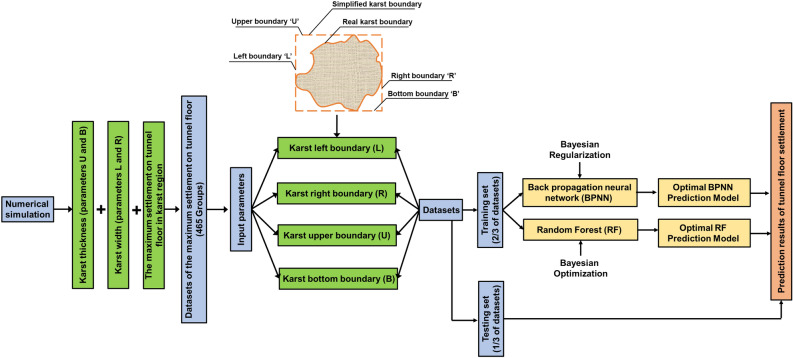
The dataset being interested in is the maximum tunnel floor settlement with various karst boundary. As shown in Fig. 1, karst boundary was simplified including upper, bottom, right and left boundary, they are represented by letters U, B, R and L. The karst could at the upper, bottom, right and left of tunnel, and for each of these positions the size of karst was also considered in this paper, which could be determined by these four kinds of karst boundary. Finite difference model could provide a tunnel floor settlement with various karst boundary dataset.
Figure 1.
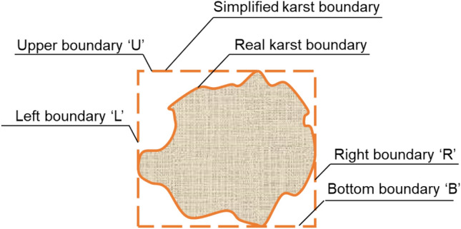
Simplified karst boundary.
The predicting process on tunnel floor settlement is as follows: the dataset could be collected from the numerical simulation that analysis the influences of karst size and position on the maximum tunnel floor and corresponding karst boundary parameters to form the dataset. The karst boundary parameters are selected as the variable matrix and the tunnel floor settlement as the response matrix. Two-third the size of dataset is selected at random as the training data and the rest as the testing set. Then, Bayesian regularization was used to enhance the generalization ability of BPNN and Bayesian optimization algorithm was applied to tune RF model’s hyperparameters. Through n-time model training, a BPNN and a RF regression model are obtained, which can be used to calculate the value of the new sample in testing set. The BPNN and RF modeling process is shown in Fig. 2. And the details on the process of the optimization are presented next.
Figure 2.
BPNN and BF model predicting process.
In regression analysis, mean square error (MSE), root mean squared error (RMSE), mean absolute error (MAE) and the correlation coefficient r, which are the most commonly used evaluation indicators. The r value is an indicator of the degree of correlation between variables. A positive r value means that the dependent variable increases with the independent variable, and the fitted straight line rises from left to right. The MAE is used to measure the average absolute error between the prediction value and the real value on the experimental data set, which cannot be used as loss functions in many cases. But MSE and RMSE could be used as a loss function, while RMSE is the square root of the MSE that has the same unit with output, which make it easy to analysis. Above all, the predictive performance of these two models could be evaluated using the root mean squared error RSME and the correlation coefficient r. And the RSME and r can be calculated by Eqs. (1) and (2):
| 1 |
| 2 |
where n is the number of samples, xi and yi are the experimental and predicted settlement values, respectively, and and represent the mean values of the experimental and predicted data, respectively.
BPNN with Bayesian regularization
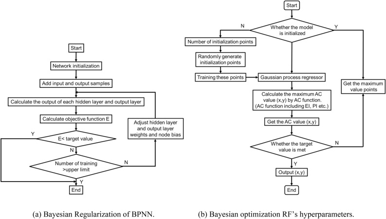
BPNN learning algorithm was used in this study to develop a mathematical equation relating the tunnel floor settlement to karst boundary. Input parameters are the karst boundary and output the value of corresponding settlement of tunnel floor. From a trial-and-error process, ten hidden neurons and the ‘sigmoid’ transfer function were found to be the optimal architecture. The implementation process of Bayesian regularization is shown in Fig. 3a. The calculation process of tunnel floor settlement ‘s’ using BPNN is elaborated in detail as Eqs. (3) to (6):
| 3 |
| 4 |
| 5 |
| 6 |
Figure 3.
Processes of optimization.
In which xi is the ith normalized input variable. bhk is the bias at neuron k (k = 1, 2, 3…14) of the hidden layer. whki is the weight connection between the neuron k of the hidden layer and the input variable xi (i = 1, 2, 3 …6). fsig is the sigmoid (tansig and purelin) transfer function. The ‘tansig’ was selected as the transfer function for the hidden layer to the output layer. The ‘purelin’ was selected as the transfer function for output layer to target. wok is the weight connection between the neuron k and the single output neuron. b0 is the bias of the output layer. s is the predictive result of tunnel floor settlement.
RF with Bayesian optimization of hyperparameters
Parameter adjustment is a tedious and essential step in machine learning. Since there are many hyperparameters in every model, which together affect the accuracy of these models. Thus, manually parameter adjustment could not make the algorithm achieve the best. However, The Bayesian optimization, a mathematical method, was introduced to automatically adjust parameters in this study. The Bayesian optimization algorithm is an approximation idea that the minimum value of the objective function is found by establishing substitution function (probability model), which based on the pervious evaluation results of the objective function67,68. Therefore, it can be used effectively when the calculation is very complex and the number of iterations is large69. Compared with Grid Search70 and Random Search71, Bayesian theorem is adopted in Bayesian optimization algorithm to estimate the posterior distribution of the objective function, and then, according to the distribution, the hyperparameter combination of the next sampling was selected. The optimization is a work to find the parameters, which maximize the global result by learning the shape of the objective function. The implementation process of Bayesian optimization is shown in Fig. 3b.
As all Bayesian methodologies, it is assumed Eq. (7):
| 7 |
where f (x) is a Gaussian process model that can evaluate yi according to each point xi, which was taken at random within the variable bounds. Then repeating updating the Gaussian process model of f (x) to obtain a posterior distribution over functions Q (f |xi, yi) until finding the point x that maximizes the acquisition (AC) function a(x).
In terms of RF model hyperparameters, due to the algorithm generally contains one or more important hyperparameters, Bayesian optimization algorithm is adopted to automatically search the optimal solution through learning the data samples, so as to optimize the prediction effect of the model. In the RF model, the hyperparameter including: the number of decision trees (n_estimators), The minimum number of samples required to split internal nodes (min_samples_split), the number of features to consider when looking for the optimal split point (max_features)72.
Ideally, if the sufficient data was obtained, the best practice is to randomly divide the dataset into three parts: a training set, a validation set, and a testing set. The training set is used to fit the models; the validation set is adopted to estimate prediction error for model selection; while the testing set is utilized for assessment of the generalization error of the finalized model73. Since data are generally scarce, the inability to truly reflect the generalization performance of the model is common. To avoid bias in data selection, one of the most popular validation methods, such as k-fold CV74–78. Because k-fold cross validation can be used to evaluate the prediction performance of the model, especially the performance of the trained model on new datasets, and the over-fitting can be reduced in some degree79. Thus, the results of each part of the samples can be output by the K-fold cross-validation method to solve the over-fitting problem. fivefold was adopted herein (see Fig. 4).
Figure 4.
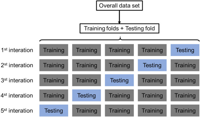
5-Fold cross-validation process.
Changpingpo tunnel: a case study
Engineering background
Changqingpo tunnel is in an edge slope area in the southeast of Yunnan Guizhou Plateau, connecting Puzhehei and Zhulin. The total length of the tunnel is 12.675 km. It is a double track high-speed railway tunnel. The designed clear height of the tunnel is 11.6 m and the width is 14.2 m. According to the operating speed requirements of high-speed railway trains, and the designed train operation speed is 200 km/h, and the reserved train operation speed is 250 km/h.
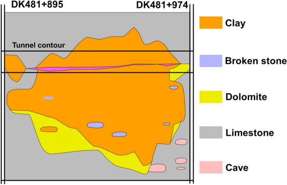
There are karst fillings in the range of the lowest karst which is 43 m above the tunnel floor according to the results of drilling and exploration. According to the engineering geological exploration report of Changqingpo tunnel, the main karst development of tunnel passing though was presented in Fig. 5, blow the tunnel floor, the karst cave is filled with clay, and from the experimental and standard data, the main composition of karst fillings is clay in the consistence plastic state, which contains a small amount of breccia unevenly (about 12%) and a very small amount of gravel.
Figure 5.
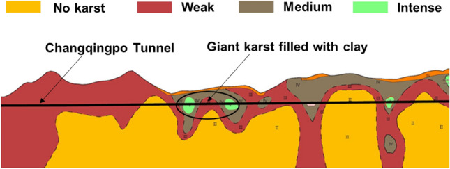
The main karst development of tunnel passing though.
The formation of Changqingpo Tunnel from DK483 + 978 to DK483 + 907 is mainly characterized that broken stone and clay are filled in the karst and dolomite and limestone of Upper Maping Formation (C3m) in Carboniferous is below the karst, and Table 1 describes the strata information. Figure 6 shows the schematic diagram of Changqingpo Tunnel of Yun-Gui Railway.
Table 1.
The strata information of Changqingpo Tunnel from DK483 + 978 to DK483 + 907.
| Strata sequence | Type | Condition | Thickness/m | Description |
|---|---|---|---|---|
| < 1–6 > | Filling (Q4ml) | Filling soil | 0 ~ 1 | Filling soil, mainly with concrete |
| < 2–11 > | Clay (Q4ca) | The distribution of soft and hard soil is irregular, mainly in hard plastic state, and partially in soft plastic state | 0 ~ 43 | The filling material of karst cave is mainly clay soil, which is gray black, yellow relatively uniform soil, and a small amount of local embedded gravel breccia |
| < 2–11–1 > | Broken stone | It is mainly filled with block stones | 0 ~ 3 | Karst cave filling material is mainly lump stone, which is gray white, and lump stone is locally distributed in clay of < 2–11 > |
| < 16–1 > | Limestone (C3m) | The joints are well developed, the dissolution erosion is serious, and the local erosion is very serious | 0 ~ 16 | The color of limestone is ashy, gray, which has thick layer massive structure and cryptocrystalline structure. It is the integrated contact with Weining Group below |
Figure 6.
The schematic diagram of Changqingpo Tunnel.
Model simulations
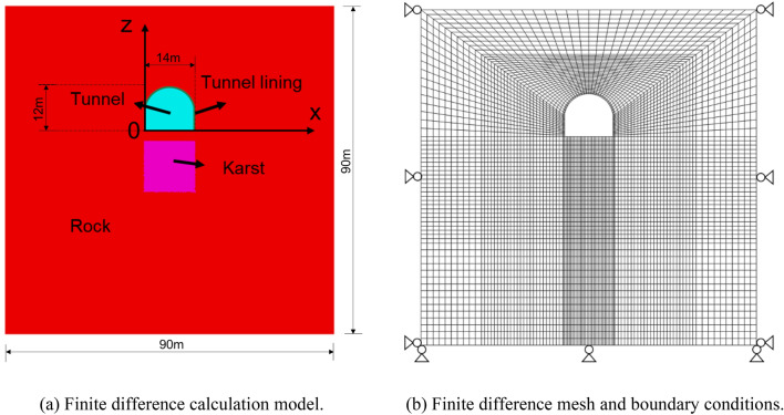
In order to eliminate the influence of boundary effect25, the model size is 6 times the tunnel diameter, the model dimension is 90 m × 90 m × 1 m. The tunnel adopts straight walls to connect the semicircular arch, which height is 12 m and width is 14 m, the thickness of tunneling lining is 0.5 m. Figure 7a shows the model diagram. Figure 7b illustrates the finite difference mesh for the numerical analysis, in which there are 6380 grids composed of 13,094 grid points. In the calculation model, lateral displacement boundaries were set in the X and Y direction. At the bottom of the model, the displacements in the X, Y and Z directions were restricted. The other surfaces were free.
Figure 7.
Finite difference model and mesh.
The Mohr Coulomb constitutive model is adopted for the filling soil and rock, the tunnel lining is linear elastic constitutive model. A uniform load of 200 kN/m is applied on the tunnel floor to simulate the railway load to analyze the final settlement of the tunnel floor.
According to the report of engineering geological exploration, the karst is filling with clay, the weight, cohesion, internal friction angle, young modulus and Poisson’s ratio of the cave filling are 12.5 kN/m3, 23 kPa, 20°, 22.7 MPa and 0.35, respectively. The rock around the tunnel occurred mainly in dolomite and limestone deposit of Mapping Group Upper Carboniferous system, the weight, cohesion, internal friction angle, young modulus and Poisson’s ratio of the rock are 27 kN/m3, 1500 kPa, 45°, 7.5 GPa and 0.28, respectively. Table 2 lists the actual rock and soil mechanics parameters were selected from a field survey report.
Table 2.
Parameter values adopted in this study.
| Type | ρ (g/cm3) | φ (°) | c (kPa) | μ | E (MPa) | Es (MPa) | K (MPa) | G (MPa) |
|---|---|---|---|---|---|---|---|---|
| Clay | 1.35 | 20 | 23 | 0.35 | 22.7 | 4.54 | 8. 4 | 25.22 |
| Rock | 2.7 | 45 | 1.5 × 10³ | 0.28 | 7.50 × 10³ | – | 2.93 × 10³ | 5.68 × 10³ |
| Tunnel lining | 2.8 | – | – | – | – | – | 1.12 × 10³ | 3.73 × 10³ |
The variables in this numerical study can be classified into five groups by (1) effects of karst on different positions of tunnel floor; (2) location of karst; (3) karst thickness; (4) karst width; (5) quality of rock mass around the tunnel and karst.
To study the influences of karst on different positions of tunnel floor and to compare the settlement of tunnel floor with different positions, varying sites were monitoring. Altogether, 27 monitoring sites were carried out of each value of U, the details of which are given in Table 3. According to the results of effects of karst on different positions of tunnel floor, the position with the maximum settlement on tunnel floor was regarded as the monitoring site in the study of the influences of karst locations, thickness, and width. Altogether, 37 cases were carried out, the details of which are given in Tables 4, 5, and 6, respectively.
Table 3.
Details of the effects of karst on different positions of tunnel floor.
| Case | L | R | U | B | Monitoring site (x-coordinate) |
|---|---|---|---|---|---|
| 1 | − 38 | 52 | 2 | 22 | 0.5, 1, 1.5, 2, …, 13.5 |
| 2 | 3 | 23 | 0.5, 1, 1.5, 2, …, 13.5 | ||
| 3 | 4 | 24 | 0.5, 1, 1.5, 2, …, 13.5 | ||
| 4 | 5 | 25 | 0.5, 1, 1.5, 2, …, 13.5 |
Table 4.
Details of the effects of karst locations on tunnel floor.
| Case | Location | Distance with the tunnel/m | Thickness of karst/m | Width of karst/m |
|---|---|---|---|---|
| 1 | Up | 1 | 14 | 14 |
| 2 | 2 | |||
| 3 | 3 | |||
| 4 | Down | 1 | 14 | 14 |
| 5 | 2 | |||
| 6 | 3 | |||
| 7 | Right | 1 | 14 | 14 |
| 8 | 2 | |||
| 9 | 3 |
Table 5.
Details of the effects of karst thickness.
| Case | L | R | U | B | Thickness of karst (B–U)/m | Width of karst (R–L)/m |
|---|---|---|---|---|---|---|
| 1 | − 38 | 52 | 0 | 0 | 0 | 0 |
| 2 | 1 | 2, 3, 4…21 | 1 ~ 20 | 90 | ||
| 3 | 2 | 3, 4, 5…22 | 1 ~ 20 | 90 | ||
| 4 | 3 | 4, 5, 6…23 | 1 ~ 20 | 90 | ||
| 5 | 5 | 6, 7, 8…25 | 1 ~ 20 | 90 | ||
| 6 | 10 | 11, 12…30 | 1 ~ 20 | 90 | ||
| 7 | 15 | 16, 17…35 | 1 ~ 20 | 90 | ||
| 8 | 20 | 21, 22…40 | 1 ~ 20 | 90 | ||
| 9 | 0 | 14 | 3 | 4, 5…43 | 1 ~ 40 | 14 |
| 10 | 5 | 6, 7…45 | 1 ~ 40 | 14 | ||
| 11 | 10 | 11, 12…50 | 1 ~ 40 | 14 | ||
| 12 | 15 | 16, 17…55 | 1 ~ 40 | 14 |
Table 6.
Details of the effects of karst width.
| Case | L | R | U | B | Thickness of karst (B–U)/m | Width of karst (R–L)/m |
|---|---|---|---|---|---|---|
| 1 | − 5 | − 4, − 3…52 | 1 | 5 | 4 | 1 ~ 57 |
| 2 | − 2 | − 1, 0, 1…52 | ||||
| 3 | 0 | 1, 2, 3…52 | ||||
| 4 | 2 | 3, 4, 5…52 | ||||
| 5 | 3 | 4, 5, 6…52 | ||||
| 6 | 5 | 6, 7, 8…52 | ||||
| 7 | 6 | 7, 8, 9…52 | ||||
| 8 | 7 | 8, 9…52 | ||||
| 9 | 8 | 9, 10…52 | ||||
| 10 | 9 | 10, 11…52 | ||||
| 11 | 10 | 11, 12…52 | ||||
| 12 | 12 | 13, 14…52 |
Besides these, the Rock mass quality Q of karst region was also considered. Additionally, it should be noted that the Q value cannot be directly used in the numerical calculation. The rock mass mechanical parameters are determined from the Q value by mean of the empirical relationship listed in Table 7. The values of Q were selected and its corresponding mechanical parameters to be used in the numerical analysis. Altogether, 10 cases were carried out, the details of which are given in Table 8.
Table 7.
Empirical equations relating Q with rock mass properties.
| Parameters | Relationship | References |
|---|---|---|
| Q | Q | |
| RMR | RMR = 7lnQ + 36 | Tugrul (1998)80 |
| Cohesion (kPa) | c = 5 × (RMR − 1) | Bieniawski (1989)59,81 |
| Internal friction angle φ (°) | φ = 0.5RMR + 4.5 | Bieniawski (1989)59,81 |
| Young’s modulus E (GPa) | E = 2 × RMR − 100 (RMR > 50) | Bieniawski (1978)82, Serafim and Pereira (1983)83 |
| E = 10(RMR − 10)/40 (RMR ≤ 50) | Bieniawski (1978)82, Serafim and Pereira (1983)83 |
Table 8.
Mechanical parameters of rock mass with different Q values.
| Case | Q value | Young’s modulus E (GPa) | Cohesion (kPa) | Internal friction angle φ (°) | Poisson ratio μ |
|---|---|---|---|---|---|
| 1 | 0.1 | 1.77 | 94.41 | 14.44 | 0.40 |
| 2 | 0.5 | 3.38 | 150.74 | 20.07 | 0.38 |
| 3 | 1 | 4.47 | 175.00 | 22.50 | 0.37 |
| 4 | 2 | 5.91 | 199.26 | 24.93 | 0.36 |
| 5 | 5 | 8.54 | 231.33 | 28.13 | 0.35 |
| 6 | 10 | 11.30 | 255.59 | 30.56 | 0.33 |
| 7 | 20 | 14.94 | 279.85 | 32.99 | 0.25 |
| 8 | 40 | 19.75 | 304.11 | 35.41 | 0.24 |
| 9 | 60 | 29.32 | 318.30 | 36.83 | 0.22 |
| 10 | 80 | 33.35 | 328.37 | 37.84 | 0.20 |
Parameter analysis
Validation of finite difference method
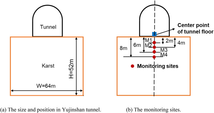
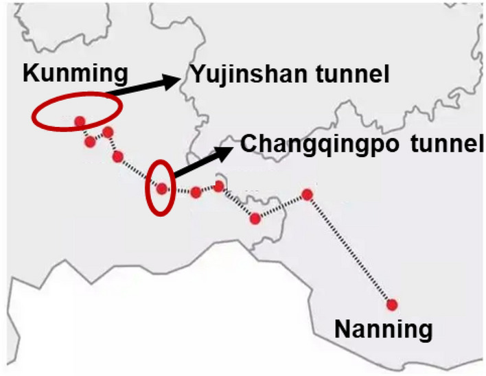
The validation of finite difference method was demonstrated through modeling the near engineering of Yujinshan tunnel84, which is in the northeast of Yunnan Province and has the same size of tunnel. The relative location of Changqingpo tunnel and Yujinshan tunnel is shown in Fig. 8. The material models and size of tunnel are presented is same as that given in Table 2. To achieve a calculate of tunnel floor settlement, a load due to machine drilling is 200 kPa was applied to the tunnel floor and the value of karst upper boundary is zero, also the thickness and the width of karst is 52 m and 64 m respectively as presented in Fig. 9a. The monitoring sites are shown in Fig. 9b.
Figure 8.
The relative location of Changqingpo tunnel and Yujinshan tunnel.
Figure 9.
The numerical model and monitoring sites.
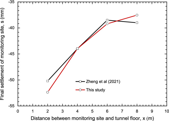
The result was compared with the monitoring data as shown in Fig. 10. Good agreement was obtained as presented in Fig. 10. Note that due to the influence of the grouting hole at the bottom of the tunnel and the rolling back and forth of construction vehicles, the final settlement decreased with the increase of depth in both two curves, and the maximum settlement of these two curves was 50.2 mm and 52.36 mm respectively on the M1, while the minimum settlement of these two curves was 39 mm and 37.54 mm respectively on the M4. Beside these, the value of settlement in Zheng et al. is smaller than that in finite difference method, and on the contrary, the settlement in Zheng et al. is larger. Note that the relative error is in a range of 0.045–4.3%, so the resulting value of settlement produced by the finite difference method were acceptable.
Figure 10.
The numerical model and monitoring results.
Effects of karst on different positions of tunnel floor
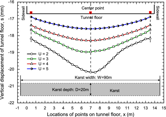
The karst located on the bottom of tunnel was firstly considered. For the giant karst cave, in order to study the effect of karst depth, the karst width was 90 m, which made left and right boundaries of karst coincided with model boundaries, considering the difference of karst thickness and upper boundary of karst, analyzing the influence of karst and the distance between tunnel floor and karst cave on the settlement of tunnel floor. The calculation results are shown in Fig. 11.
Figure 11.
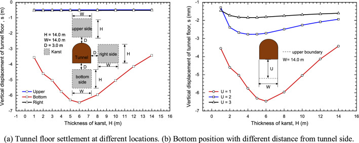
Tunnel floor settlement at different locations.
The settlement with different locations on tunnel floor was studied with varieties values of U. Considering that the karst thickness remains unchanged at 20 m and value of U is in the range of [2, 5], the settlement at different positions of tunnel floor was calculated. As shown in Fig. 11, the curve is in "V" shape, and the settlement increases from the corner of the tunnel to the middle. The settlement at the center is the largest, while at the corners are smaller than their neighbors. With the increasing of U, all curves tend to be gentle, and the settlement at the center of tunnel floor decreases gradually, which means the effect of karst gradually weakens.
Effects of karst position
In order to study influences of karst’s positions, three locations including upper, bottom and right of the tunnel were calculated respectively. The karst size remains 14 m × 14 m, and the karst center coincides with the tunnel centerline. Meanwhile, the influence of settlement at tunnel floor center with varieties distance between the karst boundary and the tunnel was researched, including U = 1, 2 and 3 respectively. As shown in Fig. 12.
Figure 12.
The influences of karst positions.
From the Fig. 12a, When the karst is located at the bottom of tunnel floor, the influence on the settlement is obvious, while the karst is located on right and top of the tunnel, the effect is weak25,26. At the same time, when the karst thickness remains unchanged, the settlement decreases gradually with the distance of karst and tunnel. If the karst is located below the tunnel floor, the curve presents a "V" shape as shown in Fig. 12b. With the increase of the karst thickness, the settlement first increases until thickness is 6 m and then decreases. With the growing of U, the settlement decreases gradually, and the curve tends to be flat.
Effects of karst thickness
The settlement of the center of tunnel floor was calculated including U = 2, 3, 5, 10, 15 and 20 while the karst thickness is a value in the range of (0, 20] and the width of karst is 90 m. It can be seen from Fig. 13 that when the width of karst is huge, the settlement of tunnel floor increasing with the growing of karst thickness. Considering the influence of U is in the range of [− 5, − 1], the curve presents a concave shape. With the increase of U, the curve tends to be a straight line. When U = 15 and U = 20, curves are basically coinciding, and the influence of U on the tunnel floor settlement could be ignored. In other words, if the karst thickness is unchanged, the effect of U on the tunnel floor settlement cannot be considered while U ≥ 15, which U is two times larger than excavating radius85.
Figure 13.
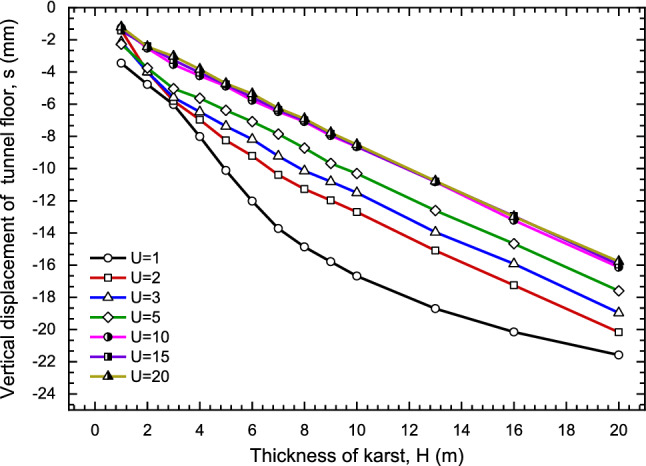
The effect of giant karst depth on tunnel floor settlement.
Then, for the usual size of karst (karst width is 14 m) as shown in Fig. 14, the influence of karst thickness become slight if karst thickness is larger 5 m. The impacts of U and B on the settlement were also analyzed. Under this condition, left boundary (L = 0) and right boundary (R = 13) are fixed, the relationship between karst thickness and settlement with different U is described in Fig. 15. With the decreasing of U, the settlement decreases gradually, and the settlement increases first and then decreases with the growth of thickness. Especially U = 10 and 15, curves tend to horizontal.
Figure 14.
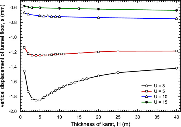
The effect of karst thickness and upper boundary.
Figure 15.
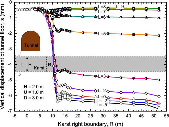
The effect of karst width (L and R) on tunnel floor settlement.
Effects of karst width
The effect of karst width could be considered as effects of L and R, as shown in Fig. 15, the x-coordinate of the tunnel center point is 7, and the upper boundary (U = 1) and bottom boundary (B = 3) are fixed for karst with usual size, the impacts of the left and right boundaries on the central settlement of tunnel floor were studied. From Fig. 15, the shape of the curve is similar to the word ‘Z’. When R < 7, karst has little impact on tunnel floor settlement. With the increasing of R, the settlement gradually increases and finally tends to be stable.
When L ≥ 7 or L < R < 7, these curves are essentially coincident and the values of settlement are all smaller than 1 mm so that the influence of karst on settlement cannot be considered. On the contrary, if L < 7 and R ≥ 7, the impact of karst on settlement is obvious. With the decrease of L, the maximum settlement growing and with the increase of R, settlement tends to stable after increase to the maximum. Finally, in the process of L and R change, when the tunnel floor center is located on the middle of L and R, the settlement at this position is the largest.
Effects of rock mass quality
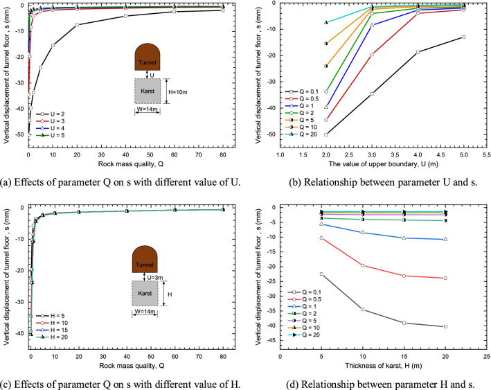
Figure 16a,b shows the variation curve of the rock mass quality with the maximum settlement of tunnel floor when U is 2, 3, 4 and 5, respectively. Also, there is the relationship between the rock mass quality Q and the maximum settlement of tunnel floor when the value of karst thickness is 5 m, 10 m, 15 m and 20 m respectively as presented in Fig. 16c,d.
Figure 16.
The Effects of rock mass quality Q on the maximum settlement of tunnel floor.
According to Fig. 16a, the maximum settlement s of tunnel floor quickly decreases with the increase of rock mass quality Q. Also, with the increase of U, the effects of the rock mass quality Q on the s gradually decreases, as described in Fig. 17b. In addition, it can be found the maximum settlement s of tunnel floor decreases rapidly with the increase of the rock mass quality Q. This shows that under the same conditions of karst boundary, the maximum settlement s of tunnel floor has little affected by the rock mass quality Q in the tunnel site when Q ≥ 5.
Figure 17.
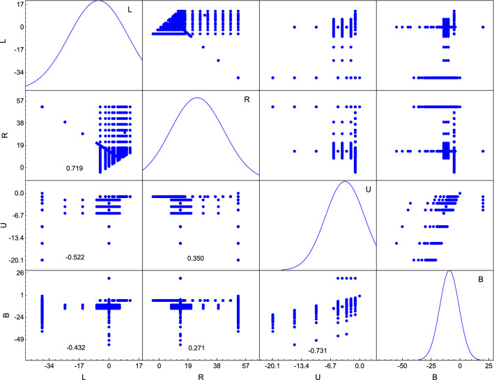
Distributions and correlation coefficients of model input variables in the data set.
Figure 16c,d shows the relationship between the maximum settlement s of tunnel floor and the rock mass quality Q under different H values. It is observed that the maximum settlement s of tunnel floor rapidly decreases with the increase of rock mass quality Q when 0 < Q < 5. On the contrary, when the rock mass quality Q ≥ 5 in the tunnel site, the maximum settlement s of tunnel floor is basically unchanged. In addition, there is little effect on the maximum settlement s of tunnel floor when the thickness of karst H is above 15 m, which is correspond to the results of Fig. 14.
Predicting results
Original input variables analysis and prediction models’ parameters
According to the results of influences of Q on s, in the region with Q ≥ 5, the maximum settlement of tunnel floor has been little affect by Q, and the mainly parameters are the karst boundaries including L, R, U and B.
The distributions of four boundaries of karst that were used in the prediction of tunnel floor maximum settlement are illustrated in the diagonal line of Fig. 17. The vertical axis of the diagonal histogram represents the frequency. The upper triangle reveals the pairwise correlation of the model input variables. The correlation coefficients are reported in the lower triangle. Most of the parameters are distributed in a concentrated manner. According to Koo and Li86, the r values less than 0.5, between 0.5 and 0.75, between 0.75 and 0.9, and greater than 0.90 are indicative of poor, moderate, good, and excellent reliability, respectively. There was moderate correlation between L and R, U and B, which was due to R is greater than L, and similarly, U is greater than B. There were relatively poor correlations between most input parameters (r < 0.5).
Optimization of intelligent prediction models
In prediction model, input parameters are the karst boundary of L, R, U and B and output value is the corresponding settlement of tunnel floor from FLAC3D. Of the 456 data sets, 340 patterns were randomly selected as the training data and the remaining 116 data were used for testing. According to the Eqs. (3) to (6), the BPNN model with Bayesian Regularization could be established, and Table 9 presents the connection weights and bias of the optimal network. As for RF model, the hyperparameters and its default value are listed in Table 10.
Table 9.
Connection weights and bias.
| ki | whki | wok | bhk | b0 | |||
|---|---|---|---|---|---|---|---|
| 1 | 2 | 3 | 4 | ||||
| 1 | 4.2605 | 3.4554 | 3.7972 | − 8.1639 | 2.7255 | 1.7510 | 1.9017 |
| 2 | 20.9391 | − 0.2385 | 1.7936 | − 6.0430 | 0.5745 | 14.2413 | |
| 3 | 3.5439 | − 8.9283 | − 6.6688 | − 0.1692 | 67.0555 | 3.5777 | |
| 4 | 3.3531 | − 8.8539 | − 6.6780 | − 0.1178 | 67.1183 | 3.4105 | |
| 5 | 0.2498 | 20.6089 | 4.6577 | 17.0069 | 0.8506 | 10.7792 | |
| 6 | 6.7630 | 24.7395 | 13.5221 | 1.1696 | 0.3237 | 4.5857 | |
| 7 | 7.1056 | 23.4865 | 25.4642 | 4.9186 | 0.3883 | 32.4610 | |
| 8 | 9.9134 | 9.5168 | 14.3857 | 2.8671 | 4.9222 | 0.2841 | |
| 9 | 11.4950 | 11.6263 | 33.6791 | 11.1526 | 0.3830 | 31.0921 | |
| 10 | 4.3978 | 3.8841 | 2.0611 | 5.1418 | 6.5138 | 7.5623 | |
Table 10.
Hyperparameter optimization.
| Condition | n_estimators | min_samples_split | max_features |
|---|---|---|---|
| Default | 100 | 2 | Auto |
| Optimal | 70 | 13.0865 | 2 |
Predicting results
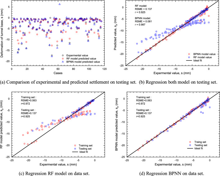
RMSE and r were selected as evaluation indexes. The evaluation of the BPNN and RF models were performed on both training set and testing set as shown in Table 11. The general predictive performance of the BPNN and RF models with optimum hyperparameters on training set was quite acceptable (Fig. 18). Figure 18a provides a visual comparison of predicted and experimental settlement values in testing set, indicating that predicted values are both relatively consistent with experimental values in BPNN and RF. The results of regression analysis of predicted and experimental settlement values in testing set are shown in Fig. 18b. Most points fell around the ideal fitting line, and values of r between the experimental and predicted settlement values of BPNN and RF model were 0.987 and 0.925, respectively. As suggested in previous studies, a model with r values larger than 0.8 can be regarded as acceptable87,88. In testing set, although r value of BPNN is 0.987, which is smaller than that of RF model and has great potential for making more reliable predictions. The RMSE of the BPNN and RF model with optimal hyperparameters was 0.081 and 0.137, also indicating that relatively good models had been achieved on the testing set.
Table 11.
Error comparison between BPNN and RF model.
| Predictive model | Correlation coefficient ‘r’ | RMSE | |
|---|---|---|---|
| BPNN | Training set | 0.972 | 0.016 |
| Testing set | 0.925 | 0.081 | |
| RF | Training set | 1.000 | 0.063 |
| Testing set | 0.987 | 0.137 | |
Figure 18.
Experimental versus predicted tunnel floor settlement for the BPNN and RF model on data set.
The results of regression analysis of predicted and experimental settlement values in both training and testing set are shown in Fig. 18c,d. Most points fall around the ideal fit line, and r values of BPNN and RF model are both larger than 0.9 in training set, which are 0.972 and 1.0 respectively. The RMSE of the BPNN and RF model in training set were 0.016 and 0.063.
Relative importance of karst boundaries
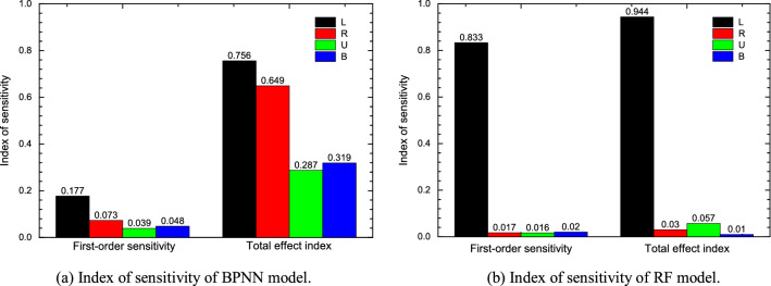
The tunnel floor settlement under load with different karst spatial distribution was studied by established BPNN and RF models to predict the settlement. The variation interval of each parameter is set to fluctuate up and down within the size range of the numerical model, and the probability distribution of each parameter is assumed to be uniform distribution. The optimal Latin hypercube design is used to sample each parameter, and the sampling results are applied to the prediction model. According to the sensitivity index calculation method based on Sobol method provided by Saltelli89, the first-order sensitivity index and total effect index of each parameter of the three prediction models are calculated respectively. The calculation results are shown in Table 12.
Table 12.
Results of relative importance analysis.
| Method | Parameter | First-order sensitivity S | Total effect index ST |
|---|---|---|---|
| BPNN | L | 0.177 | 0.756 |
| R | 0.073 | 0.649 | |
| U | 0.039 | 0.287 | |
| B | 0.048 | 0.319 | |
| RF model | L | 0.833 | 0.944 |
| R | 0.017 | 0.030 | |
| U | 0.016 | 0.057 | |
| B | 0.020 | 0.100 |
The ability to investigate the relative importance of the influencing variables is another crucial reason why the model is widely used in prediction problems. It can be used to rank the influencing variables according to their contribution to the performance of the prediction model. To reveal the effect of influencing variables on the predicted settlement values of tunnel floor, a sensitivity analysis was conducted for these influencing variables.
Comparing the first-order sensitivity index and total effect index of each parameter in two models as shown Table 12, the first-order sensitivity index and total effect index of L is the largest in the corresponding sensitivity index. In the RF model, the first-order sensitivity index and total effect index of L are significantly greater than the corresponding sensitivity indexes of the other three parameters that means both the influence of a single parameter on the output variance of the model or the total influence of a parameter on the output variance, the change of L has the greatest influence on the settlement of the tunnel floor. Therefore, the small variation range of L is the reason why the prediction result of RF model is not as good as that of BPNN model. In order to improve the prediction effect of RF model on tunnel foundation settlement, the variation range of L should be increased in the model compared with other parameters. In the BPNN model, the first-order sensitivity and total effect index of L are greater than others which is relatively close to the value of R, indicating that L and R has a greater impact on the prediction results of the model.
As shown in Fig. 19, which can reflect the influence of various parameter changes on the settlement of tunnel floor visually, whether considering the influence of a single input parameter on the model output variance or the total influence of an input parameter on the model variance, L has the greatest influence on the model variance in RF model and BPNN model. The first-order sensitivity and total effect index of each parameter in RF model are relatively close, and the first-order sensitivity and total effect index of L are much greater than the other three parameters. The first-order sensitivity of BPNN model is far less than the total effect index, indicating that the influence of a single parameter on the model variance is far less than that of a parameter considering the interaction of various parameters.
Figure 19.
Comparison of sensitivity index between BPNN model and RF model.
Conclusion
In this paper, an intelligent displacement prediction model for karst tunnels subjected to railway loads, was developed following the theory of ML and finite difference element modelling. The newly proposed prediction model was then applied to evaluate the settlement of Changqingpo tunnel floor, located in the southeast of Yunnan Guizhou Plateau, China, as a case study. The numerical analysis of the Changqingpo tunnel under railway loads, was performed in the platform of FLAC 3D, in terms of various karst positions and sizes with a total of 456 cases. BPNN and RF models were then used to study the numerical results and then predict the tunnel floor settlement. Conclusions were drawn as follows:
Numerical simulations have been validated by the filed data from Yujinshan tunnel, which was belong to the same line of Changqingpo tunnel. Numerical results showed that the karst located at the bottom of tunnel floor had large effects on the settlement of tunnel floor and the settlement increased as monitoring site was near the center of tunnel floor. The maximum settlement happened on the center point of tunnel floor. The karst thickness and the influence of U could be ignored when the value of U is 15 or more, whilst the settlement growing with the increase of karst width and the increase of settlement becomes weak if the width is greater than 30 m.
The prediction results by using the BPNN and RF prediction model indicated that relatively good models had been achieved on data set. BPNN held great potential for making more reliable predictions due to r values of BPNN and RF model are 0.987 and 0.925 in testing set.
According to first-order sensitivity index and total effect index of two predicting models, whether considering the influence of a single input parameter on the model output variance or the total influence of an input parameter on the model variance, L has the greatest influence on the model variance in RF model and BPNN model. And improving the precision of left boundary could make prediction model more accurate.
The dataset in this manuscription is from the results of numerical simulations with the validations of the numerical simulations have been validated due to the limitation of test conditions or field measurement. But the best way is to use field measurement if the construction site is allowed, which can increase the accuracy of predictions and significantly reduce the risk of pre-construction decisions. Meanwhile, for expanding the scope of the prediction model, the factors that influence the tunnel base settlement also should be considered including the water in karst, the filled soil behaviors et al.
Author contributions
Modeling: Y.Y.Z., Y.K.R. and M.Z.Z.; methodology: H.Y.F. and H.J.D. and T.Y.; analyzed the dataset and results: H.Y.F., Y.Y.Z. and H.J.D.; editing: H.Y.F., Y.Y.Z.; all authors reviewed the manuscript.
Competing interests
The authors declare no competing interests.
Footnotes
Publisher's note
Springer Nature remains neutral with regard to jurisdictional claims in published maps and institutional affiliations.
These authors contributed equally: Hao-jiang Ding, Yun-kang Rao, Tao Yang and Ming-zhe Zhou.
References
- 1.Liu, Z. K. & Liang, J. C. Influence of Karst Cave and Soil Cave on Building Foundation in Karst Area. 1–2 (Geological Publishing House, 2006).
- 2.Alija S, Torrijo FJ, Quinta-Ferreira M. Geological engineering problems associated with tunnel construction in karst rock masses: The case of Gavarres tunnel (Spain) Eng. Geol. 2013;157:103–111. doi: 10.1016/j.enggeo.2013.02.010. [DOI] [Google Scholar]
- 3.Luo YB, Chen JX, Wang HY, Sun PL. Settlement rule and mechanical characteristics of temporary support in soil tunnel constructed by sequential excavation method. KSCE J. Civ. Eng. 2017;21(6):2439–2449. doi: 10.1007/s12205-016-0978-3. [DOI] [Google Scholar]
- 4.Fan HB, et al. Hazards and treatment of karst tunneling in Qinling-Daba mountainous area: Overview and lessons learnt from Yichang-Wanzhou railway system. Environ. Earth Sci. 2018;77(19):1–18. doi: 10.1007/s12665018-7860-1. [DOI] [Google Scholar]
- 5.Kaufmann G, Romanov D. Modelling long-term and short-term evolution of karst in vicinity of tunnels. J. Hydrol. 2020;581:124282. doi: 10.1016/j.jhydrol.2019.124282. [DOI] [Google Scholar]
- 6.Cheng WC, Ni JC, Huang HW, Shen JS. The use of tunneling parameters and spoil characteristics to assess soil types: A case study from alluvial deposits at a pipejacking project site. Bull. Eng. Geol. Environ. 2019;78(4):2933–2942. doi: 10.1007/s10064-018-1288-4. [DOI] [Google Scholar]
- 7.Cheng WC, Li G, Liu NN, Xu J, Horpibulsuk S. Recent massive incidents for subway construction in soft alluvial deposits of Taiwan: A review. Tunn. Undergr. Sp. Technol. 2020;96:103178. doi: 10.1016/j.tust.2019.103178. [DOI] [Google Scholar]
- 8.Gao, J. Design and Treatment Technology of Karst Geological Subgrade for High-Speed Railway. 8–9 (China University of Geosciences Press, 2014).
- 9.Zhao YJ, Wang FG, Li CS, Cao YQ, Tian HL. Study of the corrosion characteristics of tunnel fissures in a karst area in Southwest China. Geofluids. 2018;2018:6234932. doi: 10.1155/2018/6234932. [DOI] [Google Scholar]
- 10.Li PF, Wang L, Fan H, Wang G. Analytical scrutiny of loosening pressure on deep twin-tunnels in rock formations. Tunn. Undergr. Sp. Technol. 2019;83:373–380. doi: 10.1016/j.tust.2018.10.007. [DOI] [Google Scholar]
- 11.Yau K, Paraskevopoulou C, Konstantis S. Spatial variability of karst and effect on tunnel lining and water inflow. A probabilistic approach. Tunn. Undergr. Sp. Technol. 2020;97:103248. doi: 10.1016/j.tust.2019.103248. [DOI] [Google Scholar]
- 12.Fang Q, Du JM, Li JY, Zhang DL, Cao LQ. Settlement characteristics of large-diameter shield excavation below existing subway in close vicinity. J. Cent. South Univers. 2021;28(3):882–897. doi: 10.1007/s11771-021-4628-7. [DOI] [Google Scholar]
- 13.Cheng WC, Ni JC, Arulrajah A, Huang HW. A simple approach for characterizing tunnel bores conditions based upon pipe jacking data. Tunn. Undergr. Sp. Technol. 2018;71:494–504. doi: 10.1016/j.tust.2017.10.002. [DOI] [Google Scholar]
- 14.Li SH, Li PF, Zhang MJ. Analysis of additional stress for a curved shield tunnel. Tunn. Undergr. Sp. Technol. 2021;107:103675. doi: 10.1016/j.tust.2020.103675. [DOI] [Google Scholar]
- 15.Zheng HB, Li PF, Ma GW. Stability analysis of the middle soil pillar for asymmetric parallel tunnels by using model testing and numerical simulations. Tunn. Undergr. Sp. Technol. 2021 doi: 10.1016/j.tust.2020.103686. [DOI] [Google Scholar]
- 16.Sun KG, et al. Analysis and prediction of mechanical characteristics of corrugated plate as primary support in tunnels. Tunn. Undergr. Sp. Technol. 2021 doi: 10.1016/j.tust.2021.103845. [DOI] [Google Scholar]
- 17.Song KI, Cho GC, Chang SB. Identification, remediation, and analysis of karst sinkholes in the longest railroad tunnel in South Korea. Eng. Geol. 2012;135:92–105. doi: 10.1016/j.enggeo.2012.02.018. [DOI] [Google Scholar]
- 18.Sun HF, et al. Multi-component and multi-array TEM detection in karst tunnels. J. Geophys. Eng. 2012;9(4):359–373. doi: 10.1088/1742-2132/9/4/359. [DOI] [Google Scholar]
- 19.Li ZY, Wang YC, Olgun C. Risk assessment of water inrush caused by karst cave in tunnels based on reliability and GA-BP neural network. Geomat. Nat. Haz. Risk. 2020;11(1):1212–1232. doi: 10.1080/19475705.2020.1785956. [DOI] [Google Scholar]
- 20.Li H, et al. Tunneling-induced settlement and treatment techniques for a Loess Metro in Xi’an. Adv. Civ. Eng. 2020;2020:1854813. doi: 10.1155/2020/1854813. [DOI] [Google Scholar]
- 21.Yan YF, et al. Ground fissures geology in Xi’an and failure mitigation measures for utility tunnel system due to geohazard. Arab. J. Geosci. 2021;14:1207. doi: 10.1007/s12517-021-07189-x. [DOI] [Google Scholar]
- 22.Ma JJ, Guan JW, Duan JF, Huang LC, Liang Y. Stability analysis on tunnels with karst caves using the distinct lattice spring model. Undergr. Sp. 2021;6:469–481. doi: 10.1016/j.undsp.2020.08.002. [DOI] [Google Scholar]
- 23.Wang J, et al. Study on backfill treatment of huge karst caves and settlement mechanism of super thick backfill. Chin. J. Rock Mech. Eng. 2020;39(3):608–620. doi: 10.13722/j.cnki.jrme.2019.1030. [DOI] [Google Scholar]
- 24.Zhang JW, Chen YY, Sun YF, Li X. Analysis on distribution characteristics of tunnel collapse accident in China from 2006 to 2016. J. Catastrophol. 2017;32:132–137. [Google Scholar]
- 25.Jiang Y. Numerical analysis of influence of cavity distribution sites on the stability of the tunnel. Railway Stand. Des. 2009;09:67–70. doi: 10.13238/j.issn.10042954.2009.09.023. [DOI] [Google Scholar]
- 26.Tang ZZ, Fan HJ, Yi X, Zou L. Numerical analysis of influence of cavity distribution sites on the stability of the tunnel. Highw. Eng. 2013;38(6):198–201. [Google Scholar]
- 27.Yang XL, Li ZW, Liu ZA, Xiao HB. Collapse analysis of tunnel floor in karst area based on Hoek-Brown rock media. J. Cent. S. Univ. 2017;24(4):957–966. doi: 10.1007/s11771-017-3498-5. [DOI] [Google Scholar]
- 28.Ran QH, et al. Physically-based approach to analyze rainfall-triggered landslide using hydraulic gradient as slide direction. J. Zhejiang Univ. Sci. A Appl. Phys. Eng. 2012;13(12):943–957. doi: 10.1631/jzus.A1200054. [DOI] [Google Scholar]
- 29.Huang FM, et al. Landslide displacement prediction using discrete wavelet transform and extreme learning machine based on chaos theory. Environ. Earth Sci. 2016;75(20):1376. doi: 10.1007/s12665-016-6133-0. [DOI] [Google Scholar]
- 30.Wu B, et al. A multi-source information fusion evaluation method for the tunneling collapse disaster based on the artificial intelligence settlement prediction. Arab. J. Sci. Eng. 2022 doi: 10.1007/s13369-021-06359-z. [DOI] [Google Scholar]
- 31.Xue Y, et al. Extension prediction model of soft rock tunnel settlement grade based on entropy weight method and rough set. Environ. Earth Sci. 2020;81:24. doi: 10.1007/s12665-021-10139-1. [DOI] [Google Scholar]
- 32.Jafari M. System identification of a soil tunnel floord on a hybrid artificial neural network-numerical model approach. Iran. J. Sci. Technol. Trans. Civ. Eng. 2020;44(1):889–899. doi: 10.1007/s40996-020-00405-w. [DOI] [Google Scholar]
- 33.Nsubuga S, Tsakiri M, Georgiannou V. A smart decision tool for the prediction of tunnel crown displacements. Appl. Geomat. 2021;13(6):77–91. doi: 10.1007/s12518-020-00304-9. [DOI] [Google Scholar]
- 34.Josephine M, Usman TK, Matthew AP. An overview of opportunities for machine learning methods in underground rock engineering design. Geosciences. 2019;09(12):504. doi: 10.3390/geosciences9120504. [DOI] [Google Scholar]
- 35.Sun DL, et al. Investigating the applications of machine learning techniques to predict the rock brittleness index. Appl. Sci. 2020;10(05):1691. doi: 10.3390/app10051691. [DOI] [Google Scholar]
- 36.Furtney JK, Thielsen C, Fu W, Le Goc R. Surrogate models in rock and soil mechanics: Integrating numerical modeling and machine learning. Rock Mech. Rock Eng. 2022;55(5):2845–2859. doi: 10.1007/s00603-021-02720-8. [DOI] [Google Scholar]
- 37.Wang Y, Yang WF, Li M, Liu X. Risk assessment of floor water inrush in coal mines based on secondary fuzzy comprehensive evaluation. Int. J. Rock Mech. Min. Sci. 2012;52:50–55. doi: 10.1016/j.ijrmms.2012.03.006. [DOI] [Google Scholar]
- 38.Li AJ, Khoo S, Lyamin AV, Wang Y. Rock slope stability analyses using extreme learning neural network and terminal steepest descent algorithm. Autom. Constr. 2016;65:42–50. doi: 10.1016/j.autcon.2016.02.004. [DOI] [Google Scholar]
- 39.Noorian-Bidgoli M, Jahed-Armaghani D, Khamesi H. Feasibility of PSO-ANN model for predicting surface settlement caused by tunneling. Eng. Comput. 2016;4:705–715. doi: 10.1007/s00366-016-0447-0. [DOI] [Google Scholar]
- 40.Mahmoodzadeh A, et al. Prediction of Mode-I rock fracture toughness using support vector regression with metaheuristic optimization algorithms. Eng. Fract. Mech. 2022;264:108334. doi: 10.1016/j.engfracmech.2022.108334. [DOI] [Google Scholar]
- 41.Min SY, Einstein HH. Resource scheduling and planning for tunneling with a new resource model of the Decision Aids for Tunneling (DAT) Tunn. Undergr. Sp. Technol. 2016;51(212–225):2015. doi: 10.1016/j.tust.2015.10.038. [DOI] [Google Scholar]
- 42.Mahmoodzadeh A, et al. Decision-making in tunneling using artificial intelligence tools. Tunn. Undergr. Sp. Technol. 2020;103:103514. doi: 10.1016/j.tust.2020.103514. [DOI] [Google Scholar]
- 43.Mahmoodzadeh A, et al. Forecasting tunnel geology, construction time and costs using machine learning methods. Neural Comput. Appl. 2021;33:321–348. doi: 10.1007/s00521-020-05006-2. [DOI] [Google Scholar]
- 44.Mahmoodzadeh A, et al. Forecasting maximum surface settlement caused by urban tunneling. Autom. Constr. 2020;120:103375. doi: 10.1016/j.autcon.2020.103375. [DOI] [Google Scholar]
- 45.Shahriar K, Sharifzadeh M, Hamidi JK. Geotechnical risk assessment-based approach for rock TBM selection in difficult ground conditions. Tunn. Undergr. Sp. Technol. 2008;23(3):318–325. doi: 10.1016/j.tust.2007.06.012. [DOI] [Google Scholar]
- 46.Hong ES, Lee IM, Shin HS, Nam SW, Kong JS. Quantitative risk evaluation based on event tree analysis technique: Application to the design of shield TBM. Tunn. Undergr. Space Technol. 2009;24(3):269–277. doi: 10.1016/j.tust.2008.09.004. [DOI] [Google Scholar]
- 47.Mahmoodzadeh A, Sadjadi SJ, Jafari-Eskandari M. Design a new intelligence expert decision making using game theory and fuzzy AHP to risk management in design construction and operation of tunnel projects (case studies: Resalat tunnel) Int. J. Adv. Manuf. Technol. 2011;53:789–798. doi: 10.1007/s00170-010-2852-7. [DOI] [Google Scholar]
- 48.Mahmoodzadeh A, Hamid RN, Mokhtar M. Optimized machine learning modelling for predicting the construction cost and duration of tunnelling projects. Autom. Constr. 2022;139:104305. doi: 10.1016/j.autcon.2022.104305. [DOI] [Google Scholar]
- 49.Anderson JA. An Introduction to Neural Networks. MIT Press; 1995. [Google Scholar]
- 50.Feng XT, Zhao H, Li S. A new displacement back analysis to identify mechanical geo-material parameters based on hybrid intelligent methodology. Int. J. Numer. Anal. Method. Geomech. 2004;28(11):1141–1165. doi: 10.1002/nag.381. [DOI] [Google Scholar]
- 51.Liu Y, Zhu JC, Cao Y. Modeling effects of alloying elements and heat treatment parameters on mechanical properties of hot die steel with back-propagation artificial neural network. J. Iron. Steel Res. Int. 2017;24(12):1254–1260. doi: 10.1016/S1006-706X(18)30025-6. [DOI] [Google Scholar]
- 52.Qiao L, Wang Z, Zhu J. Application of improved GRNN model to predict interlamellar spacing and mechanical properties of hypereutectoid steel. Mater. Sci. Eng. A. 2020;792:139845. doi: 10.1016/j.msea.2020.139845. [DOI] [Google Scholar]
- 53.Kaoutar S, Hassan R, Mohamed E. Training feedforward neural network via multiobjective optimization model using non-smooth L1/2 regularization. Neurocomputing. 2020;410:1–11. doi: 10.1016/j.neucom.2020.05.066. [DOI] [Google Scholar]
- 54.Li F, Jacek MZ, Wei W. Smooth group L1/2 regularization for input layer of feedforward neural networks. Neurocomputing. 2018;314:109–119. doi: 10.1016/j.neucom.2018.06.046. [DOI] [Google Scholar]
- 55.Feng XL, Zhao M, Qian Z. A Tikhonov regularization method for solving a backward time–space fractional diffusion problem. J. Comput. Appl. Math. 2022;411:114236. doi: 10.1016/j.cam.2022.114236. [DOI] [Google Scholar]
- 56.Koivu A, Kakko J-P, Mäntyniemi S, Sairanen M. Quality of randomness and node dropout regularization for fitting neural networks. Expert Syst. Appl. 2022;207:117938. doi: 10.1016/j.eswa.2022.117938. [DOI] [Google Scholar]
- 57.Poernomo A, Kang D-K. Biased dropout and crossmap dropout: Learning towards effective dropout regularization in convolutional neural network. Neural Netw. 2018;104:60–67. doi: 10.1016/j.neunet.2018.03.016. [DOI] [PubMed] [Google Scholar]
- 58.Bui DT, et al. Landslide susceptibility assessment in the Hoa Binh province of Vietnam: A comparison of the Levenberg–Marquardt and Bayesian regularized neural networks. Geomorphology. 2012;171–172:12–29. doi: 10.1016/j.geomorph.2012.04.023. [DOI] [Google Scholar]
- 59.Breiman L. Random forests. Mach. Learn. 2001;45:5–32. doi: 10.1023/A:1010933404324. [DOI] [Google Scholar]
- 60.Angelica MW, et al. Evaluating the performance of random forest and iterative random forest-based methods when applied to gene expression data. Comput. Struct. Biotechnol. J. 2022;20:3372–3386. doi: 10.1016/j.csbj.2022.06.037. [DOI] [PMC free article] [PubMed] [Google Scholar]
- 61.Masoud AR, et al. Testing the applicability of random forest modeling to examine benthic foraminiferal responses to multiple environmental parameters. Mar. Environ. Res. 2021;172:105502. doi: 10.1016/j.marenvres.2021.105502. [DOI] [PubMed] [Google Scholar]
- 62.Prasad AM, Iverson LR, Liaw A. Newer classification and regression tress techniques: Bagging and random forests for ecological prediction. Ecosystems. 2006;9(2):181–199. doi: 10.1007/s10021-005-0054-1. [DOI] [Google Scholar]
- 63.Mansout K, et al. Multispectral remote sensing for mapping grassland degradation using the key indicators of grass species and edaphic factors. Geocarto Int. 2016;31(5):477–491. doi: 10.1080/10106049.2015.1059898. [DOI] [Google Scholar]
- 64.Yan D, Beurs KMD. Mapping the distributions of C-3 and C-4 grasses in the mixed-grass prairies of southwest Oklahoma using the Random Forest classification algorithm. Int. J. Appl. Earth Obs. Geoinf. 2016;47:125–138. doi: 10.1016/j.jag.2015.12.007. [DOI] [Google Scholar]
- 65.Zhang WG, Tang LB, Chen FY, Yang JF. Prediction for TBM penetration rate using four hyperparameter optimization methods and random forest model. J. Basic Sci. Eng. 2021;29(05):1186–1200. doi: 10.16058/j.issn.1005-0930.2021.05.009. [DOI] [Google Scholar]
- 66.Jun H, et al. Prediction of tunnel subsidence based on Bayesian optimized XGBoost. Comput. Syst. Appl. 2022;31(7):379–385. doi: 10.15888/j.cnki.csa.008588. [DOI] [Google Scholar]
- 67.Roberto F, et al. Modeling irregular small bodies gravity field via extreme learning machines and Bayesian optimization. Adv. Space Res. 2021;67(1):617–638. doi: 10.1016/j.asr.2020.06.021. [DOI] [Google Scholar]
- 68.Prabuchandran KJ, Penubothula S, Kamanchi C, Bhatnagar S. Novel first order Bayesian optimization with an application to reinforcement learning. Appl. Intell. 2021;51:1565–1579. doi: 10.1007/s10489-020-01896-w. [DOI] [Google Scholar]
- 69.Tinu TJ, Santu R, Sunil G, Svetha V. Fast hyperparameter tuning using Bayesian optimization with directional derivatives. Knowl. Based Syst. 2020;205:106247. doi: 10.1016/j.knosys.2020.106247. [DOI] [Google Scholar]
- 70.Pushpalatha CB, Harrison BP, Sezen S, Chip S. Optimizing event selection with the random grid search. Comput. Phys. Commun. 2018;228:245–257. doi: 10.1016/j.cpc.2018.02.018. [DOI] [Google Scholar]
- 71.Panteleev A, Lobanov A. Mini-batch adaptive random search method for the parametric identification of dynamic systems. Autom. Remote. Control. 2020;81:2026–2045. doi: 10.1134/S0005117920110065. [DOI] [Google Scholar]
- 72.Sun JL, Wu SC, Zhang HJ, Zhang XQ, Wang T. Based on multi-algorithm hybrid method to predict the slope safety factor-stacking ensemble learning with bayesian optimization. J. Comput. Sci. 2022;59:101587. doi: 10.1016/j.jocs.2022.101587. [DOI] [Google Scholar]
- 73.Hastie T, Tibshirani R, Friedman J, Franklin J. The elements of statistical learning: Data mining, inference and prediction. Math. Intell. 2005;27(2):83–85. doi: 10.1007/BF02985802. [DOI] [Google Scholar]
- 74.Kohavi R. A study of cross-validation and bootstrap for accuracy estimation and model selection. Int. Jt. Conf. Artif. Intell. 1995;14(2):1137–1145. doi: 10.5555/1643031.1643047. [DOI] [Google Scholar]
- 75.Rodriguez JD, Perez A, Lozano JA. Sensitivity analysis of k-fold cross validation in prediction error estimation. IEEE Trans. Pattern Anal. Mach. Intell. 2009;32(3):569–575. doi: 10.1109/TPAMI.2009.187. [DOI] [PubMed] [Google Scholar]
- 76.Wong TT. Performance evaluation of classification algorithms by k-fold and leave-one-out cross validation. Pattern Recogn. 2015;48(9):2839–2846. doi: 10.1016/j.patcog.2015.03.009. [DOI] [Google Scholar]
- 77.Zhou J, et al. Random forests and cubist algorithms for predicting shear strengths of rockfill materials. Appl. Sci. 2019;9(8):1621. doi: 10.3390/app9081621. [DOI] [Google Scholar]
- 78.Zhang RH, Wu CZ, Goh ATC, Thomas B, Zhang WG. Estimation of diaphragm wall deflections for deep braced excavation in anisotropic clays using ensemble learning. Geosci. Front. 2020;12(1):365–373. doi: 10.1016/j.gsf.2020.03.003. [DOI] [Google Scholar]
- 79.Sunil S, et al. Prediction of landslide susceptibility in Rudraprayag, India using novel ensemble of conditional probability and boosted regression tree-based on cross-validation method. Sci. Total Environ. 2020;764:142928. doi: 10.1016/j.scitotenv.2020.142928. [DOI] [PubMed] [Google Scholar]
- 80.Tugrul A. The application of rock mass classification systems to underground excavation in weak lime stone, Ataturk dam, Turkey. Eng. Geol. 1998;50(3):337–345. doi: 10.1016/S0013-7952(98)00034-9. [DOI] [Google Scholar]
- 81.Bieniawski ZT. Engineering Rock Mass Classifications. Wiley; 1989. [Google Scholar]
- 82.Bieniawski ZT. Determining rock mass deformability experience from case histories. Int. J. Rock Mech. Min. Sci. 1978;15:237–247. doi: 10.1016/0148-9062(78)90956-7. [DOI] [Google Scholar]
- 83.Serafim, J. L., Pereira, J. P. Considerations on the geomechanics classification of Bieniawski. In Proceedings of the International Symposium on Engineering Geology. Underground Construction LNEC, Lisbon, vol. 1(II), 33–42 (1983).
- 84.Zheng YC, et al. Characteristics, challenges and countermeasures of giant karst cave: A case study of Yujingshan tunnel in high-speed railway. Tunn. Undergr. Sp. Technol. Incorp. Trench. Technol. Res. 2021;114:103988. doi: 10.1016/j.tust.2021.103988. [DOI] [Google Scholar]
- 85.Zhao MJ, Liu XH, Ao JH, Wang B. Study on settlement character of the surrounding rock masses concerning the influence of karst caves in the bottom of tunnel. J. Chongqing Jiaotong Univ. Nat. Sci. 2003;02:20–23+40. [Google Scholar]
- 86.Koo TK, Li MY. A guideline of selecting and reporting intraclass correlation coefficients for reliability research. J. Chiropr. Med. 2016;15(2):155–163. doi: 10.1016/j.jcm.2016.02.012. [DOI] [PMC free article] [PubMed] [Google Scholar]
- 87.Roy PP, Roy K. On some aspects of variable selection for partial least squares regression models. QSAR Comb. Sci. 2008;27(3):302–313. doi: 10.1002/qsar.200710043. [DOI] [Google Scholar]
- 88.Qi CC, et al. A strength prediction model using artificial intelligence for recycling waste tailings as cemented paste backfill. J. Clean. Prod. 2018;183:566–578. doi: 10.1016/j.jclepro.2018.02.154. [DOI] [Google Scholar]
- 89.Saltelli A, Andres TH, Homma T. Sensitivity analysis of model output performance of the iterated fractional design method. Comput. Stat. Data Anal. 1995;20:387–407. doi: 10.1016/0167-9473(95)92843-M. [DOI] [Google Scholar]


