Data-assimilation and state estimation for contact-based spreading processes using the ensemble kalman filter: Application to COVID-19

Abstract

The main aim of the present paper is threefold. First, it aims at presenting an extended contact-based model for the description of the spread of contagious diseases in complex networks with consideration of asymptomatic evolutions. Second, it presents a parametrization method of the considered model, including validation with data from the actual spread of COVID-19 in Germany, Mexico and the United States of America. Third, it aims at showcasing the fruitful combination of contact-based network spreading models with a modern state estimation and filtering technique to (i) enable real-time monitoring schemes, and (ii) efficiently deal with dimensionality and stochastic uncertainties. The network model is based on an interpretation of the states of the nodes as (statistical) probability densities samples, where nodes can represent individuals, groups or communities, cities or countries, enabling a wide field of application of the presented approach.

1. Introduction

Since the appearance of the Corona Virus Disease 2019 (COVID19) in December 2019 gradually affecting all countries on earth, many mathematical models have been proposed in order to predict and estimate the spreading of the disease and its mechanisms of transmission. As the disease is spreading, the public health systems have been compromised given that no completely effective treatment exist until now and the number of deceased have been increasing. These circumstances have made clear the urge of effective spreading surveillance and control or contention policies, apart of lockdown, based on mathematical models that not only predict the evolution of the epidemics as a whole but give insight into the underlying contagion process and in consequence can serve as a basis for deciding, e.g., about the best vaccination policies.

A complete overview of the models presented so far goes far beyond the scope of the present paper, as descriptions of the different mechanisms have been studied taking into account very different aspects (see, e.g., [1], [2], [3] and references therein), revealing important insight and giving rise to different approaches for mitigation. Thus we circumscrive ourselves to highlighting some important milestones and mainstreams, relevant for the present study. From the perspective of model identification in general [4] there exist three main approaches: the white–box approach in which both the model structure and parameters are known a priori, the gray–box approach, in which the structure is known a priori but the parameters are unknown and need to be identified on the basis of available data, and the black–box approach, in which both structure and parameters are unknown and are determined using, e.g., time series analysis and regression methods.

In the case of Covid-19 modeling, the white-box approach is clearly unrealistic because many details of the spreading process are unknown.

Within the black–box approach, recent models for the COVID spreading analysis have been determined using different machine learning techniques as, e.g., in [5], [6], [7], [8], autoregression integrated moving average (ARIMA) models [8], [9], [10], [11], [12], or Baysian inference approaches [13]. Eventhough these models fit well to data about a finite horizon, they typically lack physical interpretation, tend to overfitting, and can thus hardly predict correctly the time evolution over longer horizons. To mitigate this, e.g., different Kalman Filter approaches [14], [15] have been combined with these models [9], [10], [11], leading to an improved correspondence with available data and thus a significantly improved starting value for prediction. Thus, this combination provides a powerful way of data–assimilation, but still lacks prediction capabilities over longer time horizons due to the missing physical meaning of the different mechanisms in the model.

Phenomenologically motivated models of epidemic spreading processes [16] have shown both prediction and interpretation potential and can normally be parameterized to show a good coincidence with the data [17], [18], [19], [20]. Within this class of models, on one side there are mean–field like models, describing macroscopic spreading mechanisms in terms of statistical densities in the population, like the fraction of infected (I), exposed (E), susceptible (S), quarantined (Q), deceased (D) and recovered (R) people, among other alternatives [18], [19], [21], [22]. Some of these models, as well as the above mentioned ARIMA models have also been combined with Kalman–Filtering techniques highlighting its big potential for data–assimilation and state reconstruction [9], [10], [11], [18] (see also the posts [23], [24]). In particular, in [22] a five compartment model for the dynamics of susceptibles (S), infectious (I), recovered (R), deceased (D), daily confirmed (C) cases is proposed and coupled with an extended Kalman Filter to provide also estimates of the reproduction number.

On the other side contact–based models describe transmission mechanisms on the scale of individuals or subgroups of the population and thus provide much more insight into the spreading mechanism itselve, including depdencies on the underlying contact network specifications using graphs, contact rates and specific infection probabilities [17], [25], [26], [27]. Clearly, the latter models involve more parameters which have to be determined based on available data. A methodological approach for data–assimilation and state reconstruction using such types of models was considered in [28], where only two states (susceptive and infected) and individual measurements of infection probabilities of a subgroup of network nodes were considered. The consideration of explicit interconnection structures in contact–based models allows further to dig into the effects of network properties, like connectivities, numbers of contacts, shortest paths, or to include considerations on network inhomogenities with respect to spreading parameters, consider the effects of social distancing, partial vaccinations, resource allocation, etc.

In the present study the complex–network contact–based modelling approach is connected for the first time with the ensemble Kalman–Filter for state estimation and data assimilation, thus providing model–based spreading process information that is hidden in the available data. For this purpose a new phenomenological model is used that is based on a fixed, contact-based Markov chain process of a priori known structure that accounts for the heterogeneity of the spreading process in a complex network and allows taking into account the important effect of the asymptomatic infectious individuals, among others. The model parameters depend on the particular connectivity among network members, representing, e.g., countries, groups, or other structures, testing capacities, etc., that can be adapted for each data set.

The paper is structured as follows. In Section 2 the proposed model is introduced and some central properties are established. In Section 3 the parameter identification on the basis of data from the actual COVID19 spread in Germany, Mexico and the U.S.A. is carried out. In Section 4 the stochastic state estimation approach using the ensemble Kalman Filter is applied to the model and validated for the three case scenarios over a considerably extended time horizon. In Section 5 some potential extensions are discussed. The final conclusions are summarized in Section 6.

2. The extended SEQIR model

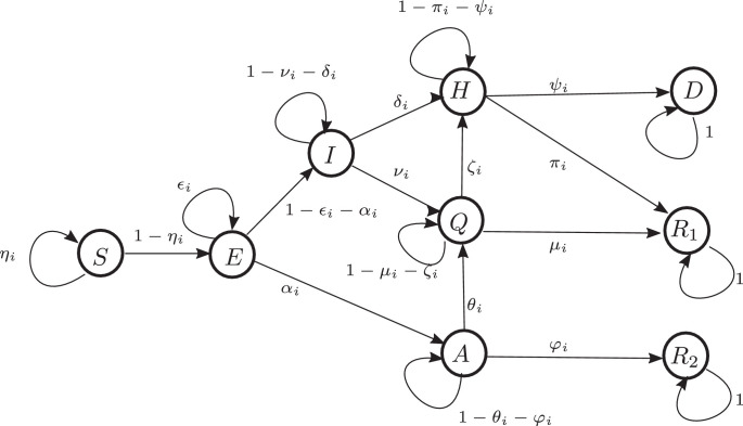
Following the line of reasoning of the contact-based discrete-time Markov-chain modeling approach for epidemic spreading in complex networks, as introduced in particular in [25] an extended susceptible-exposed-infectious-quarantine-recovered ($SEIQR$) model is derived in this section. For this purpose the infection state is separated into two classes: symptomatic (I) and asymptomatic (A). Additionally, a hospitalization state $H$, as well as a deceased state ($D$) are considered. Given that asymptomatic infections are considered there are two groups of recovered: those who were priorly identified as infected ($R_1$) and those who are not reported ($R_2$). It is supposed that an individual node can potentially infect others through a contact if it is either in the state $I$ or in the state $A$. Thus the consideration of the additional state $A$ allows to model the observed effect of hidden infectious individuals that are not directly counted by typical epidemic monitoring schemes. The resulting state transition diagram is shown in Fig. 1 and will be further discussed below.

Fig. 1.

Underlying automaton for the spreading process. At a specific time each node of the network can be in any of these states with a given probability.

The population is considered in form of a complex network of $N$ nodes represented as an undirected graph with a small–world topology [29] in which each node corresponds to a single person, a city, country of different type of group. The connection between people correspond to the links in the network. Accordingly, the adjacency matrix $A$ describing the network connections has entries

$$\begin{array}{c}\hfill a_{ij}=\{\begin{array}{cc}1,\hfill & \text{if}\text{node}i\text{and}j\text{are}\text{connected}\hfill \\ 0,\hfill & \text{else.}\hfill \end{array}\end{array}$$

Each node of the network can be in either of the 9 states. This situation is modeled by assigning a probability for each node to be in a certain state. Accordingly, denote by $s_i,e_i,p_i,q_i,h_i,a_i,r_{i1},r_{i2},d_i$ the probability of node $i\in \{1,\dots ,N\}$ to be in state $S,E,I,Q,H,A,R_1,R_2$ and $D$, respectively. A node $i$ that is susceptible will have at least one contact with its neighbor $j$ during one time step with a probability $r_{ij}$. In case that node $j$ is infected (either symptomatic or asymptomatic) such a contact goes at hand with a probability ${\beta }_i$ of contagion that is considered as a property of node $i$ only, and depends, e.g., on its immunity, mask wearing, etc.1 Accordingly, on the one side the probability of being infected during one time step through interaction with node $j$ is given by

$$a_{ij}{r}_{ij}{\beta }_i(p_j+a_j).$$

On the other side, the probability of not being infected by node $j$ is given by

$$1-a_{ij}{r}_{ij}{\beta }_i(p_j+a_j).$$

Given that all contacts are considered independent of each other, the resulting probability of not being infected during one time step is obtained by

$${\eta }_i=(1-a_{i1}{r}_{i1}{\beta }_i(p_1+a_1))\cdots (1-a_{iN}{r}_{iN}{\beta }_i(p_N+a_N))=\prod _{j=1}^N(1-a_{ij}{r}_{ij}{\beta }_i(p_j+a_j)).$$ (1)

In this way, the probability that node $i$ is infected by some neighbor during this time step is given by $1-{\eta }_i$. An infected node first passes to the incubation (or exposed) state $E$. In contrary to the transition probability from $S$ to $E$ the remaining transition probabilities are constant over time. In particular, it is supposed that a node $i$ remains in the state $E$ with a probability ${ϵ}_i$.

From $E$ there are two possible ways that the illness proceeds. With a probability ${\alpha }_i$ the node $i$ does not present symptoms and passes to the state $A$ (asymptomatic), or with a probability $1-{ϵ}_i-{\alpha }_i$ it presents symptoms and passes to the state $I$ (ill).

In both states $A$ and $I$ the node $i$ can infect other nodes by contacts, as discussed above. An infectious node in state $I$ will either pass to quarantine $\left(Q\right)$ with a probability ${\nu }_i$ or require hospitalization $\left(H\right)$ with probability ${\delta }_i$. Accordingly, the probability of staying in state $I$ is given by $1-{\nu }_i-{\delta }_i$.

A state in quarantine ($Q$) will present a positive evolution of the illness and recover, passing to the state $R_1$ with a probability ${\mu }_i$, present a negative evolution and get worse, so that it requires hospitalization with a probability ${\zeta }_i$ or remain in quarantine with a probability $1-{\mu }_i-{\zeta }_i$.

From the state of hospitalization a node can recover with probability ${\pi }_i$ and pass to the state $R_1$ or may pass away due to a very bad evolution of the illness with a probability ${\psi }_i$. Accordingly, it will remain in $H$ with probability $1-{\pi }_i-{\psi }_i$.

An asymptomatic node will pass to the state of recovery $R_2$ with a probability ${\phi }_i$ or pass to quarantine $Q$ with a probability ${\theta }_i$. The transition from $A$ to $Q$ is an important detail in the model and accounts for two possibilities: either the individual starts to present symptoms and decides to stay in quarantine, or it is detected through official tests, e.g. because it turned out to have been in contact with an officially recognized infected neighboring node. This transition probability goes at hand with the money spend into additional tests to individuals that do not present symptoms but have a significant probability of having been infected or are key hubs in the network because of a large number of contacts or high probability of contacting others. As third option, the node can remain in the state $A$ with a probability of $1-{\phi }_i-{\theta }_i$.

States in $R_1,R_2$ (recovered) and $D$ (deceased) remain there with probability 1.

The distinction between two states of recovery is made to enable a comparison with official data, given that there is no record about persons that have recovered but were asymptomatic.

To model the associated dynamics of node $i$ consider $t\in \mathbb{N}$ as a discrete time variable. Summarizing the above, for the time step between $t$ and $t+1$ one obtains

$$\begin{array}{ccc}\hfill s_i(t+1)& =& \eta \left(t\right)s_i\left(t\right)\hfill \\ \hfill e_i(t+1)& =& (1-\eta \left(t\right))s_i\left(t\right)+ϵe_i\left(t\right)\hfill \\ \hfill a_i(t+1)& =& \alpha e_i\left(t\right)+(1-\phi -\theta )a_i\left(t\right)\hfill \\ \hfill p_i(t+1)& =& (1-ϵ-\alpha )e_i\left(t\right)+(1-\nu -\delta )p_i\left(t\right)\hfill \\ \hfill q_i(t+1)& =& \nu p_i\left(t\right)+(1-\mu -\zeta )q_i\left(t\right)+\theta a_i\left(t\right)\hfill \\ \hfill h_i(t+1)& =& \delta p_i\left(t\right)+\zeta q_i\left(t\right)+(1-\pi -\psi )h_i\left(t\right)\hfill \\ \hfill r_{i1}(t+1)& =& \mu q_i\left(t\right)+\pi h_i\left(t\right)+r_{i1}\left(t\right)\hfill \\ \hfill r_{i2}(t+1)& =& \phi a_i\left(t\right)+r_{i2}\left(t\right)\hfill \\ \hfill d_i(t+1)& =& \psi h_i\left(t\right)+d_i\left(t\right)\hfill \end{array}$$ (2a)

Note that all states remain within the state-space ${[0,1]}^9$ as long as the following restrictions for the transition probabilities are satisfied (see Lemma 1 below):

$$\begin{array}{ccc}\hfill 0& \le & 1-\phi -\theta \le 1\hfill \\ \hfill 0& \le & 1-ϵ-\alpha \le 1\hfill \\ \hfill 0& \le & 1-\nu -\delta \le 1\hfill \\ \hfill 0& \le & 1-\mu -\zeta \le 1\hfill \\ \hfill 0& \le & 1-\pi -\psi \le 1\hfill \end{array}$$ (2b)

In addition to the above $9N$ difference equations for consistency the algebraic condition

$$s_i\left(t\right)+e_i\left(t\right)+p_i\left(t\right)+q_i\left(t\right)+h_i\left(t\right)+a_i\left(t\right)+r_{i1}\left(t\right)+r_{i2}\left(t\right)+d_i\left(t\right)=1$$ (2c)

must hold true for all $t\ge 0$, $i=1,\dots ,N$. In compact vector notation this can be written as a discrete-time nonlinear first-order model of the form

$$\begin{array}{ccc}& & \mathit{x}(t+1)=\mathbf{\Phi }(\mathit{x}\left(t\right),\mathit{p}),\mathit{x}\left(t\right)=\left[\begin{array}{ccc}{\mathit{x}}_1\left(t\right)& \cdots & {\mathit{x}}_N\left(t\right)\end{array}\right],\hfill \\ & & {\mathit{x}}_i\left(t\right)=\left[\begin{array}{ccc}{s}_i\left(t\right)& \cdots & d_i\left(t\right)\end{array}\right],\hfill \end{array}$$ (2d)

for $t>0$, $\mathit{x}\left(0\right)={\mathit{x}}_0$ and $i=1,\dots ,N$ with the parameter vector

$$\begin{array}{c}\hfill \mathit{p}=\left[\begin{array}{c}\beta ,ϵ,\alpha ,\varphi ,\theta ,\nu ,\delta ,\mu ,\zeta ,\pi ,\psi ,r\end{array}\right].\end{array}$$ (2e)

To identify the associated state and parameter spaces for which the model is valid introduce

$$\begin{array}{ccc}& & \mathcal{X}=\{\mathit{x}\in {[0,1]}^{9N}|\sum _{k=1}^9{x}_k=1\},\hfill \\ & & \mathcal{P}=\{\mathit{p}\in {[0,1]}^{12}|\left(2b\right)\text{holds}\text{true,}\text{with}\mathit{p}\text{given}\text{by}\left(2e\right)\}.\hfill \end{array}$$

In the following the solution vector at time $t\ge 0$ starting at ${\mathit{x}}_0$ at $t=0$ with the parameter vector $\mathit{p}$ is denoted by $\mathit{x}\left(t\right)=\mathit{x}(t;{\mathit{x}}_0,\mathit{p})$.

The following basic result presents an intrinsic and essential property of the model (2).

Lemma 1

Consider the model (2) and let$\mathit{p}\in \mathcal{P}$. Then the set$\mathcal{X}$is positively invariant, i.e., for all${\mathit{x}}_0\in \mathcal{X}$it holds true that$\mathit{x}(t;{\mathit{x}}_0,\mathit{p})\in \mathcal{X}$for all$t\ge 0$.

Proof

Consider that for some $i\in \{1,\dots ,N\}$ some state value $x_{i,k}$, $k\in \{1,\dots ,9\}$ is zero at time $t\ge 0$ and all other are greater or equal to zero, i.e. $x_{i,k}\left(t\right)=0,x_{i,l}\left(t\right)\ge 0$, $k,l\in \{1,\dots ,9\}$ and let $\mathit{p}\in \mathcal{P}$, so that the constraints (2b) hold true. It can be directly seen from (2), that $x_{i,k}(t+1)\ge 0$, given that all other states satisfy $x_{i,k}\left(t\right)\ge 0$ and the parameters satisfy the constraints (2b). This shows that for all $i=1,\dots ,9N$ it holds true that $x_{i,k}\left(t\right)\ge 0$ for all $k=1,\dots ,9$ and $t>0$ as long as $x_{i,k}\left(0\right)\ge 0$. Further, let (2c) hold true for some $t\ge 0$. A simple calculation shows that

$$\begin{array}{ccc}& & s_i(t+1)+e_i(t+1)+p_i(t+1)+q_i(t+1)+h_i(t+1)\hfill \\ & & +a_i(t+1)+r_{i1}(t+1)+r_{i2}(t+1)+d_i(t+1)\hfill \\ & & =s_i\left(t\right)+e_i\left(t\right)+p_i\left(t\right)+q_i\left(t\right)+h_i\left(t\right)+a_i\left(t\right)+r_{i1}\left(t\right)\hfill \\ & & +r_{i2}\left(t\right)+d_i\left(t\right)=1\hfill \end{array}$$

is always ensured. In consequence, the constraint (2c) is satisfied for all $t\ge 0$ if it is for $t=0$. As it also holds true that for all $i=1,\dots ,9N$ one has $0\le x_{i,k}\left(t\right)$ for all $k=1,\dots ,9$ and $t\ge 0$ it follows that $x_{i,k}\left(t\right)\le 1$. Thus $\mathit{x}\left(0\right)\in \mathcal{X}$ implies that $\mathit{x}\left(t\right)\in \mathcal{X}$ for all $t\ge 0$, i.e., $\mathcal{X}$ is positively invariant. □

Note that even though the model (2) is probabilistic in nature, given that the states indicate the probability of a node $i$ to be in one of the 9 possible states, it has a strong deterministic component as it considers only known effects and no stochastic influences. In particular this implies that the model corresponds to a closed system with no interaction with the surrounding. Furthermore, the parameters are considered homogeneous over the network, i.e. all nodes have the same transition probability up to the probability of not getting infected ${\eta }_i$, which depends on the network structure and thus mainly on the node degree.

For real spreading processes these assumptions are quite unnatural. There are several ways of getting rid of these strong assumptions. One way is to introduce different parameters satisfying a certain distribution, considering segmentation of the population in different groups, or taking into account stochasticity by means of additional stochastic inputs.

Given that official data is available only for the total number of infected, hospitalized, recovered people as well as the deceased ones, it makes sense to additionally consider the mean value model associated to the statistical sample of the network. This is addressed in the next section.

3. Model evaluation

In order to evaluate the model, official data in form of time series of reported cases in specific countries have been used that are provided by the John Hopkins University through the github site https://github.com/CSSEGISandData/COVID-19/tree/master/csse_covid_19_data/csse_covid_19_time_series. This data covers the cumulative numbers of confirmed cases $n_c$, officially recovered cases $n_{r_1}$ and deceased $n_d$ for each country.

In combination with the total number of inhabitants $n_0$ of the respective countries, this data can be used to determine the statistical probability of being confirmed, recovered, or deceased, when selecting an arbitrary group member, according to

$$y_c=\frac{n_c}{n_0},y_{r_1}=\frac{n_{r_1}}{n_0},y_d=\frac{n_d}{n_0}.$$ (3a)

These are referred to as measurements from now onwards. Recalling the state automaton shown in Fig. 1 and accounted for in model (2) it holds that the accumulative number $n_c$ is given by

$$n_c=n_q+n_h+n_{r_1}+n_d,$$

with $n_q,n_h$ being the number of people officially in quarantine and in hospital due to the infection, respectively. In accordance, a fourth indirect (i.e., model-specific) measurement is at hand, namely

$$y_{q+h}=y_c-y_d-y_{r_1}=\frac{n_q+n_h}{n_0}.$$ (3b)

This yields a measurement vector of four independent values at time $t\ge 0$

$$\begin{array}{c}\hfill \mathit{y}\left(t\right)=\left[\begin{array}{c}{y}_c\left(t\right)\\ y_{r1}\left(t\right)\\ y_d\left(t\right)\\ y_{q+h}\left(t\right)\end{array}\right].\end{array}$$ (3c)

Introducing the first moments of the state distribution over the network according to

$$\begin{array}{ccc}& & {\rho }_s\left(t\right)=\frac{1}{N}\sum _{n=1}^N{s}_n\left(t\right),{\rho }_e\left(t\right)=\frac{1}{N}\sum _{n=1}^N{e}_n\left(t\right),\hfill \\ & & {\rho }_a\left(t\right)=\frac{1}{N}\sum _{n=1}^N{a}_n\left(t\right),{\rho }_p\left(t\right)=\frac{1}{N}\sum _{n=1}^N{p}_n\left(t\right),\hfill \\ & & {\rho }_q\left(t\right)=\frac{1}{N}\sum _{n=1}^N{q}_n\left(t\right),{\rho }_h\left(t\right)=\frac{1}{N}\sum _{n=1}^N{h}_n\left(t\right),\hfill \\ & & {\rho }_{r1}\left(t\right)=\frac{1}{N}\sum _{n=1}^N{r}_{n1}\left(t\right),{\rho }_{r2}\left(t\right)=\frac{1}{N}\sum _{n=1}^N{r}_{n2}\left(t\right),\hfill \\ & & {\rho }_d\left(t\right)=\frac{1}{N}\sum _{n=1}^N{d}_n\left(t\right)\hfill \end{array}$$ (4)

$$\begin{array}{ccc}\hfill \mathit{\rho }\left(t\right)& =& {\left[\begin{array}{c}{\rho }_s\left(t\right){\rho }_e\left(t\right){\rho }_a\left(t\right){\rho }_p\left(t\right){\rho }_q\left(t\right){\rho }_h\left(t\right){\rho }_{r_1}\left(t\right){\rho }_{r_2}\left(t\right){\rho }_d\left(t\right)\end{array}\right]}^{\top }\hfill \\ & =& \frac{1}{N}\sum _{n=1}^N{\mathit{x}}_n\left(t\right),\hfill \end{array}$$ (5)

one can obtain a model-based representation of the measured data $\mathit{y}\left(t\right)$ given in (3c) in the form

$$\mathit{y}\left(t\right)=H\mathit{x}\left(t\right)=C\mathit{\rho }\left(t\right)$$ (6)

with the matrixes

$$\begin{array}{ccc}& & C:=\left[\begin{array}{c}{\mathit{c}}_1^{\top }\\ ⋮\\ {\mathit{c}}_4^{\top }\end{array}\right]=\left[\begin{array}{ccccccccc}0& 0& 0& 0& 1& 1& 1& 0& 1\\ 0& 0& 0& 0& 0& 0& 1& 0& 0\\ 0& 0& 0& 0& 0& 0& 0& 0& 1\\ 0& 0& 0& 0& 1& 1& 0& 0& 0\end{array}\right],\hfill \\ & & \text{rank}\left(C\right)=4,H=I_N\otimes C\hfill \end{array}$$ (7)

with the $N\times N$ identity matrix $I_N$. For a given data set $\{\mathit{y}\left(t_s\right),\mathit{y}\left(t_f\right)\}$ of time series with $0\le t_s<t_f$ consisting of data points at successive time instances $t_s=t_1\le t_2\le \dots \le t_{nm}=t_f$, the parameter estimation problem can be addressed e.g. using a robust weighted least squares approach [4]

$$\begin{array}{cc}& \underset{\mathit{p},{\mathit{x}}_0}{\min }\sum _{\tau =t_s}^{t_f}\sum _{k=1}^4{w}_k\left(\tau \right)\mathcal{L}\left({(y_k\left(\tau \right)-{\mathit{c}}_k^{\top }\mathit{\rho }(\tau ;t_s,\mathit{p},{\mathit{x}}_0))}^2\right)\hfill \\ \hfill & \text{subject}\text{to}\mathit{p}\in \mathcal{P},{\mathit{x}}_0\in \mathcal{X}\hfill \end{array}$$ (8)

with the solution of (2d) starting at time $t_s$ with the value ${\mathit{x}}_0$ and running with parameter vector $\mathit{p}$ denoted by $\mathit{x}(\tau ;t_s,\mathit{p},{\mathit{x}}_0)$, positive weights $w_k\left(t\right)>0,t\in [t_s,t_f]$, and a nonlinear function $\mathcal{L}\in {\mathcal{C}}^1({\mathbb{R}}^n,\mathbb{R})$. For the present work, motivated by [30], the sub-linear function $\mathcal{L}=\arctan$ has been employed. The reason for this choice is that for small errors a similar behavior as the one of the absolute error is obtained, implying a higher sensitivity in comparison to the classical least squares approach whilst ensuring differentiability at zero. The weights $w_k$ in (8) can be adapted, e.g., giving more influence to time intervals of high dynamic behavior.

To provide an illustrative example the data for Germany (GER), Mexico (MEX) and the United States of America (USA) have been extracted from the above database and a parameter identification has been carried out using the model (2). This choice was taken to be able to show the functioning for considerably different social, health-political and health-structural conditions.2 For the comparison a network of $N=200$ nodes has been used with a small-world structure [29], mean node degree $k=4$ and build with the Python algorithm networks.watts_strogatz_graph with a reconnection probability of $p=.4$. Note that this particular choice of network is arbitrary and just serves to illustrate the adaptation capabilities of the model, as well as the combination with model-based monitoring schemes addressed in the next section. The total numbers of inhabitants are approximated by

$$n_{0,GER}=83·{10}^6,n_{0,MEX}=126.2·{10}^6,n_{0,USA}=328.2·{10}^6.$$

As initial guess for the model parameter vector $\mathit{p}$ the characteristic transient times and associated probabilities of staying in a certain state of the automaton (see Fig. 1) provided by the Robert Koch institute in Germany [31] [available at https://www.rki.de/DE/Content/InfAZ/N/Neuartiges_Coronavirus/Modellierung_Deutschland.html (page 4, in German)] have been used. To highlight the main idea behind this approach, consider that it is known that a node $i$ is in state $A$ with probability 1 at time $t$, i.e., $a_i\left(t\right)=1$. The parameters provided in the mentioned document state basically that this node will be recovered after 9 days with a probability of 95.5$\%$, i.e., $a_i(t+9)=0.045$. In terms of the above parameters, this can be interpreted as follows:

$$a_i(t+9)=0.045={(1-\varphi -\theta )}^9{a}_i\left(t\right)={(1-\varphi -\theta )}^9$$

so that

$$1-\varphi -\theta =0.{045}^{1/9}.$$

Employing similar arguments for the remaining states using the provided data and completing the missing data reasonably an initial parameter vector is obtained. The initial value ${\mathit{x}}_0$ is determined considering that only the first node with $i=1$ in the network is infectious with probability $p_1\left(t_0\right)=p_{10}$ and all other nodes are susceptible. The adaptation of the parameters within reasonable bounds contained in (0,1), satisfying the constraints (2b) and providing a solution of the mean squares minimization problem (8) is carried out using scipy.optimize.minimize in Python choosing $t_s=50,t_f=200$. The initial time is set to 50, given that we decided to keep the time step of the original database while in the considered countries there were almost no cases during the first weeks of the pandemic. This approach can be applied repetitively, varying the weights $w_k\left(t\right)$ between successive optimization runs. This yields the results shown in Figs. 2 - 4 with the parameter vectors

$$\begin{array}{ccc}\hfill {\mathit{p}}_{GER}& =& [0.06114,0.42081,0.57891,0.59280,0.07341,0.00238,\hfill \\ & & 0.00019,0.02186,0.22082,0.06842,0.00485,0.93594],\hfill \end{array}$$ (9a)

$$\begin{array}{ccc}\hfill {\mathit{p}}_{MEX}& =& [0.02623,0.87733,0.10315,0.06991,0.30881,0.00003,\hfill \\ & & 0.00072,0.10913,0.02888,0.40195,0.25909,0.45380],\hfill \end{array}$$ (9b)

$$\begin{array}{ccc}\hfill {\mathit{p}}_{USA}& =& [0.06121,0.86170,0.05789,0.90835,0.04509,0.00841,\hfill \\ & & 0.00340,0.01956,0.06165,0.00550,0.00088,0.15876].\hfill \end{array}$$ (9c)

and initial conditions $p_{10,GER}=0.68979,p_{10,MEX}=0.17363,p_{10,USA}=0.80265,p_{k0}=0,k=2,\dots ,N$.

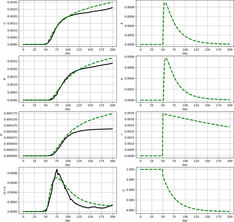
Fig. 2.

Comparison between official data and simulation results for Germany using (2) and (9a). Official data (black, solid lines) and model prediction (green, dashed lines). (For interpretation of the references to colour in this figure legend, the reader is referred to the web version of this article.)

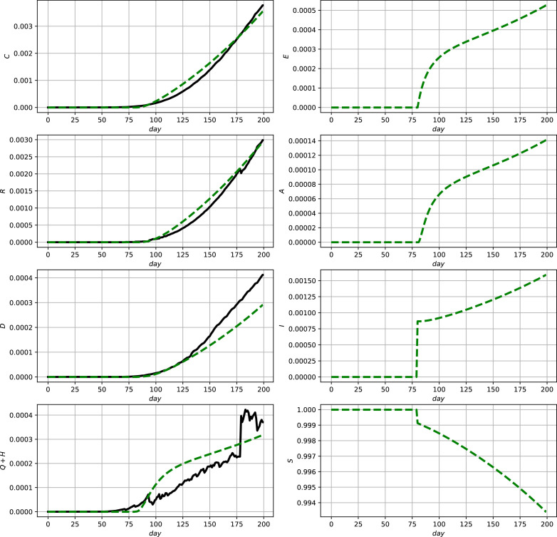
Fig. 4.

Comparison between official data and simulation results for USA using (2) and (9c). Official data (black, solid lines) and model prediction (green, dashed lines). (For interpretation of the references to colour in this figure legend, the reader is referred to the web version of this article.)

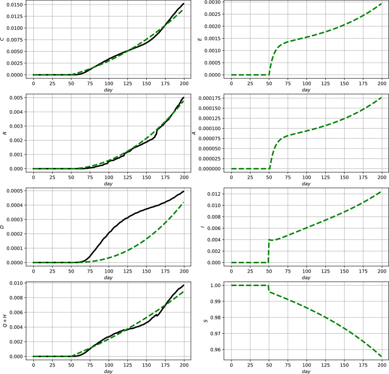
According to these simulation results the model shows a good capability to qualitatively and quantitatively describe the development of the reported numbers, i.e., the measurements. In the case of discontinous measurement data as, e.g., in Fig. 3 in the lower left subfigure, it is typical that a parameter optimization yields the shown averaging behavior. To be able to better account for such discontinuities in the next section an online data–assimilation scheme will be proposed.

Fig. 3.

Comparison between official data and simulation results for Mexico using (2) and (9b). Official data (black, solid lines) and model prediction (green, dashed lines). (For interpretation of the references to colour in this figure legend, the reader is referred to the web version of this article.)

It should be noted that even though the presented simulation results show in principle a good correspondence with the actual data, there has been only few interpretation of the parameters in the sense of further constraints which are motivated by physical-physiological or medical reasoning. Actually there exist different parameter sets for which a good correspondence with the observed data is achieved. In consequence, the presentation of the present parameters does not aim to claim that these are the most accurate ones. In particular, the optimized parameter set will always depend, e.g., on the particular network model used. Hence, the results of this section only aim to show that the model can provide adequate predictions when it is adequately parameterized.

It should be further mentioned that the nonlinearity and high-dimension of the model implies a considerable parameter sensitivity. Anyway, the strength of the model consists in the insight associated to the contact–based modeling approach. As mentioned above, the accuracy of the prediction and the correspondence with the measurements will be improved in the next section by means of a Kalman–Filter based, real–time capable state estimation scheme.

4. Stochastic state estimation for epidemic spreading

Given that spreading does normally not take place in isolated populations and that parameters vary over time, e.g., due to an increase in contact limitations, increased wearing of masks, vaccination, etc., one has to account for unmodeled time varying effects influencing the dynamics of the underlying process. One way of addressing such fluctuations consists in including stochastic variations in the process model in form of additive white noise yielding

$$\mathit{x}(t+1)=\mathbf{\Phi }\left(\mathit{x}\right(t),\mathit{p})+\mathit{w}\left(t\right),t>0,\mathit{w}\sim \mathcal{N}(\mathit{0},Q)$$ (10a)

$$\mathit{y}\left(t\right)=H\mathit{x}\left(t\right)+\mathit{v}\left(t\right),\mathit{v}\sim \mathcal{N}(\mathit{0},R)$$ (10b)

with normally distributed initial state $\mathit{x}\left(t_0\right)\sim \mathcal{N}({\mathit{x}}_0,Q_0)$ and state and measurement covariance matrices $Q_0,Q,R\succ 0$. Note that this is the most simple form to account for unmodeled effects. The noise could also enter the dynamics with state dependent covariance, leading to so-called multiplicative noise [32], [33], [34]. It is know from different studies, that additive and multiplicative noise has quite different effects, in particular for the time evolution of the mean and mode of the associated probability distributions [32], [34]. For the purpose of illustrating the monitoring methodology addressed in this work the setup with additive noise is sufficient and yields sufficiently convincing results.

For monitoring purposes it is important to have information about the unmeasured states. Besides the statistically relevant mean densities ${\rho }_s,{\rho }_e,{\rho }_a,{\rho }_q,{\rho }_h,{\rho }_{r_2}$, the approach presented in the sequel actually provides information down to the lowest level, i.e., the state probabilities of each node in the network. In particular this includes information about the number of asymptomatic groups. This information can be obtained in form of a state estimate $\widehat{\mathit{x}}\left(t\right)$ at time $t\ge 0$ that is provided by an estimation scheme which takes into account the stochastic model (10), i.e., the underlying process mechanisms together with the statistics coded in the covariances, in combination with the existing measurement updates, i.e., the daily new reported data vector $\mathit{y}\left(t\right)$. Typical approaches for such a task are known from systems and control theory and named observers or filters [14]. Given the intrinsic probabilistic nature of the uncertainties the Kalman Filter approaches seem suitable [14], [15], [35] and have already been exploited for simpler models for COVID-19 supervision [9], [10], [11], [22] without considering structural details of the underyling networks. The Kalman Filter provides a minimum state estimation error covariance, thus providing an optimal estimate of unmeasured states by combining the model prediction with the innovation based on the comparison with the updated measurements. For nonlinear systems, the extended Kalman Filter can be employed, which provides a local Gaussian approximation of the probability distribution along the estimated state trajectory [14]. It is also known, that, from a non local perspective, this approximation can potentially be misleading for nonlinear systems [15], [35].

Both, the classical and extended Kalman Filters require the explicit calculation of the time varying covariance matrices. Note that due to the typically high-dimensional dynamics of the presented model with $9N$ states, where $N$ is the number of nodes in the network, and the inherent nonlinear behavior, approaches based on the (classical or extended) Kalman Filter seem rather inappropriate for the case at hand. In contrast to the mentioned monitoring schemes, the ensemble Kalman Filter (enKF) is based on a Markov Chain Monte Carlo simulation with data assimilation (state innovation) by measurement injection [15], [35]. The basic idea consists in employing $M$ different simultaneous simulations of the process for predictions ${\widehat{\mathit{x}}}_p^k$, $k=1,\dots ,M$ and using the sample mean and covariances instead of the explicit calculation of the covariance dynamics.

The enKF is implemented as follows [14], [35]:

Given the estimated state $\widehat{\mathit{x}}(t-1)$ at time $t-1$, the following steps are carried out:

• •
  Prediction (model–based without using the actual measurements):

  $${\widehat{\mathit{x}}}_p\left(t\right)=\mathbf{\Phi }(\widehat{\mathit{x}}(t-1),\mathit{p})+\mathit{w},t\ge 1,\widehat{\mathit{x}}\left(t_0\right)={\widehat{\mathit{x}}}_0,\mathit{w}\sim \mathcal{N}(\mathit{0},Q)$$ (11a)

  with ${\widehat{\mathit{x}}}_p\left(t\right)={[{\widehat{\mathit{x}}}_{p,1}\left(t\right),\cdots ,{\widehat{\mathit{x}}}_{p,N}\left(t\right)]}^{\top }$
• •
  Determination of the prediction covariance and Kalman (correction) gain:

  $$P\left(t\right)=\frac{1}{N-1}\sum _{n=1}^N{({\widehat{\mathit{x}}}_n-〈{\widehat{\mathit{x}}}_p\left(t\right)〉)}^2,〈{\widehat{\mathit{x}}}_p\left(t\right)〉=\frac{1}{N}\sum _{n=1}^N{\widehat{\mathit{x}}}_{k,p}\left(t\right)$$ (11b)

  $$K\left(t\right)=P\left(t\right)H^{\top }{(HP\left(t\right)H^{\top }+R)}^{-1},$$ (11c)
• •
  Data assimilation (innovation by means of measurement–driven correction of the predicted values):

  $$\widehat{\mathit{x}}\left(t\right)=(I-K(t\left)H\right){\widehat{\mathit{x}}}_p\left(t\right)+K\left(t\right)\mathit{y}\left(t\right)$$ (11d)

  $$\widehat{\mathit{\rho }}\left(t\right)=〈\widehat{\mathit{x}}\left(t\right)〉=\frac{1}{N}\sum _{n=1}^N{\widehat{\mathit{x}}}_k\left(t\right)$$ (11e)

For the numerical evaluation of the ensemble Kalman Filter the parameter vectors provided in (9) are used, the covariance matrices $Q,R$ are set as

$$\begin{array}{cc}\hfill Q& =\text{diag}\left([2·{10}^{-10},2·{10}^{-10},{10}^{-14},{10}^{-14},{10}^{-14},{10}^{-10},{10}^{-15}]\right),\hfill \\ \hfill R& =\text{diag}\left([{10}^{-20},{10}^{-21},{10}^{-20},{10}^{-21}]\right)\hfill \end{array}$$

and an initial distribution over the ensemble with mean $p_{10,X}$ from the parameter identification with $X\in \{$GER, MEX, USA$\}$, and variance $q_0={10}^{-18}$ is considered. The evaluation is carried out over the time interval $t_0=50$ to $t_f=323$, i.e. 123 days more than used to fit the initial parameter set with the results shown in Figs. 2–4.

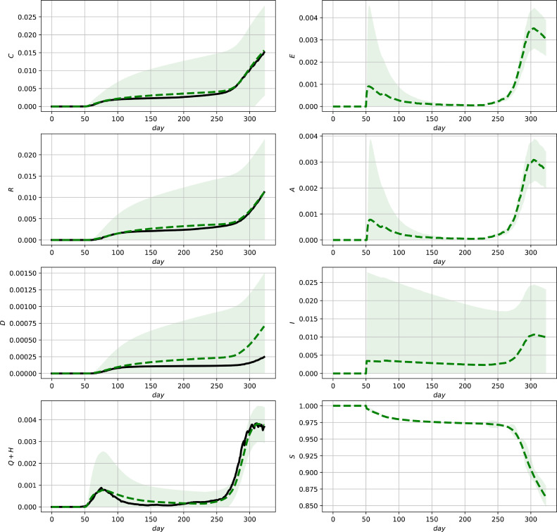
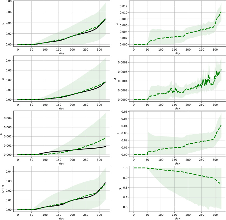
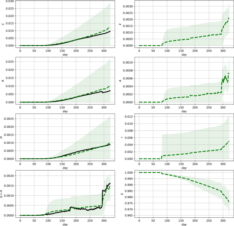
The results are illustrated in Figs. 5 - 7 showing the state estimates with variance-band ($\sigma /2$) confidence intervals together with the measurements (3c). It can be seen that the resulting state estimates show a good correspondence with the measurements and additionally provide model-based (and thus parameter dependent) estimates of the unmeasured states which can be further used for diagnosis or decisions for action plans. The different shapes of the confidence intervals illustrate their different nonlinear interdependencies on the state estimates as well as the measurements due to the innovation step (11e). The improvement in comparison to the model predictions shown in Figs. 2–4 can be most clearly seen in the case of Mexico, where discontinuities in the measurements are present (see, e.g., the lower left subfigure in 3 and 6 ). The final deviations in the predictions of the fraction of deceased group members for Germany and the US reveal that a reparameterization after 200 time units would be required to improve the model fit. As infection parameters, as well as medical treatment varies over time, such a reparameterization would be a necessary improvement for the use in the long run. This applies in particular for taking into account vaccinations which did not play a central rule during the phase of the pandemic shown in the figures.

Fig. 5.

Evaluation of the ensemble Kalman Filter for the complete data set for Germany. Official data (black, solid lines) and predictions (green, dashed lines) and ($\sigma /2$) confidence intervals (green shaded regions). (For interpretation of the references to colour in this figure legend, the reader is referred to the web version of this article.)

Fig. 7.

Evaluation of the ensemble Kalman Filter for the complete data set for the USA. Official data (black, solid lines) and predictions (green, dashed lines) and ($\sigma /2$) confidence intervals (green shaded regions). (For interpretation of the references to colour in this figure legend, the reader is referred to the web version of this article.)

Fig. 6.

Evaluation of the ensemble Kalman Filter for the complete data set for Mexico. Official data (black, solid lines) and predictions (green, dashed lines) and ($\sigma /2$) confidence intervals (green shaded regions). (For interpretation of the references to colour in this figure legend, the reader is referred to the web version of this article.)

5. Discussion

As commented at the end of Section 3, the purpose of the present paper consists in presenting a new model which is capable to allow online monitoring using a model-based data assimilation and state estimation scheme. The contribution is thus overall of methodological nature. In order to adapt the model and approach further for specific usage, the following measures can be considered:

• •Combination of the approach with online parameter adaptation schemes. As the parameters often vary over larger time intervals (see also the final discussion in the previous section), e.g., due to different countermeasures in different moments, such an adaptation could improve the estimation performance and enrich the usability of the proposed approach. For this purpose one can either consider a reparametrization over a receding horizon, i.e., taking into account the last $k$ days, using either the presented approach, a moving horizon estimation technique [36], or include some of the parameters in the state vector with a stochastic variation and adaptation by measurement injection approach.
• •Stratification of the population, i.e., considering, e.g., more vulnerable groups with higher infection probabilities $\beta$, or higher probability of being asymptomatic, i.e., with larger $\alpha$. Such an approach would enable to study in more detail the different consequences of parameter diversity. On the one side this can provide additional inside into the spreading process, but on the other side also implies a substantial blow-up in the number of parameters to be identified. Thus, particular local (i.e., on the basis of sub-networks) identification schemes should be employed for such a task.
• •Consideration of local geographical, transport or travelling networks or individual network data evaluated from mobile phones, analysis of interchange between cities, regions or countries. With such information further understanding the mutual influence and designing corresponding counter-measures would be explicitly possible.

6. Conclusions

In this paper a contact–based Markov chain model for the spread of a virus in a complex network has been presented that particularly takes into account the asymptomatic group. The ability of the model to fit with actual data over long term horizons has been illustrated for three completely different case studies, namely Germany, Mexico and the U.S.A. The potential of adequately using such models for data assimilation and reconstruction of hidden states has been shown using the ensemble Kalman Filter. The results show that this framework provides an efficient means that can be further exploited using more detailed insight about the underlying contact network structure and parameters. The long-term estimation model presented by the authors shows the fruitful combination of contact-based network spreading models with a modern state estimation and filtering technique to (i) enable real-time monitoring and (ii) efficiently deal with dimensionality and stochastic uncertainties. Having such monitoring schemes, capable of fast adaptation to new parametric scenarios can provide an additional basis for further decision making processes.

CRediT authorship contribution statement

A. Schaum: Conceptualization, Methodology, Software, Formal analysis, Investigation, Writing – original draft, Writing – review & editing, Visualization, Project administration. R. Bernal-Jaquez: Conceptualization, Methodology, Writing – original draft, Investigation, Writing – review & editing, Visualization, Project administration. L. Alarcon Ramos: Methodology, Software, Formal analysis, Resources, Investigation, Writing – original draft, Writing – review & editing.

Declaration of Competing Interest

The authors declare that they have no known competing financial interests or personal relationships that could have appeared to influence the work reported in this paper.

References

- 1.Estrada E. COVID-19 and SARS-CoV-2. Modeling the present, looking at the future. Phys Rep. 2020;869:1–51. doi: 10.1016/j.physrep.2020.07.005. [DOI] [PMC free article] [PubMed] [Google Scholar]
- 2.Nowzari C., Preciado V.M., Pappas G.J. Analysis and control of epidemics: a survey of spreading processes on complex networks. IEEE Control Syst. 2016;36(1):26–46. doi: 10.1109/MCS.2015.2495000. [DOI] [Google Scholar]
- 3.Schurwanz M., Höher P.A., Bhattacharjee S., Damrath M., Stratmann L., Dressler F. Infectious disease transmission via aerosol propagation from a molecular communication perspective: shannon meets coronavirus. arXiv. 2020 [Google Scholar]
- 4.Ljung L. Prentice Hall, New Jersey; 1987. System identification: theory for the user. [Google Scholar]
- 5.Alakus T.B., Turkoglu I. Comparison of deep learning approaches to predict COVID-19 infection. Chaos Soliton Fract. 2020;140:110120. doi: 10.1016/j.chaos.2020.110120. [DOI] [PMC free article] [PubMed] [Google Scholar]
- 6.Zeroual A., Harrou F., Dairi A., Sun Y. Deep learning methods for forecasting COVID-19 time-series data: a comparative study. Chaos Soliton Fract. 2020;140:110121. doi: 10.1016/j.chaos.2020.110121. [DOI] [PMC free article] [PubMed] [Google Scholar]
- 7.Shastri S., Singh K., Kumar S., Kour P., Mansotra V. Time series forecasting of covid-19 using deep learning models: india-usa comparative case study. Chaos Soliton Fract. 2020;140:110227. doi: 10.1016/j.chaos.2020.110227. [DOI] [PMC free article] [PubMed] [Google Scholar]
- 8.Shahid F., Zameer A., Muneeb M. Predictions for COVID-19 with deep learning models of lstm, gru and bi-lstm. Chaos Soliton Fract. 2020;140:110212. doi: 10.1016/j.chaos.2020.110212. [DOI] [PMC free article] [PubMed] [Google Scholar]
- 9.Singh K.K., Kumar S., Dixit P., Bajpai M.K. Kalman filter based short term prediction model for COVID-19 spread. Appl Intell. 2020 doi: 10.1007/s10489-020-01948-1. [DOI] [PMC free article] [PubMed] [Google Scholar]
- 10.Zeng X., Ghanem R. Dynamics identification and forecasting of COVID-19 by switching kalman filters. Comput Mech. 2020;66:1179–1193. doi: 10.1007/s00466-020-01911-4. [DOI] [PMC free article] [PubMed] [Google Scholar]
- 11.Aslam M. Using the kalman filter with arima for the COVID-19 pandemic dataset of pakistan. Data Brief. 2020;31:105854. doi: 10.1016/j.dib.2020.105854. [DOI] [PMC free article] [PubMed] [Google Scholar]
- 12.Maleki M., Mahmoudi M.R., Heydari M.H., Pho K.-H. Modeling and forecasting the spread and death rate of coronavirus (covid-19) in the world using time series models. Chaos Soliton Fract. 2020;140:110151. doi: 10.1016/j.chaos.2020.110151. [DOI] [PMC free article] [PubMed] [Google Scholar]
- 13.De Simone A., Piangerelli M. A bayesian approach for monitoring epidemics in presence of undetected cases. Chaos Soliton Fract. 2020;140:110167. doi: 10.1016/j.chaos.2020.110167. [DOI] [PMC free article] [PubMed] [Google Scholar]
- 14.Gelb A. M.I.T. Press, Cambridge; 1978. Applied optimal estimation. [Google Scholar]
- 15.Evensen G. 2nd. Springer-Verlag Berlin Heidelberg; 2009. Data assimilation: the ensemble kalman filter. [Google Scholar]
- 16.Kermack W.O., McKendrick A.G. A contribution to the mathematical theory of epidemics. Proc Royal Soc. 1927;A(115):700. doi: 10.1007/BF02464423. [DOI] [PubMed] [Google Scholar]
- 17.Pastor-Satorras R., Castellano C., Van Mieghem P., Vespignani A. Epidemic processes in complex networks. Rev Mod Phys. 2015;87:925–979. doi: 10.1103/RevModPhys.87.925. [DOI] [Google Scholar]
- 18.Nkwayep C.H., Bowong S., Tewa J., Kurths J. Short-term forecasts of the COVID-19 pandemic: a study case of cameroon. Chaos Soliton Fract. 2020;140:110106. doi: 10.1016/j.chaos.2020.110106. [DOI] [PMC free article] [PubMed] [Google Scholar]
- 19.Avila-Ponce de León U., Ángel G.C. Pérez, Avila-Vales E. An seiard epidemic model for COVID-19 in mexico: mathematical analysis and state-level forecast. Chaos Soliton Fract. 2020;140:110165. doi: 10.1016/j.chaos.2020.110165. [DOI] [PMC free article] [PubMed] [Google Scholar]
- 20.Humphries R., Spillane M., Mulchrone K., Wieczorek S., O’Riordain M., Hövel P. A metapopulation network model for the spreading of SARS-CoV-2: case study for ireland. Infectious Disease Modelling. 2021;6:420–437. doi: 10.1016/j.idm.2021.01.004. [DOI] [PMC free article] [PubMed] [Google Scholar]
- 21.Nabi K.N. Forecasting COVID-19 pandemic: a data-driven analysis. Chaos Soliton Fract. 2020;139:110046. doi: 10.1016/j.chaos.2020.110046. [DOI] [PMC free article] [PubMed] [Google Scholar]
- 22.Hasan A., Putri E.R.M., Susanto H., Nuraini N. Data-driven modeling and forecasting of covid-19 outbreak for public policy making. ISA Trans. 2021;In press doi: 10.1016/j.isatra.2021.01.028. [DOI] [PMC free article] [PubMed] [Google Scholar]
- 23.Kremer R.. Using Kalman filter to predict coronavirus spread. https://towardsdatascience.com/using-kalman-filter-to-predict-corona-virus-spread-72d91b74cc8; 2020a.
- 24.Kremer R.. Coronavirus spread prediction. https://medium.com/analytics-vidhya/coronavirus-updated-prediction-using-kalman-filter-3ef8b7a72409, Accessed March, 4, 2021; 2020b.
- 25.Gómez S., Arenas A., Borge-Holthoefer J., Meloni S., Moreno Y. Discrete-time markov chain approach to contact-based disease spreading in complex networks. EPL (Europhysics Letters) 2010;89(3):38009. [Google Scholar]
- 26.Alarcón-Ramos L.A., Bernal Jaquez R., Schaum A. Output-feedback control of virus spreading in complex networks with quarantine. Front Appl Math Stat. 2018;4:34. doi: 10.3389/fams.2018.00034. [DOI] [Google Scholar]
- 27.Basnarkov L. Seair epidemic spreading model of covid-19. Chaos Soliton Fract. 2021;142:110394. doi: 10.1016/j.chaos.2020.110394. [DOI] [PMC free article] [PubMed] [Google Scholar]
- 28.Schaum A., Jaquez R.B. Estimating the state probability distribution for epidemic spreading in complex networks. Appl Math Comput. 2016;291:197–206. doi: 10.1016/j.amc.2016.06.037. [DOI] [Google Scholar]
- 29.Watts D., Strogatz S. Collective dynamics of “small-world” networks. Nature. 1998;393:440–442. doi: 10.1038/30918. [DOI] [PubMed] [Google Scholar]
- 30.Triggs B., McLauchlan P., Hartley R.I., Fitzgibbon A. In: Vision Algorithms: Theory and Practice. IWVA 1999. Triggs B., Zisserman A., Szeliski R., editors. vol. 1883. Springer, Berlin, Heidelberg; 2000. Bundle adjustment - a modern synthesis. (Lecture Notes in Computer Science). [DOI] [Google Scholar]
- 31.an der Heiden M., Buchholz U. Modellierung von Beispielszenarien der SARS-CoV-2-Epidemie 2020 in Deutschland. 2020 doi: 10.25646/6571.2. [DOI] [Google Scholar]
- 32.Jazwinski A.H. Academic Press, New York; 1970. Stochastic processes and filtering theory. [Google Scholar]
- 33.Gardiner C. Springer-Verlab Berlin Heidelberg; 2009. Stochastic methods: A Handbook for the natural and social sciences. [Google Scholar]
- 34.Horsthemke W., Lefever R. Springer-Verlab Berlin Heidelberg; 1984. Noise-Induced transitions: theory and applications in physics, chemistry, and biology. [Google Scholar]
- 35.Evensen G. The ensemble kalman filter: theoretical formulation and practical implementation. Ocean Dyn. 2003;53:343–367. [Google Scholar]
- 36.Ji L., Rawlings J.B., Hu W., Wynn A., Diehl M. Robust stability of moving horizon estimation under bounded disturbances. IEEE Trans Autom Control. 2016;61(11):3509–3514. [Google Scholar]