SCAN-IT: Domain segmentation of spatial transcriptomics images by graph neural network

Abstract

Complex biological tissues consist of numerous cells in a highly coordinated manner and carry out various biological functions. Therefore, segmenting a tissue into spatial and functional domains is critically important for understanding and controlling the biological functions. The emerging spatial transcriptomics technologies allow simultaneous measurements of thousands of genes with precise spatial information, providing an unprecedented opportunity for dissecting biological tissues. However, how to utilize such noisy, sparse, and high dimensional data for tissue segmentation remains a major challenge. Here, we develop a deep learning-based method, named SCAN-IT by transforming the spatial domain identification problem into an image segmentation problem, with cells mimicking pixels and expression values of genes within a cell representing the color channels. Specifically, SCAN-IT relies on geometric modeling, graph neural networks, and an informatics approach, DeepGraphInfomax. We demonstrate that SCAN-IT can handle datasets from a wide range of spatial transcriptomics techniques, including the ones with high spatial resolution but low gene coverage as well as those with low spatial resolution but high gene coverage. We show that SCAN-IT outperforms state-of-the-art methods using a benchmark dataset with ground truth domain annotations.

1. Introduction

Complex tissues in multicellular organisms consist of numerous highly coordinated cells to carry out essential functions that vary botspatially and temporally to maintain their structures and functions. Cellular heterogeneity in different spatial contexts provides diverse biological functions and cells in a spatial domain often organize their compositions to achieve unique functions. The correct identification of spatial domains is the foundation of down-stream tasks such as reliable assessment of disease progression. Previously, identifying such spatial domain requires anatomical experiments and known markers to specify regions that are often challenging and non-scalable.

The recent spatial transcriptomics (ST) technologies [5, 14, 16] can produce spatial images of many genes simultaneously at the resolution of individual cells or a small group of cells. Such emerging datasets provide unprecedented opportunities to dissect spatial domains without using prior knowledge of the spatial domain marker genes (genes that are highly expressed within the domain but lowly expressed elsewhere). Here, we transform such spatial domain identification problem into a classic image segmentation problem, where cells are treated as pixels in an image and gene expressions within cells represent different channels (analogous to RGB channels) [12]. One major difference and a challenge, however, is the number of channels, which is significantly larger in ST data compared to classical images with three channels. In addition, the signal detection in current ST technologies is often noisy and sparse, leaving segmentation more difficult.

Reducing the number of channels by using only spatially-variable genes instead of highly-variable genes without spatial constraints can improve the tissue segmentation [10]. Preprocessing procedures, such as smoothing gene expression in space, can also lead to improved tissue domain annotations [13]. Another approach is to incorporate spatial constraints in the classical clustering methods to make cells “spatially-aware”. For example, SmfishHmrf constructs a hidden random Markov field model on the cell proximity graph by including the gene expression dependency between cells [21], and BayesSpace uses a Bayesian model to make spatially neighboring cells more likely to be in the same cluster [20]. These methods, however, are based on prescribed and simplified probabilistic models, resulting in limited applicability.

Here we utilize the deep graph neural networks method for tissue segmentation by translating it into a clustering-based image segmentation problem. This interpretation will treat ST data as an image with irregular grids and thousands of channels. To identify tissue domains in an unbiased manner from such an image, we propose a deep learning method, named SCAN-IT. Specifically, SCAN-IT first builds a geometry-aware spatial proximity graph with the nodes as the spots (a group of cells) or individual cells in ST data using alpha complex. Compared to commonly used k-nearest neighbor graphs, this graph representation better captures the physical proximity among cells. We adapt Deep Graph Infomax [17] to generate low-dimensional embeddings of the nodes. These embeddings represent both gene expression patterns in the cells and the gene expression patterns in their microenvironment by preserving the neighborhood information through the intrinsic property of DeepGraphInfomax. Finally, the resultant low-dimensional representation is fed to commonly used clustering algorithms to derive the tissue domains. We evaluate SCAN-IT both qualitatively on several ST data with various spatial resolutions, and quantitatively, on a benchmark dataset with ground-truth. In the quantitative benchmark, SCAN-IT outperforms other existing methods [10, 13, 20, 21]. SCAN-IT software is available at github.com/zcang/SCAN-IT.

2. Method

2.1. Spatial transcriptomics image segmentation problem

A ST dataset can be regarded as a 2-dimensional point cloud of N_S points (spots). On each spot, the expression of N_G genes are measured assembling a feature vector. Therefore, a ST dataset is often represented by a position matrix $P\in {ℝ}^{N_S\times 2}$ and a gene expression matrix ${ℝ}_{+}^{N_S\times N_G}$ of the spots. The purpose of domain segmentation of ST data is to separate the N_S spots into clusters (spatial regions) that are homogeneous within a cluster and differ between clusters in terms of gene expressions. This task is analogous to the image segmentation task except two main differences: 1) the ST data are represented by irregular point clouds in space and 2) there are thousands of channels (genes) in ST data compared to the three color channels in images.

2.2. Determining spatial adjacency by alpha complex

A graph of the spatial spots of cells is constructed by using alpha complex. A Voronoi cell is first constructed for each spot located at r as

$$V\left(\mathbf{\text{r}}\right)=\left\{\mathbf{\text{x}}\in {ℝ}^2|‖\mathbf{\text{x}}-\mathbf{\text{r}}‖\le ‖\mathbf{\text{x}}-{\mathbf{\text{r}}}^{\prime }‖,\forall {\mathbf{\text{r}}}^{\prime }\in P\right\},$$ (1)

where P is the set of locations for the spatial spots and ǁ·ǁ is 2-norm. Then we use the 1-skeleton of the alpha complex [4] to derive the neighborhood graph of the spots in ST data as G_α (P, δ ) = (V, E) with edges defined as

$$E=\left\{\left(i,j\right)|{\cap }_{k\in \left\{i,j\right\}}\left(V\left({\mathbf{\text{r}}}_k\right)\cap B\left({\mathbf{\text{r}}}_k,\delta \right)\right)\ne \cancel{0}\right\},$$ (2)

where B(x, δ ) is a closed ball in ${ℝ}^2$ centered at x with a radius δ. The radius δ is estimated by the average distance of the spots to their k nearest neighbors.

2.3. Graph convolutional network as the encoder

To derive a low-dimensional node representation that encode gene expression patterns both on the node and its microenvironment, an encoder that has the potential to characterize spatial neighborhood information is needed. To this end, we use a graph convolutional network (GCN) [8] to derive low-dimensional representations of the spots in ST data. When applied to image segmentation, GCN has the advantage of better preserving segment boundaries [15] compared with deep convolutional neural networks. Given a data with N_S spots from which an adjacency matrix $A\in {ℝ}^{N_S\times N_S}$ is defined following Section 2.2, and let $X_{i-1}\in {ℝ}^{N_S\times N_F^{i-1}}$ be the input signal of the ith layer, the layer is then defined with the expression:

$$X_i=\sigma \left({\tilde{D}}^{-\frac{1}{2}}\tilde{A}{\tilde{D}}^{-\frac{1}{2}}{X}_{i-1}{\text{Θ}}_i\right),$$ (3)

where $\tilde{A}=A+I_{N_S}$ is the normalized adjacency matrix with the corresponding degree matrix ${\tilde{D}}_{ii}={\sum }_j{\tilde{A}}_{ij}$, ${\text{Θ}}_i\in {\mathbf{\text{R}}}^{N_F^{i-1}\times N_F^i}$ is the feature map parameter, and σ is an activation function.

Here the input signal is the gene expression matrix $X_0\in {ℝ}^{N_S\times N_G}$ of the spatial data with N_S spots and Ñ_G selected genes. A two-layer GCN with parametric ReLU as the activation function for both layers is used as an encoder.

2.4. Training the encoder to encode local neighborhood information

The Deep Graph Infomax (DGI) model [17] is used to train the GCN so that the low-dimensional representation of the GCN carries location information and encodes both the node features and the local neighborhood characteristics. With an encoder to be trained: $\mathcal{E}:{ℝ}^{N_S\times {\tilde{N}}_G}\times {ℝ}^{N_S\times N_S}\to {ℝ}^{N_S\times N_F}$, a summary function $\mathcal{R}:{ℝ}^{N_S\times N_F}\to {ℝ}^{N_F}$ that summarizes a global feature from local features, and a discriminator $\mathcal{D}:{ℝ}^{N_F}\times {ℝ}^{N_F}\to ℝ$ that quantifies the probability score between two feature vectors, DGI trains the encoder by maximizing the following objective function based on Jensen-Shannon divergence [7, 17]:

$$\mathcal{L}=\frac{1}{N_S+M}\left(\sum _{i=1}^{N_S}{\mathbb{E}}_{\left(X_0,A\right)}\left[\log \mathcal{D}\left({\mathbf{\text{h}}}_i,\mathbf{\text{s}}\right)\right]+\sum _{j=1}^M{\mathbb{E}}_{\left({\overline{X}}_0,\overline{A}\right)}\left[\log \left(1-\mathcal{D}\left({\overline{\mathbf{\text{h}}}}_j,\mathbf{\text{s}}\right)\right)\right]\right),$$ (4)

where $\mathbf{\text{s}}=\mathcal{R}\left(\mathcal{E}\left(X_0,A\right)\right)$ is the global summary, h_i is the ith column of $\mathcal{E}\left(X_0,A\right)$, and ${\overline{\mathbf{\text{h}}}}_j$ is the jth column of $\mathcal{E}\left({\overline{X}}_0,\overline{A}\right)$. While maximizing the probability score between h_i and s, the probability score is minimized for ${\overline{\mathbf{\text{h}}}}_j$ obtained by applying the encoder to a corrupted graph $\left({\overline{X}}_0,\overline{A}\right)=\mathcal{C}\left(X,A\right)$.

Here we choose the corruption function $\mathcal{C}$ to be a random permutation of the node input features with M = N_S. The summary function is defined as $\mathcal{R}\left(H\right)=Sigmoid\left(\frac{1}{N_S}{\sum }_i{\mathbf{\text{h}}}_i\right)$ with $H=\mathcal{E}\left(X,A\right)=\left[{\mathbf{\text{h}}}_1,\cdots ,{\mathbf{\text{h}}}_{N_S}\right]$. The discriminator is defined as $\mathcal{D}\left({\mathbf{\text{h}}}_i,\mathbf{\text{s}}\right)=Sigmoid\left({\mathbf{\text{h}}}_i^{T}W\mathbf{\text{s}}\right)$ where $W\in {\mathbf{\text{R}}}^{N_F\times N_F}$ is a trainable parameter.

To distinguish the original graph and the corrupted graph, the encoder is forced to encode the local neighborhood gene expression patterns. As a result, the tissue domains determined based on this low-dimensional representation are regions with similar spatial gene expression patterns and similar cell type compositions.

2.5. Determining tissue domains through segmentation

To accommodate the randomness in the independently trained DGI models and to incorporate external low-dimensional representations, for example, those characterizing cell types and cell morphology, we use a consensus representation based on several individual representations [19]. Given a collection of k low-dimensional representations of the spatial spots, $H_i\in {ℝ}^{N_S\times N_H^i}$, i = 1, · · ·, k, we first compute a consensus distance matrix C as a weighted sum of distance matrices derived from the individual representations, $\sum _{i=1}^k{\alpha }_i{C}_i$. The consensus distance matrix is then fed to a (metric) multidimensional scaling algorithm to derive the low-dimensional representations x_i, i = 1, · · ·, N_S by minimizing the stress $S_C\left({\mathbf{\text{x}}}_1,{\mathbf{\text{x}}}_2,\cdots ,{\mathbf{\text{x}}}_{N_S}\right)={\left({\sum }_{i\ne j}{\left(C_{ij}-‖{\mathbf{\text{x}}}_i-{\mathbf{\text{x}}}_j‖\right)}^2\right)}^{\frac{1}{2}}$. This consensus low-dimensional representation is then fed to clustering algorithms such as k-means clustering and Louvain clustering [1] for spatial domain segmentation.

3. Experiments

3.1. Single-cell resolution spatial imaging data

We first apply SCAN-IT to two spatial imaging datasets obtained from technologies that have single-cell resolution but measure only a small number of selected genes. The osmFISH data of mouse somatosensory cortex contains 5328 cells and 33 genes [2]. The domain segmentation inferred by SCAN-IT is found to match well with the annotated tissue domains (Fig. 2a) that was previously obtained by manually adjusting a domain segmentation method designed for osmFISH data [2].

Figure 2:

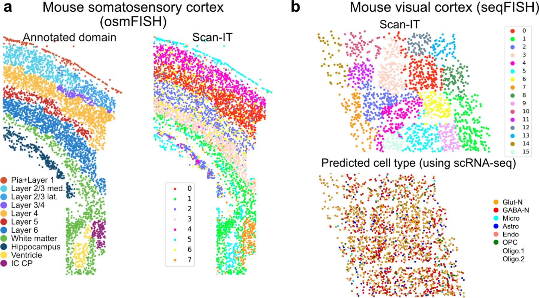
SCAN-IT segmentation of spatial imaging data. a. Mouse somatosensory cortex examined by osmFISH with annotated tissue domain from the original publication [2] and the domain segmentation by SCAN-IT. b. SCAN-IT domain segmentation based on mouse visual cortex datasets using seqFISH [21] and the cell types characterized using a paired single-cell RNA sequencing data in the original publication of the seqFISH data [21].

When applying SCAN-IT to a seqFISH data of mouse visual cortex with 1597 cells and 125 genes [21], we find 16 different spatial domains (Fig. 2b). Interestingly, the inferred tissue domains capture spatial regions of cells that exhibit collective information instead of different cell states or types. Specifically, each domain contains multiple different types of cells characterized by non-spatial clustering. This analysis suggests strong applicability of SCAN-IT and its validity.

3.2. Single-cell resolution spatial transcriptomics data

Next, we apply SCAN-IT to a single-cell resolution ST data of mouse somatosensory cortex obtained by seqFISH+ technique [5] with 523 cells and 10000 genes. The inferred tissue domains capture the spatial regions with two properties: a) within a given region cells of different annotation are well-mixed in space and b) different regions have different compositions of cells (Fig. 3a ). To further investigate the relations between the identified spatial domains and the cell types, we show the marker genes that are found to be differentially expressed in each inferred tissue domain (Fig. 3b,c). It is clear the top marker genes for the identified spatial domains are different from cell type marker genes. Together, this indicates that our segmentation identifies spatial domains with biological differences that are beyond the classical non-spatial cell clustering.

Figure 3:

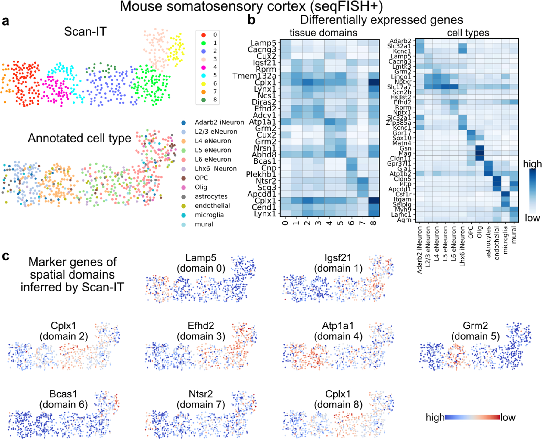
Inferred tissue domains of single-cell resolution ST data of mouse somatosensory cortex obtained using seqFISH+ technique. a. The SCAN-IT segmentation of the ST data and the manually annotated cell types of individual cells. b. The spatial marker genes of the tissue domains (left) and the marker genes of the annotated cell types (right). c. Spatial expression of the top spatial marker gene for each tissue domain.

3.3. Non-single-cell resolution spatial transcriptomics data

Due to current technological limitations, when increasing the tissue coverage or sequencing depth, the spatial resolution is often reduced, for example, leading to a loss of the individual cell resolution. We further evaluate SCAN-IT by analyzing datasets from two different techniques that measure gene expression at spatial spots with each spot containing a small number of cells rather than one cell.

The two datasets obtained by Visium technique on the coronal section and the sagittal posterior section of mouse brain contain 32285 genes, and 2702 and 3355 spatial spots, respectively [16]. The domain segmentation by SCAN-IT well captures the anatomical regions as revealed in the classical histological H&E stain images that have been well used as a tool for tissue segmentation (Fig. 4a,b).

Figure 4:

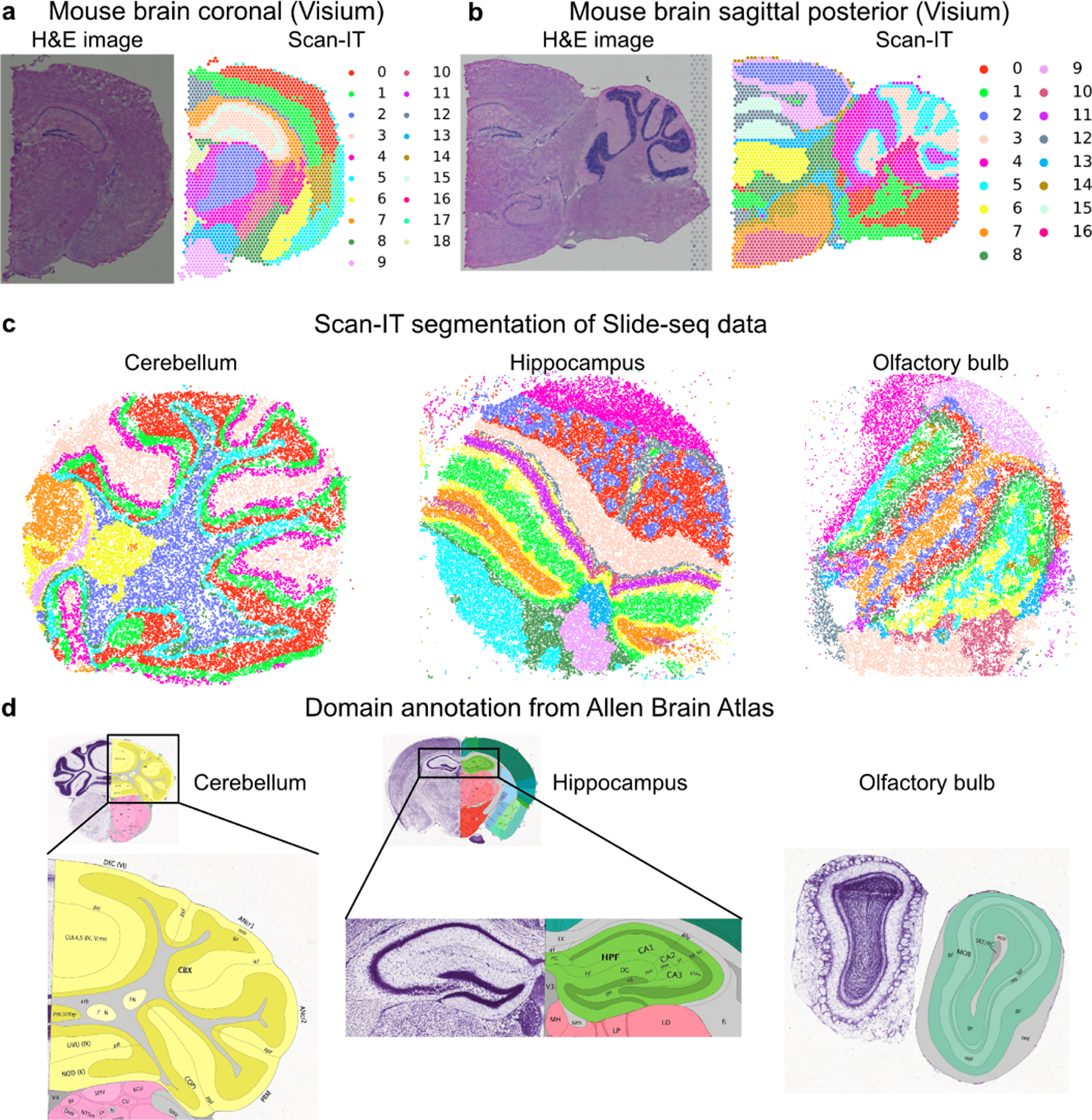
Segmentation of datasets with non-single-cell resolution. a. The H&E image and segmentation of Visium data of mouse brain coronal section. b. The H&E image and segmentation of Visium data of mouse brain sagittal posterior section. c. Segmentation of Slide-seq datasets of mouse cerebellum, hippocampus, and olfactory bulb. d. Ground-truth anatomical segmentation in the reference atlas from Allen Brain Atlas [9].

SCAN-IT also correctly detects tissue domains in three mouse spatial datasets from Slide-seq technique [14], namely, the cerebellum (24847 spots and 18906 genes), the hippocampus (38666 spots and 19869 genes), and the olfactory bulb (26316 spots and 18838 genes) compared to the ground-truth segmentation from Allen Brain Atlas [9] (Fig. 4c,d).

3.4. Comparison to other methods

Finally, we use a benchmark dataset with ground truth tissue domain segmentations [10] to compare our method with four recently developed methods, namely, spatialLIBD [10], smfishHmrf [3, 21], stLearn [13], and BayesSpace [20]. This benchmark contains twelve Visium datasets of human dorsolateral prefrontal cortex. The tissue domains were annotated manually in the original publication [10], which we use as the ground truth for benchmark. For the comparison, we use four standard metrics that measure the quality of a clustering given the ground-truth clustering including the normalized mutual information, adjusted Rand index, adjusted mutual information, and Fowlkes-Mallows index [11, 18] (Fig. 5).

Figure 5:

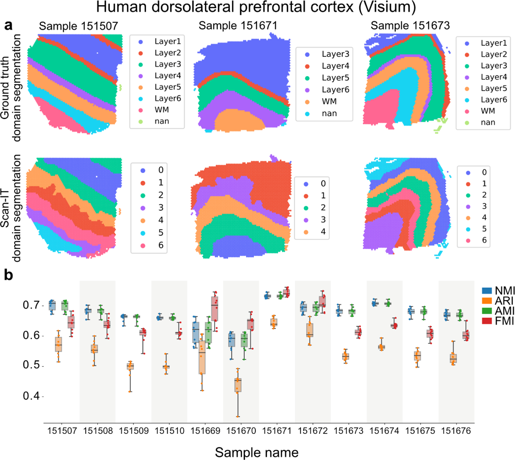
Benchmark of SCAN-IT on twelve Visium datasets with marker genes taken from the original publication [10]. For each sample, ten independent runs of SCAN-IT are carried out. a. The ground truth segmentation (determined by domain expert with prior knowledge) and the SCAN-IT segmentation with the median performance over the ten independent runs are shown for three representative samples for the three types of layouts. The ground truth labels the domain as layers 1 to 6 and white matter (WM) in the biological context, and in the unsupervised SCAN-IT domain segmentation, the domains are labeled with cluster numbers without biological interpretation. An accurate unsupervised domain segmentation should have a similar clustering of nodes compared to the ground truth. b. The performance of SCAN-IT in the ten independent runs over the twelve samples measured by normalized mutual information (NMI), adjusted Rand index (ARI), adjusted mutual information (AMI), and Fowlkes-Mallows index (FMI).

SCAN-IT with unbiased gene selection (top 3000 spatially variable genes identified by using SOMDE [6]) outperforms other methods regarding all four metrics while SCAN-IT with only the 126 manually picked spatial marker genes in the original study [10] further significantly improves the clustering performance (Table 1).

Table 1:

The performance (mean;median;standard deviation) of the methods measured by normalized mutual information (NMI), adjusted Rand index (ARI), adjusted mutual information (AMI), and Fowlkes-Mallows index (FMI) over the twelve benchmark datasets [10].

	NMI	ARI	AMI	FMI
spatialLIBD	0.430;0.416;0.053	0.288;0.283;0.056	0.429;0.414;0.053	0.459;0.473;0.034
smfishHmrf	0.479;0.513;0.070	0.334;0.354;0.061	0.478;0.512;0.070	0.480;0.483;0.061
stLearn	0.526;0.529;0.069	0.353;0.352;0.075	0.525;0.528;0.069	0.511;0.512;0.044
BayesSpace	0.598;0.622;0.083	0.447;0.488;0.108	0.597;0.621;0.083	0.574;0.572;0.068
SCAN-IT (SVgenes)	0.619;0.627;0.059	0.465;0.464;0.091	0.619;0.626;0.059	0.589;0.582;0.069
SCAN-IT (markers)	0.676;0.683;0.037	0.544;0.541;0.047	0.675;0.682;0.037	0.646;0.635;0.043

4. Conclusion

We have developed a method using graph neural networks approach to segment biological tissues, a major challenging task when analyzing the emerging spatial transcriptomics data. SCAN-IT has been evaluated on spatial transcriptomics datasets of various spatial resolutions for its applicability and accuracy, and found to outperform several existing methods on a benchmark dataset with ground-truth tissue domains. Formulating the tissue segmentation problem in spatial transcriptomics data as a graph/image segmentation problem establishes a new bridge between computer vision and spatial bioinformatics. In the experiments, we found that comparing to commonly used knn graphs, the alpha complex induced spatial neighborhood graph produces most accurate results and it can potentially improve performances of segmentation of broader point cloud data embedded in 2D or 3D. Finally, SCAN-IT is implemented as a user-friendly open-source Python package with extensive tutorials provided, and it is directly applicable to custom spatial transcriptomics data.

Figure 1:

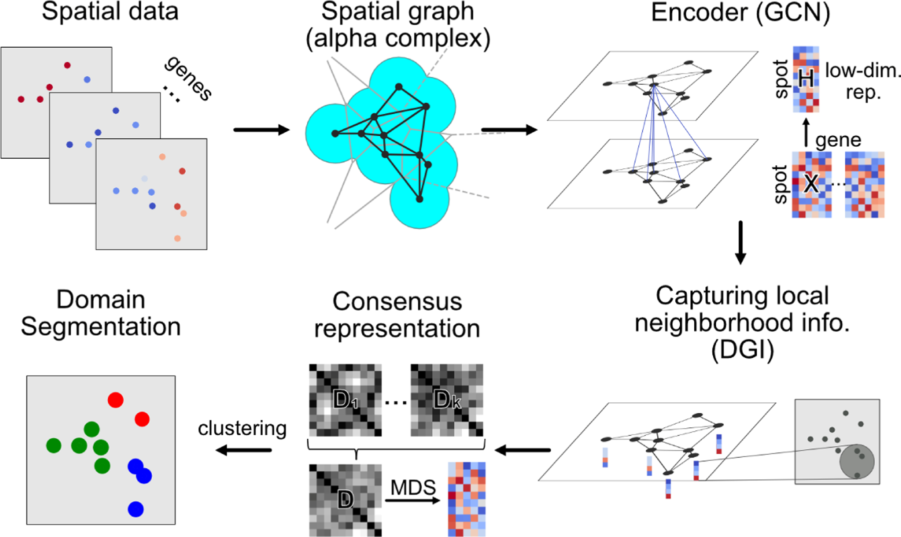
Overview of Scan-IT method. A spatial graph is constructed for the spatial spots of cells using alpha complex. A graph convolutional neural network is then used as an encoder trained using the deep graph infomax [17]. The tissue domains are segmented by performing clustering on a consensus low-dimensional representation obtained from multiple independently trained encoders or external embeddings.

References

- [1].Blondel Vincent D, Guillaume Jean-Loup, Lambiotte Renaud, and Lefebvre Etienne. Fast unfolding of communities in large networks. Journal of statistical mechanics: theory and experiment, 2008(10):P10008, 2008. [Google Scholar]
- [2].Codeluppi Simone, Borm Lars E, Zeisel Amit, Manno Gioele La, van Lunteren Josina A, Svensson Camilla I, and Linnarsson Sten. Spatial organization of the somatosen-sory cortex revealed by osmfish. Nature methods, 15(11):932–935, 2018. [DOI] [PubMed] [Google Scholar]
- [3].Dries Ruben, Zhu Qian, Dong Rui, Linus Eng Chee-Huat, Li Huipeng, Liu Kan, Fu Yuntian, Zhao Tianxiao, Sarkar Arpan, Bao Feng, et al. Giotto: a toolbox for integrative analysis and visualization of spatial expression data. Genome biology, 22(1):1–31, 2021. [DOI] [PMC free article] [PubMed] [Google Scholar]
- [4].Edelsbrunner Herbert and Mücke Ernst P. Three-dimensional alpha shapes. ACM Transactions on Graphics (TOG), 13(1):43–72, 1994. [Google Scholar]
- [5].Linus Eng Chee-Huat, Lawson Michael, Zhu Qian, Dries Ruben, Koulena Noushin, Takei Yodai, Yun Jina, Cronin Christopher, Karp Christoph, Yuan Guo-Cheng, et al. Transcriptome-scale super-resolved imaging in tissues by rna seqfish+. Nature, 568 (7751):235–239, 2019. [DOI] [PMC free article] [PubMed] [Google Scholar]
- [6].Hao Minsheng, Hua Kui, and Zhang Xuegong. SOMDE: a scalable method for identifying spatially variable genes with self-organizing map. Bioinformatics, 06 2021. btab471. [DOI] [PubMed] [Google Scholar]
- [7].Hjelm R Devon, Fedorov Alex, Lavoie-Marchildon Samuel, Grewal Karan, Bachman Phil, Trischler Adam, and Bengio Yoshua. Learning deep representations by mutual information estimation and maximization In International Conference on Learning Representations, 2019. [Google Scholar]
- [8].Kipf Thomas N. and Welling Max. Semi-supervised classification with graph convolutional networks In International Conference on Learning Representations (ICLR), 2017. [Google Scholar]
- [9].Lein Ed S, Hawrylycz Michael J, Ao Nancy, Ayres Mikael, Bensinger Amy, Bernard Amy, Boe Andrew F, Boguski Mark S, Brockway Kevin S, Byrnes Emi J, et al. Genome-wide atlas of gene expression in the adult mouse brain. Nature, 445(7124): 168–176, 2007. [DOI] [PubMed] [Google Scholar]
- [10].Maynard Kristen R, Collado-Torres Leonardo, Weber Lukas M, Uytingco Cedric, Barry Brianna K, Williams Stephen R, Catallini Joseph L, Tran Matthew N, Besich Zachary, Tippani Madhavi, et al. Transcriptome-scale spatial gene expression in the human dorsolateral prefrontal cortex. Nature neuroscience, 24(3):425–436, 2021. [DOI] [PMC free article] [PubMed] [Google Scholar]
- [11].Marina Meilӑ Comparing clusterings—an information based distance. Journal of multivariate analysis, 98(5):873–895, 2007. [Google Scholar]
- [12].Minaee Shervin, Boykov Yuri Y, Porikli Fatih, Plaza Antonio J, Kehtarnavaz Nasser, and Terzopoulos Demetri. Image segmentation using deep learning: A survey. IEEE Transactions on Pattern Analysis and Machine Intelligence, 2021. [DOI] [PubMed]
- [13].Pham Duy Truong, Tan Xiao, Xu Jun, Grice Laura F, Lam Pui Yeng, Raghubar Arti, Vukovic Jana, Ruitenberg Marc J, and Nguyen Quan Hoang. stlearn: integrating spatial location, tissue morphology and gene expression to find cell types, cell-cell interactions and spatial trajectories within undissociated tissues. bioRxiv, 2020.
- [14].Rodriques Samuel G, Stickels Robert R, Goeva Aleksandrina, Martin Carly A, Murray Evan, Vanderburg Charles R, Welch Joshua, Chen Linlin M, Chen Fei, and Macosko Evan Z. Slide-seq: A scalable technology for measuring genome-wide expression at high spatial resolution. Science, 363(6434):1463–1467, 2019. [DOI] [PMC free article] [PubMed] [Google Scholar]
- [15].Shi Yilei, Li Qingyu, and Zhu Xiao Xiang. Building segmentation through a gated graph convolutional neural network with deep structured feature embedding. ISPRS Journal of Photogrammetry and Remote Sensing, 159:184–197, 2020. [DOI] [PMC free article] [PubMed] [Google Scholar]
- [16].Ståhl Patrik L, Salmén Fredrik, Vickovic Sanja, Lundmark Anna, Navarro José Fernández, Magnusson Jens, Giacomello Stefania, Asp Michaela, Westholm Jakub O, Huss Mikael, et al. Visualization and analysis of gene expression in tissue sections by spatial transcriptomics. Science, 353(6294):78–82, 2016. [DOI] [PubMed] [Google Scholar]
- [17].Veličković Petar, Fedus William, Hamilton William L., Liò Pietro, Bengio Yoshua, and Hjelm R Devon. Deep graph infomax In International Conference on Learning Representations, 2019. [Google Scholar]
- [18].Vinh Nguyen Xuan, Epps Julien, and Bailey James. Information theoretic measures for clusterings comparison: Variants, properties, normalization and correction for chance. The Journal of Machine Learning Research, 11:2837–2854, 2010. [Google Scholar]
- [19].Viswanath Satish and Madabhushi Anant. Consensus embedding: theory, algorithms and application to segmentation and classification of biomedical data. BMC bioinformatics, 13(1):1–20, 2012. [DOI] [PMC free article] [PubMed] [Google Scholar]
- [20].Zhao Edward, Stone Matthew R, Ren Xing, Guenthoer Jamie, Smythe Kimberly S, Pulliam Thomas, Williams Stephen R, Uytingco Cedric R, Taylor Sarah EB, Nghiem Paul, Bielas Jason H, and Gottardo Raphael. Spatial transcriptomics at subspot resolution with bayesspace. Nature Biotechnology, pages 1–10, 2021. [DOI] [PMC free article] [PubMed]
- [21].Zhu Qian, Shah Sheel, Dries Ruben, Cai Long, and Yuan Guo-Cheng. Identification of spatially associated subpopulations by combining scrnaseq and sequential fluorescence in situ hybridization data. Nature biotechnology, 36(12):1183–1190, 2018. [DOI] [PMC free article] [PubMed] [Google Scholar]