

Abstract
Purpose
To develop and evaluate a parallel imaging and convolutional neural network combined image reconstruction framework for low‐latency and high‐quality accelerated real‐time MR imaging.
Methods
Conventional Parallel Imaging reconstruction resolved as gradient descent steps was compacted as network layers and interleaved with convolutional layers in a general convolutional neural network. All parameters of the network were determined during the offline training process, and applied to unseen data once learned. The proposed network was first evaluated for real‐time cardiac imaging at 1.5 T and real‐time abdominal imaging at 0.35 T, using threefold to fivefold retrospective undersampling for cardiac imaging and threefold retrospective undersampling for abdominal imaging. Then, prospective undersampling with fourfold acceleration was performed on cardiac imaging to compare the proposed method with standard clinically available GRAPPA method and the state‐of‐the‐art L1‐ESPIRiT method.
Results
Both retrospective and prospective evaluations confirmed that the proposed network was able to images with a lower noise level and reduced aliasing artifacts in comparison with the single‐coil based and L1‐ESPIRiT reconstructions for cardiac imaging at 1.5 T, and the GRAPPA and L1‐ESPIRiT reconstructions for abdominal imaging at 0.35 T. Using the proposed method, each frame can be reconstructed in less than 100 ms, suggesting its clinical compatibility.
Conclusion
The proposed Parallel Imaging and convolutional neural network combined reconstruction framework is a promising technique that allows low‐latency and high‐quality real‐time MR imaging.
Keywords: compressed sensing, convolutional neural network, deep learning, low‐latency, parallel imaging, real‐time magnetic resonance imaging
1. Introduction
With tremendous advances in MRI hardware performance and fast imaging techniques in the past two decades, real‐time MRI has shown great potentials for a number of challenging applications, such as speech imaging,1, 2 cardiac imaging,3, 4, 5 functional imaging,6, 7 and interventional MRI.8, 9 To achieve sufficient frame rate, real‐time MRI typically requires significant k‐space undersampling to accelerate the data acquisition. As a result, advanced image reconstruction algorithms are needed to remove aliasing artifacts arising from k‐space undersampling. Two broad categories of these techniques are parallel imaging and compressed sensing.10, 11, 12 Parallel imaging takes advantage of the signal correlations between different coil elements of a receiver coil array to estimate the missing k‐space data or calculate the aliasing free image by inverting the sensitivity encoding process of MRI.10, 11 Compressed sensing algorithms use the image sparsity under certain mathematical transformations to reduce the size of solution space and use a nonlinear process to recover the image from the reduced solution space.12, 13, 14 For those real‐time MRI applications that require user interaction or real‐time decision making based on image feedback,15, 16 such as interventional MRI, there are a number of requirements that may be different from conventional diagnostic MRI applications. In addition to generic performance metrics such as spatial and temporal resolution, these real‐time MRI applications often have more stringent requirements with regard to geometric distortion of the images and image reconstruction latency, which is the time interval between the end of data acquisition and the completion of image reconstruction. For applications that only require fast data acquisition,17, 18 slower reconstruction methods may be used. For example, Uecker et al.19 demonstrated 1.5 mm2 and 20 ms spatial/temporal resolution real‐time MRI with a 2.5 s per frame reconstruction time. In another real‐time MRI study by Lingala et al.20, the authors used a through time spiral GRAPPA method21 for real‐time speech imaging with a reconstruction latency per frame of 114 ms and a modest spatial resolution of 2.4 mm2. More recently, several more reconstruction approaches, such as Borisch et al.22 using cluster computing, Sorensen et al.23 using non‐Cartesian trajectory and GPU computation, and Majumdar et al.24 using compressed sensing and dedicated fast computation libraries, were proposed for high spatial and temporal resolution real‐time imaging.
Despite the promise of non‐Cartesian trajectories and CS‐based iterative approaches in real‐time imaging, these methods are limited in certain aspects: (a). Non‐Cartesian trajectories are sensitive to different kinds of system imperfections, such as gradient delays and field inhomogeneities, which could lead to image blurring and geometric distortions in real‐time MRI. Therefore, these non‐Cartesian approaches usually require extra pre/postprocessing time for reconstruction.25 (b). For CS applications, fixed sparsifying transforms are typically used in most CS‐based algorithms. Although there exist various simple yet powerful sparsifying transforms, such as wavelet,12 total variation,14 that could be useful for many applications, they may be too simple to capture the underlying complex image features for all imaging applications26; (c) Solvers for iterative algorithm need to be specially designed or modified so that low‐latency online reconstruction is feasible.14 Recent developments in deep learning‐based MRI image reconstruction may provide solutions to these issues. Taking the experiences from early success in image classification27 and recent improvement in image restoration28 and super‐resolution,29 several neural network architectures have been proposed30, 31, 32, 33, 34 to learn the (nonlinear) mapping from artifact‐contaminated images due to k‐space undersampling to the fully sampled reference images. This could greatly relax the need for using non‐Cartesian k‐space trajectories to achieve incoherent sampling, and alleviate the need for optimizing the sparsifying transform. Automated transform by manifold approximation (AUTOMAP)35 as a general framework for image reconstruction consisting of fully connected layers followed by a convolutional autoencoder, directly maps the k‐space data to the image domain. A stack of autoencoders has also been also proposed36 to map undersampled radial images to high‐quality fully sampled images. Deep residual networks followed by linear fully connected layers have been used37 to reconstruct the image from compressively sensed measurements. Deep neural networks have also been used to explore much more effective image priors and sparsifying transforms from a given dataset and combined with conventional CS methods. As proposed in Ref. [38], the ADMM algorithm is used to solve the inverse problems such as CS‐MRI. Another interesting technique34 was recently reported using a variational autoencoder for learning the effective priors to reconstruct knee datasets. Generative adversarial networks (GANs) have been proposed to achieve a higher perceptual quality in inverse problems such as super resolution.39, 40, 41, 42 Additional new techniques have been proposed to increase the sharpness and preserve the texture information in MR reconstruction tasks.43, 44 Transfer learning has also been explored as an effective image reconstruction method.45, 46
In this work, we sought to develop a Parallel Imaging and Convolutional Neural Network (PI‐CNN) combined reconstruction framework and apply it to two‐dimensional (2D) real‐time imaging for low‐latency online reconstruction. Compared with most existing neural network‐based methods30, 31, 32, 33 that only learn the mapping from single‐coil data, our framework integrated multicoil k‐space data and utilize them through parallel imaging. We demonstrate the capability of our framework on two different applications: real‐time cardiac imaging at 1.5 T and real‐time abdominal imaging at 0.35 T. Retrospective studies were performed to compare the proposed method against an existing single‐coil–based neural network reconstruction32 and a PI‐CS method.47 Prospective examples were also shown to demonstrate the improved temporal resolution from the accelerated acquisition and our image PI‐CNN reconstruction algorithm.
2. Materials and method
2.A. Problem formulation
To reconstruct undersampled data in an accelerated MR acquisition, an ill‐posed linear inverse problem can be formulated as follows:
| (1) |
where is the target image to be reconstructed; is the acquired multicoil undersampled k‐space data padded with zeros at unsampled k‐space locations; is a chain of linear operators including point‐wise multiplication of sensitivity maps, forward Fourier transform, and point‐wise multiplication of undersampling mask; and is measurement noise. Since the system of Eq. (1) is ill‐posed, as well as the fact that measured data are noisy in practical scenarios, minimizing the least square error of Eq. (1) with additional regularization term is usually used to prevent overfitting to noisy image, given by the following optimization problem:
| (2) |
where is the regularization parameter that trades off the data fidelity term and regularization term.
Common choices of are norm, which is the sum of absolute values of every element in a vector or matrix, wavelets and total variation, aiming at exploiting the sparsity of the underlying image in the transform domain. However, predetermined sparsifying transforms only preserve certain features of the image and lack the generality of representing complex natural features. For example, total variation increases at edges of the image and therefore favors piece‐wise constant structures. As a result, image reconstructions using total variation as regularizations could result in oversmoothed images with blurred boundaries between structures. Inspired by early work of using sparse dictionary learning‐based regularization for MR reconstruction,26 and more recent work of using convolutional neural networks (CNN) for natural image reconstruction,48 we propose to use a general CNN‐based regularization in this work. Specifically, assume maps an artifact‐contaminated image, mainly caused by k‐space undersampling and results in structural ghosting aliasing or incoherent noise‐like artifacts on image, to an artifact‐free image. It can be represented by multiple layers of convolutional kernels parameterized by .48, 49 Hence, a compact representation of this mapping is:
| (3) |
Incorporating Eq. (3) as a regularization term into Eq. (2) gives us the following reconstruction problem:
| (4) |
where is the image derived from undersampled zero‐filled k‐space data. In case the mapping is already learned with known parameters , equation [4] can be solved using the gradient descent algorithm with some initial image :
| (5) |
where is reconstructed image at iteration , is the step size at iteration , and is the adjoint chain of linear operators. Although the global minimal of Eq. (4), which is a pure quadratic optimization problem, can be obtained by setting its derivative to be zero, and solving a system of linear equations through direct matrix inversion or pseudo‐inversion, we chose to solve it with the gradient descent algorithm due to the large size of the coefficient matrix () when multiple coil sensitivity maps are included, as well as its poor conditioning when undersampling factor is high. For previously mentioned natural image reconstruction task,48, 49 learning parameters for is usually performed in image domain only. However, by incorporating the k‐space data in training, which is a representation of the image in the spatial‐frequency domain, we hypothesize that we will be able to improve image reconstructions compared to traditional image‐based training in terms of image artifact removal when the image was acquired with k‐space undersampling. In several previously proposed CNN‐based MR reconstruction methods32, 33 that utilized k‐space data for reconstruction, the investigators either utilized the k‐space data after the network training is completed33 or only considered single‐coil data.32 On the contrary, the proposed approach alternatively learns parameters through CNN and solves the parallel imaging problem in equation [5], using a cascaded network architecture32 as shown in Fig. 1. Our approach not only generalizes the common regularization terms used in CS methods but also allows the CNN to better use the acquired multicoil k‐space data by incorporating parallel imaging.
Figure 1.
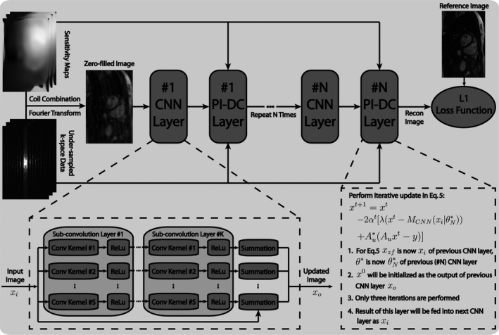
Structure of the proposed parallel imaging and convolutional neural network (PI‐CNN) combined reconstruction network. The PI‐CNN network consists of composite CNN layers and PI‐DC layers cascaded in series. Each composite CNN layer contains subconvolution layers.
2.B. Network design
As illustrated in Fig. 1, our network consists of composite CNN layers and Parallel Imaging data consistency (PI‐DC) layers cascaded in series. Each subconvolution layer in the CNN layer has filters with size 3 × 3. Complex images are input to CNN layers in two separate channels (real and imaginary), which are combined back to a single‐channeled complex image at the output of CNN layers. In the PI‐DC layer, the output of the preceding CNN layer is iteratively updated according to Eq. (5). In consideration of computation time, three iterations are performed in the PI‐DC layer with set to 0.4 empirically in Eq. (5).
During the offline network training process, the goal is to find an optimal parameter set for the convolution filters. Since there is no updatable parameter in the PI‐DC layer, a total of parameters need to be trained. To set up this procedure, we minimize a loss function over a set of paired reconstructed image and reference image with respect to . Based on previous literature,50, 51 we choose L1 norm instead of conventional L2 norm as our main loss function, which is defined as follows:
| (6) |
where and is the ith pair of images in the set of size , and is the operation that takes the magnitude of the complex image. To prevent model overfitting, we further added an L2 regularization on the network parameters. Due to the fact that is not differentiable at the origin point, we relaxed it with in our practical implementation. The above optimization problem is solved by the well‐known back‐propagation algorithm,52 that is, applying the chain rule for parameters of the layer:
| (7) |
where is the output of (m+1)th layer from a total of layers including the subconvolution layers and PI‐DC layers. Note that we are performing an end‐to‐end training, and therefore, the back‐propagation starts from the last cascaded layer. Although no parameter is updated in the PI‐DC layer, the derivative of its output with respect to its input still needs to be calculated, so that the gradient can flow backward. In other words, the derivative of layer output in both CNN and PI‐DC layers, with respective to the corresponding layer input, needs to be evaluated so that every term on the righthand side of Eq. (7) is well‐defined. For each PI‐DC layer, which consists of three gradient descent update steps shown in Eq. (5), it can be unpacked as three separate sublayers, with the input as , and output as . This can simplify the calculation of derivative for one PI‐DC layer to be a chain of three derivatives associated with each of these thee sublayers, calculated as . For the resting CNN layers, the derivatives used in the back‐propagation is calculated using numerical differentiation provided in the backend network libraries mentioned at the end of section “Network Training.”
For comparison purposes, the single‐coil–based network described in Ref. [18] was also implemented in this work. In this network, the k‐space data in equation [4] is replaced with a synthesized single‐coil k‐space data, which is generated by inverse Fourier transform of fully sampled multicoil k‐space data to image domain, coil combination in image domain using SENSE,10 another Fourier transform, and retrospective k‐space undersampling. The chain operator only involves performing Fourier transform and applying the undersampling mask. Moreover, Eq. (5) is replaced with a single‐step k‐space data substitution operation. Equation (6) in Ref. [32] describes this operation in more details.
2.C. Data acquisition
To evaluate the performance of the proposed PI‐CNN method and demonstrate its utility, we tested our strategy for real‐time cardiac and abdominal imaging applications. The study was approved by our institutional review board, and each subject provided written informed consent. For cardiac imaging, 20 healthy volunteers were scanned on a 1.5 T MRI scanner (Avanto Fit, Siemens Medical Solutions, Erlangen, Germany) using a standard bSSFP sequence with a 32‐channel body coil array (TE/TR = 1.5/3 ms, flip angle = 60°, bandwidth = 814 Hz/pixel, field of view = 260 − 350 × 160 – 220 mm2, matrix size = 192 × 122, slice thickness = 6 mm2). In each volunteer, 250 short‐axis view fully sampled images (temporal resolution = 3 frames per second) at various slice locations across the heart were acquired during free‐breathing without ECG gating. The image acquisition time was 84 s for each volunteer. Prospectively 4X undersampled data using a one‐dimensional (1D) variable density Poisson‐disc pattern12 were acquired in two additional volunteers in the short‐axis view. As a comparison, a separate cardiac cine MRI using conventional 3X GRAPPA acceleration with 20 reference lines and partial Fourier 5/8, corresponding to a 4X net acceleration, was acquired at the same slice locations as our Poisson‐disc undersampled data. For both undersampled acquisitions, imaging time was 21 s.
For abdominal imaging, a total of eight healthy volunteers and eight liver cancer patients were scanned on a 0.35 T MRI‐guided radiotherapy (MRgRT) system (MRIdian, ViewRay, Cleveland, OH) using a standard bSSFP sequence with a 12‐channel body coil array (TE/TR = 1.7/3.4 ms, flip angle = 110°, bandwidth = 548 Hz/pixel, field of view = 300 – 420 × 180 – 250 mm2, matrix size = 192 × 114, slice thickness = 8 mm2). The MRgRT system is capable of simultaneous MRI and radiotherapy, but was only used as an MRI scanner in the study. In each volunteer and patient, 250 sagittal fully sampled images (temporal resolution = 3 fps) at various locations of the liver region (covering the tumor for patients) were acquired during free breathing. The image acquisition time was 84 s.
2.D. Network training
Both the proposed network and the single‐coil–based network described in Ref. [18] were trained using retrospectively undersampled data paired with their corresponding fully sampled reference data. As mentioned above, SENSE reconstruction10 was used to generate single‐coil images from multicoil images in the single‐coil–based network.32 In the proposed network, SENSE type reconstruction was used in the PI‐DC layer to enforce data consistency under the parallel imaging framework. For cardiac imaging, 3750 short‐axis image pairs from 15 volunteers were used for training. For abdominal imaging, 3000 sagittal image pairs from 6 volunteers and 6 patients were used. The network trainings were performed separately for cardiac imaging datasets and abdominal imaging datasets. For a given undersampling factor (3X‐5X), the Poisson‐disc undersampling masks were varied for the training datasets so that the network learns various aliasing patterns. The coil sensitivity maps used in the proposed method were calibrated from the 24 × 24 central k‐space region using ESPIRiT.47
Both networks were implemented in Python using Theano and Lasagne libraries. Parameters of the networks were initialized with He initialization,53 trained with Adam optimizer54 using following parameters: , , and . One thousand epochs with minibatch size of 16 were used. All training and experiments were performed on a Linux PC (8 Core/4 GHz, 64 GB, Nvidia GTX 760). It took approximately 1 day to train each network.
2.E. Evaluation
The proposed PI‐CNN network was tested on data from the remaining five volunteers in cardiac imaging, and the remaining two volunteers and two patients in abdominal imaging. All test data were not included in the training process.
In the first step, we evaluated the effect of different and in the proposed PI‐CNN network. Two experiments were performed: (a) We fixed for each composite CNN layer but varied . This experiment would show the value of increasing cascade iteration. (b). We compared two architectures, both with a total number of 25 layers: and . The first architecture benefits from the repeated enforcement of data consistency while the second one can extract very deep features.55 This experiment allowed us to evaluate the benefit of using k‐space data within a network. For each network trained in the two experiments, a fourfold acceleration factor was set.
Next, we evaluated the performance of the proposed network against a single‐coil–based network32 and L1‐ESPIRiT,47 a state‐of‐the‐art PI‐CS reconstruction method, through a retrospective study on the cardiac imaging. Based on experiments in the first step, we set for both the proposed network and the single‐coil–based network. Threefold to fivefold acceleration factors were evaluated with the 1D variable density Poisson‐disc undersampling pattern. L1‐ESPIRiT was performed using a previously described tool (Berkeley Advanced Reconstruction Toolbox, BART),56 with the same sensitivity maps used for network reconstruction. All hyperparameters for L1‐ESPIRiT such as the number of iterations and regularization parameters were tuned empirically to provide best image quality based on visual assessment.
Since our network learns to de‐alias undersampled artifact‐contaminated images in general, it is possible that the network trained at one acceleration factor may be used to reconstruct images acquired with a different acceleration factor. To explore this, we used the network trained with the intermediate fourfold acceleration factor in the previous experiment to reconstruct images retrospectively undersampled with threefold to fivefold acceleration factors. As a comparison, these images were also reconstructed using the networks trained with the corresponding acceleration factors. L1‐ESPIRiT, as a representative of nontraining‐based methods, was also performed.
As a next step, we further evaluated the performance of the proposed PI‐CNN network on the prospectively undersampled data. However, it is not possible to reconstruct them with the single‐coil–based network.32 This is because it only works with the synthesized single‐coil data (i.e., it is trained on the synthesized coil‐combined image and coil‐combined retrospectively undersampled k‐space data), while the acquired prospective undersampled k‐space data have multiple channels and there is no easy way to derive coil‐combined undersampled k‐space data from that. Therefore, we only compare it with the L1‐ESPIRiT reconstruction based on the same data, as well as the additionally acquired GRAPPA accelerated data.
Next, to evaluate the proposed network in a different body site, a different SNR scenario, and to demonstrate its potential in clinical utility in patients, we performed a study for abdominal imaging acquired at 0.35 T. The patients in this evaluation were liver cancer patients who underwent MR‐guided radiation therapy using our MRgRT system. The abdominal images were acquired immediately after the patient finished a treatment session. The k‐space data from one volunteer and two patients were retrospectively undersampled by a threefold acceleration factor, and reconstructed with the proposed network and L1‐ESPIRiT. Because of the improved performance of the proposed network over single‐coil–based network based on cardiac imaging (shown in the Section 3), here we used the clinically available linear PI reconstruction GRAPPA as the alternative comparison, based on the same data that were retrospectively undersampled with a regular pattern and net acceleration factor of threefold.
Finally, we assessed the robustness of the proposed network by performing a fourfold cross‐validation study. Specifically, we evenly divided the datasets acquired from cardiac and abdominal imaging experiments into four subsets, with a subset size of 1250 images for cardiac imaging, and 1000 images for abdominal imaging. The retrospective reconstruction evaluation process, as detailed above, was then repeated four times for each imaging experiment, such that each time, one of four subsets was used as a testing dataset and the other thre subsets were combined together to form the training dataset. Corresponding comparisons with other algorithms (single‐coil–based network and L1‐ESPIRiT for cardiac imaging, GRAPPA and L1‐ESPIRiT for abdominal imaging) were also performed on the testing dataset.
2.F. Data analysis
To compare the different reconstruction strategies quantitatively in the cross‐validation evaluation, both normalized root mean square errors (nRMSE) and structural similarity index (SSIM)56 were calculated between each frame of the reference images and images reconstructed with the different strategies (proposed network, single‐coil based network, L1‐ESPIRiT and GRAPPA). The calculated nRMSE and SSIM were averaged across all frames and all volunteers/patients. Although reduction in nRMSE indicates greater fidelity to the original image, an SSIM value of 1 indicates a perfectly identical pair and the SSIM value decreases as the images differ. Quantitative measurements were reported separately for each cross‐validation repetition. In addition to the quantitative evaluation, the image quality of all reconstructed images, using a single‐coil–based network, the proposed network, and L1‐ESPIRiT, from five testing volunteers in the cardiac imaging were subjectively evaluated by two readers with an experienced knowledge of MR cardiology and were blinded to the MRI reconstruction methods. The presented images were graded using a 4‐point ordinal scale in terms of image sharpness (1: no blurring, 2: mild blurring, 3: moderate blurring, 4: severe blurring), and overall image quality (1: excellent, 2: good, 3: fair, 4: poor). Reported subjective scores were averaged over the two readers.
3. Results
Figure 2 shows example images reconstructed from the six networks that have different cascading depths (). As increased, the reconstructed images had fewer aliasing artifacts (red arrows), sharper tissue boundary (yellow arrows) and better delineated myocardium (green arrows). The rate of improvement and artifact reduction slowed down as increased. There was obvious difference between the () image and the () image. The difference between the () image and the () image was subtler, although the () image required increased reconstruction time (46 ms for and 90 ms for to reconstruct a 12‐channel data) and potentially increased sensitivity to overfitting. Therefore, we used the network for the remaining study of this work.
Figure 2.
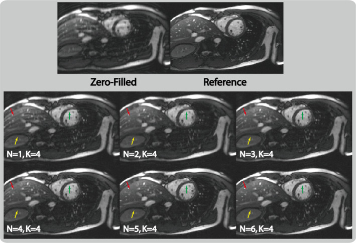
Example images reconstructed with the proposed parallel imaging and convolutional neural network (PI‐CNN) network using different network depths (i.e., number of composite CNN and parallel imaging data consistency layers) at fourfold acceleration factor. With increased depth ( from 1 to 6), the reconstructed image has less aliasing artifact (red arrows) and sharper edges (yellow and green arrows), although this comes with longer reconstruction time. The network with represents a good balance between image quality and required reconstruction time. [Color figure can be viewed at wileyonlinelibrary.com]
Figure 3 shows the comparison of the two network architectures that have the same total number of 25 layers on selected reconstructed frames. As illustrated, the architecture that employs very deep convolution layers () for feature extraction was not able to remove residual aliasing artifacts (blue arrows) and failed to recover sharp myocardium boundaries (red arrows). On the contrary, using the same size of training data, the interleaved architecture () reconstructed much cleaner and sharper images, benefitting from the fact that it consistently provides an updated improved image from a PI reconstruction for each composite CNN layer.
Figure 3.
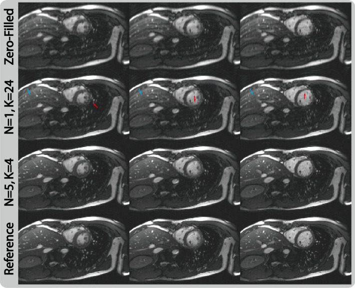
Selected reconstructed images of retrospective fourfold acceleration at three cardiac phases from two networks that have the same number of total layers but different architectures. For the network that has very deep convolution layers (), it fails to remove residual aliasing artifacts and sharpen the edges. On the other hand, the proposed cascaded architecture () allows good utilization of the feature extraction from convolutional neural network layers and data consistency enforcement from PI‐DC layers, and produces cleaner and sharper reconstructions. [Color figure can be viewed at wileyonlinelibrary.com]
To better understand how the proposed network utilizes the interleaving CNN and PI‐DC structure, Fig. 4 shows the intermediate images from each of the composite CNN layers (top row) and PI‐DC layers (bottom row) within the proposed network. Since end‐to‐end training was used, the intermediate layers internally learned to correct for the errors caused by the previous layers, and thus produced from the final layer images that were similar to the reference image.
Figure 4.
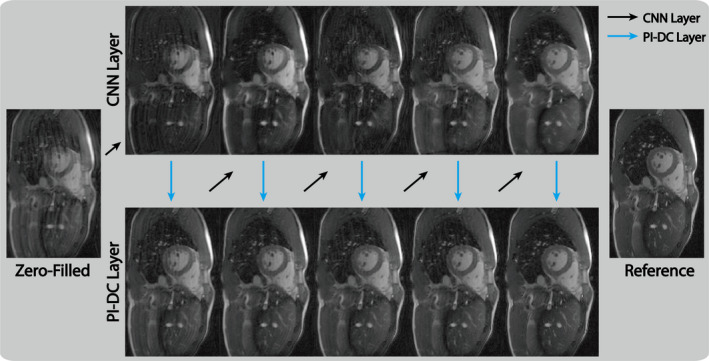
Intermediate network layer outputs of the parallel imaging and convolutional neural network for a retrospectively fourfold undersampled data. We observe overall continuously suppression of aliasing artifacts and sharpening of fine structures as the data pass through each cascaded layer. Due to the end‐to‐end training, our proposed parallel imaging data consistency network can internally correct for these deviations and produce an artifact‐free image after the final layer. [Color figure can be viewed at wileyonlinelibrary.com]
Figure 5 shows representative images reconstructed from zero‐filling, single‐coil–based network,32 proposed network, L1‐ESPIRiT, and fully sampled reference data. With threefold undersampling, all three strategies were able to reconstruct images with acceptable quality. With fourfold undersampling, single‐coil–based network reconstructed an image with apparent residual aliasing artifact (white arrow) and oversmoothed blocky artifacts (yellow arrow). L1‐ESPIRiT similarly had blurred myocardium (red arrow) and small blood vessel (blue arrow). The proposed network, however, could reconstruct similar image compared with the reference. At fivefold acceleration, the proposed PI‐CNN method started to show oversmoothed images (green arrows). The other two methods had similar reconstruction errors with fourfold undersampling. These observations correlate well with the numerical analysis shown in Table I and the subjective scores shown in Table II.
Figure 5.
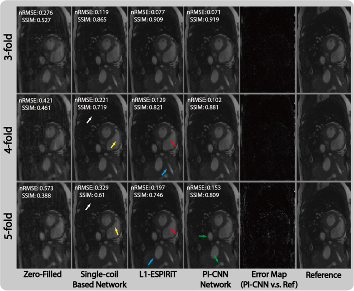
Comparison of different reconstruction strategies at three acceleration factors for short‐axis cardiac acquisition. From left to right, each column represents selected cardiac frame reconstructed with zero‐filling, single‐coil–based network, L1‐ESPIRiT, proposed parallel imaging and convolutional neural network (PI‐CNN) and reference, respectively. Normalized residual error maps between the PI‐CCN reconstructions and the reference are shown to demonstrate the magnitude of errors. As expected, as the acceleration rate increases, there is more residual errors. [Color figure can be viewed at wileyonlinelibrary.com]
Table I.
Quantitative comparisons of the different reconstruction strategies and the different undersampling factors in the cardiac and abdominal imaging applications with regard to nRMSE and SSIM.
| Experiments | Recon. methods | nRMSE | SSIM |
|---|---|---|---|
| Cardiac 3‐fold | Zero‐filling | 0.27 ± 0.04 (min:0.25, max:0.31)* | 0.53 ± 0.02 (min:0.49, max:0.56)* |
| Single‐coil Network | 0.11 ± 0.03 (min:0.1, max:0.13)* | 0.86 ± 0.02 (min:0.83, max:0.9) | |
| L1‐ESPIRiT | 0.07 ± 0.04 (min:0.06, max:0.09) | 0.91 ± 0.01 (min:0.88, max:0.92) | |
| PI‐CNN Network | 0.07 ± 0.03 (min:0.06, max:0.09) | 0.91 ± 0.03 (min:0.87, max:0.92) | |
| Cardiac 4‐fold | Zero‐filling | 0.42 ± 0.01 (min:0.37, max:0.46)* | 0.46 ± 0.02 (min:0.42, max:0.48)* |
| Single‐coil Network | 0.21 ± 0.02 (min:0.18, max:0.24)* | 0.73 ± 0.04 (min:0.68, max:0.78)* | |
| L1‐ESPIRiT | 0.12 ± 0.03 (min:0.1, max:0.15) | 0.82 ± 0.01 (min:0.8, max:0.84) | |
| PI‐CNN Network | 0.09 ± 0.03 (min:0.08, max:0.13) | 0.88 ± 0.02 (min:0.86, max:0.89) | |
| Cardiac 5‐fold | Zero‐filling | 0.57 ± 0.03 (min:0.52, max:0.59)* | 0.38 ± 0.04 (min:0.35, max:0.43)* |
| Single‐coil Network | 0.31 ± 0.02 (min:0.28, max:0.33)* | 0.62 ± 0.01 (min:0.6, max:0.64)* | |
| L1‐ESPIRiT | 0.19 ± 0.01 (min:0.18, max:0.21) | 0.75 ± 0.02 (min:0.74, max:0.77) | |
| PI‐CNN Network | 0.14 ± 0.04 (min:0.11, max:0.16) | 0.81 ± 0.02 (min:0.79, max:0.82) | |
| Abdominal 3‐fold | Zero‐filling | 0.29 ± 0.02 (min:0.25, max:0.31)* | 0.51 ± 0.01 (min:0.5, max:0.53)* |
| Single‐coil Network | 0.15 ± 0.02 (min:0.14, max:0.17)* | 0.81 ± 0.02 (min:0.79, max:0.83)* | |
| L1‐ESPIRiT | 0.10 ± 0.01 (min:0.09, max:0.12) | 0.85 ± 0.04 (min:0.82, max:0.89) | |
| PI‐CNN Network | 0.08 ± 0.02 (min:0.07, max:0.1) | 0.90 ± 0.02 (min: 0.88, max:0.91) |
nRMSE: normalized root mean square error; SSIM: structural similarity index.
Statistically significant difference between the labeled reconstruction method and the proposed parallel imaging and convolutional neural network (PI‐CNN) method.
Table II.
Subjective image quality scores in terms of image sharpness and overall image quality evaluated on the different reconstruction strategies and the different undersampling factors for cardiac imaging.
| Experiments | Recon. method | Image sharpness | Overall quality |
|---|---|---|---|
| Cardiac 3‐fold | Single‐coil Network | 1.65 ± 0.16 (min:1, max:3) | 1.32 ± 0.06 (min:1, max:3) |
| PI‐CNN Network | 1.54 ± 0.18 (min:1, max:2) | 1.26 ± 0.12 (min:1, max:2) | |
| L1‐ESPIRiT | 1.36 ± 0.22 (min:1, max:2) | 1.21 ± 0.18 (min:1, max:2) | |
| Cardiac 4‐fold | Single‐coil Network | 2.84 ± 0.12 (min:1, max:4)* | 2.55 ± 0.32 (min:1, max:4)* |
| PI‐CNN Network | 2.05 ± 0.07 (min:1, max:3) | 1.98 ± 0.19 (min:1, max:3) | |
| L1‐ESPIRiT | 2.18 ± 0.11 (min:1, max:3) | 2.08 ± 0.34 (min:1, max:3) | |
| Cardiac 5‐fold | Single‐coil Network | 3.52 ± 0.43 (min:2, max:4)* | 3.32 ± 0.38 (min:2, max:4)* |
| PI‐CNN Network | 3.04 ± 0.35 (min:2, max:4) | 2.86 ± 0.26 (min:2, max:4) | |
| L1‐ESPIRiT | 3.11 ± 0.26 (min:2, max:4) | 2.92 ± 0.42 (min:2, max:4) |
Statistically significant difference between the labeled reconstruction method and the proposed parallel imaging and convolutional neural network (PI‐CNN) method.
Figure 6 shows the results of applying the proposed network trained with one acceleration factor to reconstruct images undersampled with other acceleration factors. Applying the network trained on fourfold undersampled data to threefold undersampled data produces images with the similar quality compared with the image reconstructed directly with a network trained on threefold undersampled data. However, when such a network was applied to fivefold undersampled data, an additional artifact (yellow arrow) and overall increased blurriness can be seen in the reconstructed image. This indicates that for different undersampling scenarios, in contrast to nontraining‐based methods like L1‐ESPIRiT, which only needs to adapt the regularization parameter value, the proposed network requires adaptive training process to achieve the best performance.
Figure 6.
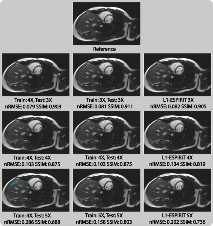
Selected cardiac images reconstructed with different testing/training acceleration factor settings in the proposed PI‐CNN network. [Color figure can be viewed at wileyonlinelibrary.com]
Figure 7 depicts the reconstruction results of prospectively undersampled data from GRAPPA, L1‐ESPIRiT and the proposed PI‐CNN network. We observed performance of the three reconstructions that was similar to the retrospectively study. GRAPPA reconstruction suffered from a high noise level, and L1‐ESPIRiT resulted in residual aliasing artifacts for certain case (blue arrows). On the other hand, the PI‐CNN network was able to produce much cleaner reconstruction and was less prone to remaining artifacts.
Figure 7.
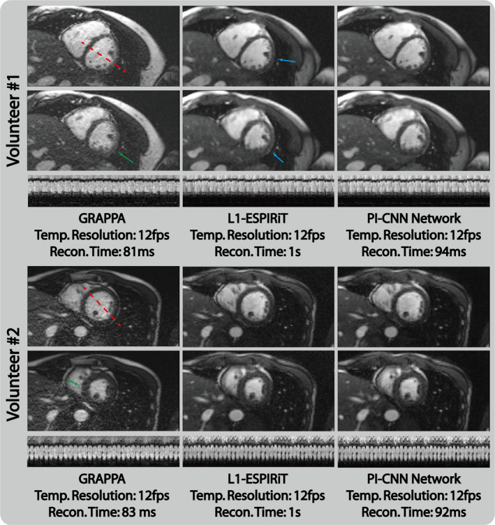
Reconstruction results of prospectively fourfold undersampled data from GRAPPA, L1‐ESPIRiT and the proposed parallel imaging and convolutional neural network (PI‐CNN) network. GRAPPA reconstruction has high noise level that results in poor visualization of the myocardium (green arrows). L1‐ESPIRiT reconstruction has a small residual aliasing artifact (blue arrows) in certain cases. Reconstructions from the proposed PI‐CNN network have less undersampling artifacts and an improved single to noise ratio. [Color figure can be viewed at wileyonlinelibrary.com]
Figure 8 demonstrates the advantage of the proposed method in single to noise ratio (SNR) limited scenario and its generalization capacity in patient cases. For both healthy volunteers and tumor patients, the linear reconstruction GRAPPA suffered from high noise level due to the poor conditioning of the system matrix in low SNR situation. L1‐ESPIRiT was able to reconstruct cleaner images but still has visible noise compared with the reference image. The proposed method, however, was able to reconstruct high quality images with well‐delineated tumor regions (blue, yellow, and red arrows). The reconstructed images also had a much lower noise floor and were comparable to the fully sampled reference. Quantitative measurements shown in Table I also confirm these observations.
Figure 8.
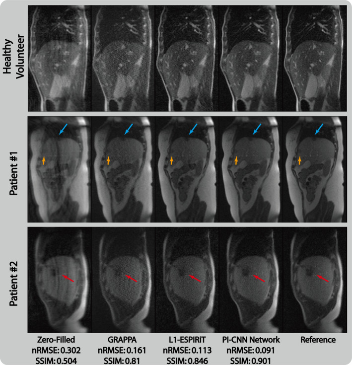
Comparison of different reconstruction strategies at threefold acceleration factor for sagittal view abdominal acquisitions at 0.35T low‐field environment. From left to right, each column represents selected frame reconstructed with zero‐filling, GRAPPA, L1‐ESPIRiT, proposed parallel imaging and convolutional neural network and reference, respectively. [Color figure can be viewed at wileyonlinelibrary.com]
The single‐coil–based network and proposed network, as well as the GRAPPA method are all compatible with on‐the‐fly reconstruction. Reconstruction time on eight cores and single GPU was 28 ms/frame for the single‐coil–based network, 46–108 ms/frame for proposed method depends on coil number, and 76–95 ms/frame for GRAPPA including calibration weight calculation. L1‐ESPIRiT with spatial wavelet constraint, on the other hand, took 1.2–1.4 s to reconstruct each frame.
4. Discussion
This work demonstrates the feasibility of using a PI and CNN combined network to perform low‐latency reconstruction on accelerated real‐time acquisitions. By taking advantage of an interleaved PI and CNN reconstruction, the network, once trained, is capable of reconstructing 2D images within tens of milliseconds and will likely enable on‐the‐fly reconstruction for high spatial and high temporal resolution real‐time MRI. In particular, we demonstrated that the PI‐CNN network is superior to both previously proposed single‐coil–based network32 and L1‐ESPIRiT47 at fourfold acceleration in 1.5 T for real‐time cardiac imaging. Comparison with L1‐ESPIRiT and clinical available GRAPPA reconstructions at SNR‐limited 0.35 T environment for real‐time abdominal imaging also shows the improved performance of proposed PI‐CNN network with threefold acceleration.
Previous literature in deep learning‐based MR image reconstruction30, 31, 32, 33 only shows the feasibility of reconstruction with single‐coil data and lacks a clear demonstration of how the clinical multiple‐coil data are handled. Compared to the selected single‐coil–based network used in this work, the proposed PI‐CNN network includes multicoil information to allow the network to better de‐alias the artifact‐contaminated zero‐filled input image. Given the same amount of training data and number of epochs, we believed the improved results of the proposed method come from a faster convergence and a smaller gap between the training‐testing errors (i.e., less overfitting), all resulting from the fact that more (multicoil) information is included in the PI‐CNN network.
The overfitting issue has always been a concern for learning‐based methods, especially with a training dataset of a relatively small size. To alleviate this, the proposed PI‐CNN network utilized a cascaded structure that interleaves the CNN layer and PI‐DC layer to constrain the size of the receptive field for each layer. The benefit of such a strategy can be clearly seen from Fig. 3. We also carefully choose the parameters related to the network design (, , ) that satisfies our application needs, which is essentially a trade‐off between model complexity and training efficiency. With increased model complexity (larger , , ), the network may be capable of delineating finer structures and removes stronger aliasing artifacts, but requires more training data and longer computation time. With increased training efficiency (smaller , , ), the network converges much quicker and needs less training data, but it will perform poorly when the undersampling factor increases. With the current setup (, , ), our experiments show that the proposed network can recover high‐quality images with less than 100 ms from moderate undersampled images.
Compared with the conventional CS approaches, the proposed learning‐based PI‐CNN network offers two distinct advantages for image reconstruction. First, CS methods usually require the selection of specific sparsifying transform(s) as regularization term(s) to constrain the solution space for the underdetermined problem, which is not a trivial task. Using the learning‐based approach allows the network to adapt its kernels to the underlying features of the image and artifacts automatically and requires minimal human interaction. Based on criteria given by the loss function, the training process optimally adjusts the convolutional kernels such that the output matches well with the reference. However, such data‐driven–based adaption from the training process can also limit the way that a learned network is used for reconstruction. As shown in Fig. 6, if the severity of aliasing artifacts is drastically different between the training and application stages, learning‐based PI‐CNN network performs inferior to the CS approach. Fortunately, recent research results have highlighted the potential of transfer learning45 to handle this training‐application mismatch. Its applicability to our proposed PI‐CNN network warrants future study. Second, CS reconstruction usually requires long reconstruction time since every reconstruction is treated as an individual optimization problem. On the contrary, the learning‐based PI‐CNN network offloads the computational expensive optimization process offline and precalculates the network parameters. Once the parameters are determined, the application to new data is extremely fast since no optimization is needed.
Our study shows that the proposed network can learn the general and global mapping from undersampled aliased image to reference image, using different sampling patterns with fixed undersampling factor during the training. This suggests that a fixed aliasing pattern or strong incoherence is not required, although more incoherent aliasing from trajectories such as radial sampling might be helpful at a higher undersampling factor. To further improve the network, one may pretrain the network with various undersampling masks, and fine tune it with a fixed pattern that will be finally used in the prospective study. Furthermore, jointly training the undersampling mask and aliased image for reconstruction may provide further improvement.
In the proposed PI‐CNN network, we utilized the multicoil information through an interleaved PI‐DC layer, which is essentially solving a parallel image problem with precalculated sensitivity maps. Alternatively, the multicoil data can be input into the network directly, and let the network itself to learn the implicit relationship between coils. As shown in a recent work (AUTOMAP),35 a general manifold approximation can be learned to map the acquired k‐space data directly to image domain, which in essence replaced the entire image reconstruction process with a knowledge‐free training network. Similarly, such a network can be employed to map multicoil k‐space data directly to single image without explicitly using the parallel imaging information. This could be better than the proposed approach which uses the coil sensitivity explicitly, but will greatly increase the network size and requires more processing such as data shuffling to prevent the network from learning a fixed coil arrangement.
In the low‐field abdominal imaging experiment, we incorporated patient cases to demonstrate the generalization capability of the proposed network. We ascribe the high‐quality reconstruction on patient data partly due to the fact that we incorporate k‐space data into the network and enforce the consistency repeatedly. This allows the network to capture the unseen features, including the pathology‐related features, during the application stage. However, since there is no clear idea what exactly the convolutional kernels represent in a learned network, the capacity of the proposed network to handle more complicated pathology cases remains undefined and warrants further investigation.
5. Conclusion
In conclusion, by taking advantage of multicoil information and convolutional neural network, a PI‐CNN reconstruction network has been successfully implemented and evaluated in both cardiac and abdominal real‐time imaging on retrospective and prospective data. Better image quality was achieved using the proposed PI‐CNN network than a single‐coil–based reconstruction network, L1‐ESPIRiT and GRAPPA on moderate 3X–4X acceleration. In terms of reconstruction speed, the proposed method can achieve less than 100‐ms reconstruction for clinical multicoil data, which implies its potential of real‐time reconstruction for real‐time imaging applications. A limitation of our study is that we developed and evaluated our technique only in a small number of subjects. A larger validation study would be appropriate to show the clinical utility in various patient populations.
Funding
NIH 1R01HL127153, Siemens Medical Solutions.
References
- 1. Narayanan S, Nayak K, Lee S, Sethy A, Byrd D. An approach to real‐time magnetic resonance imaging for speech production. J Acoust Soc Am. 2004;115:1771–1776. [DOI] [PubMed] [Google Scholar]
- 2. Bresch E, Kim Y‐C, Nayak K, Byrd D, Narayanan S. Seeing speech: capturing vocal tract shaping using real‐time magnetic resonance imaging. IEEE Sign Process Mag. 2008;25:123–132. [Google Scholar]
- 3. Weiger M, Pruessmann KP, Boesiger P. Cardiac real‐time imaging using SENSE. Magn Reson Med. 2000;43:177–184. [DOI] [PubMed] [Google Scholar]
- 4. Shankaranarayanan A, Simonetti OP, Laub G, Lewin JS, Duerk JL. Segmented k‐space and real‐time cardiac cine MR imaging with radial trajectories. Radiology. 2001;221:827–836. [DOI] [PubMed] [Google Scholar]
- 5. Wintersperger BJ, Nikolaou K, Dietrich O, et al. Single breath‐hold real‐time cine MR imaging: improved temporal resolution using generalized autocalibrating partially parallel acquisition (GRAPPA) algorithm. Eur Radiol. 2003;13:1931–1936. [DOI] [PubMed] [Google Scholar]
- 6. Cox RW, Jesmanowicz A, Hyde JS. Real‐time functional magnetic resonance imaging. Magn Reson Med. 1995;33:230–236. [DOI] [PubMed] [Google Scholar]
- 7. Christopher deCharms R. Applications of real‐time fMRI. Nat Rev Neurosci. 2008;9:720. [DOI] [PubMed] [Google Scholar]
- 8. Holsinger AE, Wright RC, Riederer SJ, Farzaneh F, Grimm RC, Maier JK. Real‐time interactive magnetic resonance imaging. Magn Reson Med. 1990;14:547–553. [DOI] [PubMed] [Google Scholar]
- 9. Busch M, Bornstedt A, Wendt M, Duerk JL, Lewin JS, Grönemeyer D. Fast, “real time” imaging with different k‐space update strategies for interventional procedures. J Magn Reson Imaging. 1998;8:944–954. [DOI] [PubMed] [Google Scholar]
- 10. Pruessmann KP, Weiger M, Scheidegger MB, Boesiger P. SENSE: sensitivity encoding for fast MRI. Magn Reson Med. 1999;42:952–962. [PubMed] [Google Scholar]
- 11. Griswold MA, Jakob PM, Heidemann RM, et al. Generalized autocalibrating partially parallel acquisitions (GRAPPA). Magn Reson Med. 2002;47:1202–1210. [DOI] [PubMed] [Google Scholar]
- 12. Lustig M, Donoho D, Pauly JM. Sparse MRI: the application of compressed sensing for rapid MR imaging. Magn Reson Med. 2007;58:1182–1195. [DOI] [PubMed] [Google Scholar]
- 13. Gamper U, Boesiger P, Kozerke S. Compressed sensing in dynamic MRI. Magn Reson Med. 2008;59:365–373. [DOI] [PubMed] [Google Scholar]
- 14. Block KT, Uecker M, Frahm J. Undersampled radial MRI with multiple channels: iterative image reconstruction using a total variation constraint. Magn Reson Med. 2007;57:1086–1098. [DOI] [PubMed] [Google Scholar]
- 15. Heywang‐Köbrunner SH, Heinig A, Pickuth D, Alberich T, Spielmann RP. Interventional MRI of the breast: lesion localisation and biopsy. Eur Radiol. 2000;10:36–45. [DOI] [PubMed] [Google Scholar]
- 16. Mutic S, Dempsey JF. The ViewRay system: magnetic resonance–guided and controlled radiotherapy. Sem Radiat Oncol. 2014;24:196–199. [DOI] [PubMed] [Google Scholar]
- 17. Feng L, Srichai MB, Lim RP, et al. Highly accelerated real‐time cardiac cine MRI using k–t SPARSE‐SENSE. Magn Reson Med. 2013;70:64–74. [DOI] [PMC free article] [PubMed] [Google Scholar]
- 18. Nayak KS, Pauly JM, Kerr AB, Hu BS, Nishimura DG. Real‐time color flow MRI. Magn Reson Med. 2000;43:251–258. [DOI] [PubMed] [Google Scholar]
- 19. Uecker M, Zhang S, Voit D, Karaus A, Merboldt KD, Frahm J. Real‐time MRI at a resolution of 20 ms. NMR Biomed. 2010;23:986–994. [DOI] [PubMed] [Google Scholar]
- 20. Lingala SG, Zhu Y, Lim Y, et al. Feasibility of through‐time spiral generalized autocalibrating partial parallel acquisition for low latency accelerated real‐time MRI of speech. Magn Reson Med. 2017;78:2275–2282. [DOI] [PMC free article] [PubMed] [Google Scholar]
- 21. Seiberlich N, Lee G, Ehses P, Duerk JL, Gilkeson R, Griswold M. Improved temporal resolution in cardiac imaging using through‐time spiral GRAPPA. Magn Reson Med. 2011;66:1682–1688. [DOI] [PMC free article] [PubMed] [Google Scholar]
- 22. Borisch E, Grimm R, Rossmann P, Haider C, Riederer S. Real‐time high‐throughput scalable MRI reconstruction via cluster computing. In: Proceedings of 16th Annual Meeting of ISMRM, Toronto, Canada; 2008:1492.
- 23. Sorensen TS, Atkinson D, Schaeffter T, Hansen MS. Real‐time reconstruction of sensitivity encoded radial magnetic resonance imaging using a graphics processing unit. IEEE Trans Med Imaging. 2009;28:1974–1985. [DOI] [PubMed] [Google Scholar]
- 24. Majumdar A, Ward RK, Aboulnasr T. Compressed sensing based real‐time dynamic MRI reconstruction. IEEE Trans Med Imaging. 2012;31:2253–2266. [DOI] [PubMed] [Google Scholar]
- 25. Jackson JI, Meyer CH, Nishimura DG, Macovski A. Selection of a convolution function for Fourier inversion using gridding. IEEE Trans Med Imaging. 1991;10:473–478. [DOI] [PubMed] [Google Scholar]
- 26. Ravishankar S, Bresler Y. MR image reconstruction from highly undersampled k‐space data by dictionary learning. IEEE Trans Med Imaging. 2011;30:1028–1041. [DOI] [PubMed] [Google Scholar]
- 27. Krizhevsky A, Sutskever I, Hinton GE. ImageNet classification with deep convolutional neural networks. Proc Adv Neural Inf Process Syst. 2012;1097–1105.
- 28. Xie J, Xu L, Chen E. Image denoising and inpainting with deep neural networks. Proc. Adv. Neural Inf. Process. Syst. 2012;341–349.
- 29. Dong C, Loy CC, He K, Tang X. Image super‐resolution using deep convolutional networks. IEEE Trans Pattern Anal Mach Intell. 2015;38:295–307. [DOI] [PubMed] [Google Scholar]
- 30. Wang S, Su Z, Ying L, et al. Accelerating magnetic resonance imaging via deep learning. In: IEEE13th International Symposium on Biomedical Imaging (ISBI), Prague;2016:514–517. [DOI] [PMC free article] [PubMed]
- 31. Yang Y, Sun J, Li H, Xu Z. Deep ADMM‐Net for compressive sensing MRI. In: Lee DD, Sugiyama M, Luxburg UV, Guyon I, Garnett R, eds. Advances in Neural Information Processing Systems (NIPS). New York: Curran Associates, Inc.; 2016:10–18. [Google Scholar]
- 32. Schlemper J, Caballero J, Hajnal JV, Price A, Rueckert D. A deep cascade of convolutional neural networks for MR image reconstruction. arXiv:1703.00555 preprint; 2017. [DOI] [PubMed]
- 33. Hyun CM, Kim HP, Lee SM, Lee S, Seo JK. Deep learning for undersampled MRI reconstruction. arXiv: 1709.02576 preprint; 2017. [DOI] [PubMed]
- 34. Hammernik K, Klatzer T, Kobler E, et al. Learning a variational network for reconstruction of accelerated MRI data. Magn Reson Med. 2018;79:3055–3071. [DOI] [PMC free article] [PubMed] [Google Scholar]
- 35. Zhu B, Liu JZ, Cauley SF, Rosen BR, Rosen MS. Image reconstruction by domain‐transform manifold learning. Nature. 2018;555:487–492. [DOI] [PubMed] [Google Scholar]
- 36. Lv J, Chen K, Yang M, Zhang J, Wang X. Reconstruction of undersampled radial free‐breathing 3D abdominal MRI using stacked convolutional auto‐encoders. Med Phys. 2018;45:2023–2032. [DOI] [PubMed] [Google Scholar]
- 37. Yao H, Dai F, Zhang D, Ma Y, Zhang S, Zhang Y, DR2 –NET: Deep residual reconstruction network for image compressive sensing. arXiv: 1702.05743; 2017.
- 38. Yang Y, Sun J, Li H, Xu Z. ADMM‐CSNet: a deep learning approach for image compressive sensing. IEEE Trans Pattern Anal Mach Intell. 2018;1–1. 10.1109/TPAMI.2018.2883941 [DOI] [PubMed] [Google Scholar]
- 39. Zhu J‐Y, Krähenbühl P, Shechtman E, Efros AA. Generative visual manipulation on the natural image manifold. In: Computer Vision – ECCV 2016. Cham, Switzerland: Springer; 2016:597–613. [Google Scholar]
- 40. Yeh RA, Chen C, Lim TY, Schwing AG, Hasegawa‐Johnson M, Do MN.Semantic image inpainting with deep generative models. https://arxiv.org/abs/1607.07539; 2016.
- 41. Sønderby CK, Caballero J, Theis L, Shi W, Huszár F. Amortised MAP inference for image super‐resolution. arXiv:1610.04490; 2016.
- 42. Ledig C, Theis L, Huszar F, et al. Photo‐realistic single image super‐resolution using a generative adversarial network. arXiv:1609.04802; 2016.
- 43. Mardani M, Gong E, Cheng JY, et al. Deep generative adversarial neural networks for compressive sensing MRI. IEEE Trans Med Imaging. 2019;38:167–179. [DOI] [PMC free article] [PubMed] [Google Scholar]
- 44. Yang G, Yu S, Dong H, et al. DAGAN: Deep de‐aliasing generative adversarial networks for fast compressed sensing MRI reconstruction. IEEE Trans Med Imaging. 2018;37:1310–1321. [DOI] [PubMed] [Google Scholar]
- 45. Dar SUH, Cukur T. A Transfer‐Learning Approach for Accelerated MRI using Deep Neural Networks. arXiv: 1710.02615; 2017. [DOI] [PubMed]
- 46. Han Y, Yoo J, Kim HH, Shin HJ, Sung K, Ye JC. Deep learning with domain adaptation for accelerated projection‐reconstruction MR. Magn Reson Med. 2018;80:1189–1205. [DOI] [PubMed] [Google Scholar]
- 47. Uecker M, Lai P, Murphy MJ, et al. ESPIRiT‐an eigenvalue approach to autocalibrating parallel MRI: where SENSE meets GRAPPA. Magn Reson Med. 2014;71:990–1001. [DOI] [PMC free article] [PubMed] [Google Scholar]
- 48. Kulkarni K, Lohit S, Turaga P, Kerviche R, Ashok A. ReconNet: Non‐iterative reconstruction of images from compressively sensed random measurements. IEEE International Conference on Computer Vision and Pattern Recognition (CVPR); 2016.
- 49. Kelly B, Matthews TP, Deep Anastasio MA.Learning‐Guided Image Reconstruction from Incomplete Data. arXiv: 1709.00584 preprint; 2017.
- 50. Hammernik K, Knoll F, Sodickson D, Pock T.L2 or not L2: Impact of Loss Function Design for Deep Learning MRI Reconstruction. In: Proceedings of 25th Annual Meeting of ISMRM, Honolulu, Hawaii, USA; 2017:687.
- 51. Zhao H, Gallo O, Frosio I, Kautz J. Loss functions for image restoration with neural networks. IEEE Trans Comput Imaging. 2017;3:47–57. [Google Scholar]
- 52. LeCun YA, Bottou L, Orr GB, Muller KR. Efficient backprop. In: Neural Networks: Tricks of the Trade. Berlin: Springer; 2012:9–50. [Google Scholar]
- 53. He K, Zhang X, Ren S, Sun J. Delving deep into rectifiers: Surpassing human level performance on imagenet classification. In: Proceedings of the IEEE International Conference on Computer Vision; 2015:1026–1034.
- 54. Kingma DP, Ba JL. Adam: a method for stochastic optimization. Int Conf Learn Represent. 2015;2015:1–15. [Google Scholar]
- 55. Uecker M, Ong F, Tamir J, Bahri D, Virtue P, Cheng JY, Zhang T, Berkeley LM.Advanced Reconstruction Toolbox, Annual Meeting ISMRM, Toronto 2015. In: Proc. Intl. Soc. Mag. Reson. Med 23;2486; 2015.
- 56. Wang Z, Bovik AC, Sheikh HR, Simoncelli EP. Image quality assessment: from error visibility to structural similarity. IEEE Trans Image Process. 2004;13:600–612. [DOI] [PubMed] [Google Scholar]