Cohort Creation
As noted earlier, MAPLE incorporates four longitudinal cohorts and one stacked longitudinal cohort that combines three cycles of the CanCHEC. The CanCHEC cycles used individual data from the long form census questionnaire, which includes variables on socioeconomic status such education, income, marital status, ethnicity, immigration status, and employment status. Although some of these variables were measured differently during different census years, all variables were standardized to allow all CanCHEC cohorts to be stacked and the CanCHEC and mCCHS cohorts to be comparable.
1991 CanCHEC — 2.5 million subjects (after exclusions) over the age of 25 years who completed the 1991 long-form census linked to vital statistics, tax records, and cause of death from census day (June 4, 1991) to December 31, 2016, using methodology previously described in Wilkins and colleagues (2008) and Peters and colleagues (2013).
1996 CanCHEC — 3 million subjects (after exclusions) over the age of 25 years who completed the 1996 long- form census linked to vital statistics, tax records, and cause of death from census day (May 14, 1996) to December 31, 2016 (Christidis and colleagues 2018).
2001 CanCHEC — 3 million subjects (after exclusions) over the age of 25 years who completed the 2001 long- form census linked to vital statistics, tax records, and cause of death from census day (May 15, 2001) to December 31, 2016 (Pinault et al. 2017).
Stacked CanCHEC — 7.1 million subjects (after exclusions) over the age of 25 years who completed one of the three census long-form questionnaires. If the same respondents were included in more than one census year, later census year data were excluded to eliminate duplication of respondents in the sample. Duplicate respondents across census years were identified using records from the Statistics Canada’s Derived Record Depository, which compiles individual data on Canadians within a secure computing environment.
CCHS and mCCHS — 540,900 subjects over the age of 25 years who completed one of the CCHS panels (2001, 2003, 2005, 2007, 2008, 2009, 2010, 2011, or 2012), which are linked to vital statistics, tax records, and cause of death from day of survey completion to December 31, 2016 (Sanmartin et al. 2016). The CCHS is an annual nationally representative interview survey (Statistics Canada 2005). In addition to basic sociodemographic content, the CCHS also includes individual-level information on self-reported health status, such as BMI, and health behaviors, including diet, physical activity, smoking, and alcohol consumption.
Noninstitutionalized respondents to the long form questionnaire who lived in Canada were considered in scope for linkage (Pinault et al. 2016b). To create the cohorts, respondents were linked to death records and residential history through the Statistics Canada Social Data Linkage Environment (Statistics Canada 2017b), which creates linked population data files for social analysis. CCHS respondents were asked at the time of survey if they agreed to record linkage and data sharing, and 95.2% of respondents agreed. Linkage was approved by Statistics Canada and is governed by the Directive on Microdata Linkage. The process begins with linkage to the Derived Record Depository, a highly secure linkage environment comprised of a national dynamic relational database of basic personal identifiers. Survey and administrative data are linked to the Derived Record Depository using G-Link, a SAS-based generalized record linkage software that supports deterministic- and probabilistic-linkage techniques developed at Statistics Canada (Fellegi and Sunter 1969). A list of linked unique individuals was created through linkages that were either deterministic (matching records based on unique identifiers) or probabilistic (matching records based on nonunique identifiers such as names, sex, date of birth, and postal code and estimating the likelihood that records are referring to the same entity). Through this linkage, we obtained each respondent’s annual mailing address postal code (to account for residential mobility in analysis) from tax records. Respondents with no postal code history were excluded from the analysis because we were unable to assign air pollution estimates or neighborhood covariates. Team members received security clearance to conduct all data linkages and analyses at secure Research Data Centers operated by Statistics Canada. Data were anonymized and person-years were rounded to the nearest 100 to prevent individual identification.
Postal code history was not available for each person in every year of follow-up, either because they did not file a tax return or because there were gaps in administrative data. We imputed 2.1% of person-years of missing postal codes if they shared the first two characters (Finès et al. 2017; Pinault et al. 2017), for a total of 89.9% of person-years with a valid postal code after imputation. Person-years were then excluded if they did not have an assigned postal code.
Additional person-years were excluded if respondents immigrated to Canada less than 10 years prior to the survey date (9,364,400 excluded), age during the follow-up period exceeded 89 years (7,357,200 excluded), or postal codes could not be matched to an air pollution estimate (17,814,400), a Can-Marg value (25,613,100), or airshed (25,545,500). Note that these exclusion numbers overlap for many person-years. Finally, the air pollution exposures were based on a 10-year moving average with a one-year lag. Person-years were excluded if the air pollution estimate in a given year was based on fewer than 7 out of 10 years of data (21,751,800).
In stacking three cycles of the CanCHEC, a total of 149,301,100 person-years was available. Finally, to create the Stacked CanCHEC, repeated CanCHEC respondents were excluded, leading to a final number of 128,371,800 person-years for analyses. Person-years excluded because of missing data were associated with persons who: died during follow-up, were age 80–89 years at baseline, reported being a visible minority, reported Indigenous identity, were unemployed, lived in Northern communities, or lived in rural communities.
For the CCHS/mCCHS cohort, response rates varied by cycle (2000/2001 [Cycle 1.1], 84.7%; 2003 [Cycle 2.1], 80.7%; 2005 [Cycle 3.1], 78.9%; 2007–2008, 76.4%; 2009–2010, 72.3%; 2011–2012, 68.4%), as did the numbers of respondents who agreed to data linkage (2000–2001 [Cycle 1.1], n = 117,800 respondents; 2003 [Cycle 2.1], n = 112,900 respondents; 2005 [Cycle 3.1], n = 113,900 respondents; 2007–2008, n = 112,700 respondents; 2009–2010, n = 104,700 respondents; 2011–2012, n = 104,100 respondents). Of those who agreed to linkage, 95.2% were successfully linked to the Social Data Linkage Environment, with 99.8% of relevant deaths linked. There were 540,900 respondents in the cohort with up to 36 years of residential history occurring both before and after the survey date. This was transposed to a file of person-years from entry data to end of follow-up (n = 5,902,100). Of these, a number of person-years were excluded for various reasons (note that totals will exceed number of deleted person-years, given that more than one exclusion criteria may apply to a single person-year), as follows: immigrated to Canada less than 10 years before survey date (n = 541,600 person-years); age during follow-up period exceeded 89 years (n = 161,000); had no postal code (n = 5,009,900); could not be linked to air pollution values (n = 5,711,600); could not be linked to Can-MARG values (n = 7,668,000); could not be linked to census metropolitan area (CMA) or census agglomeration (CA) size (n = 4,800,600); could not be linked to airshed (n = 3,500); the 10-year moving average was informed by fewer than 7 years of exposure (n = 39,843); the person-year occurred after the subject death (n = 343,600). The total available person-years for analyses was 4,404,957 after all exclusions.
Analysis Approach
Linear Modeling
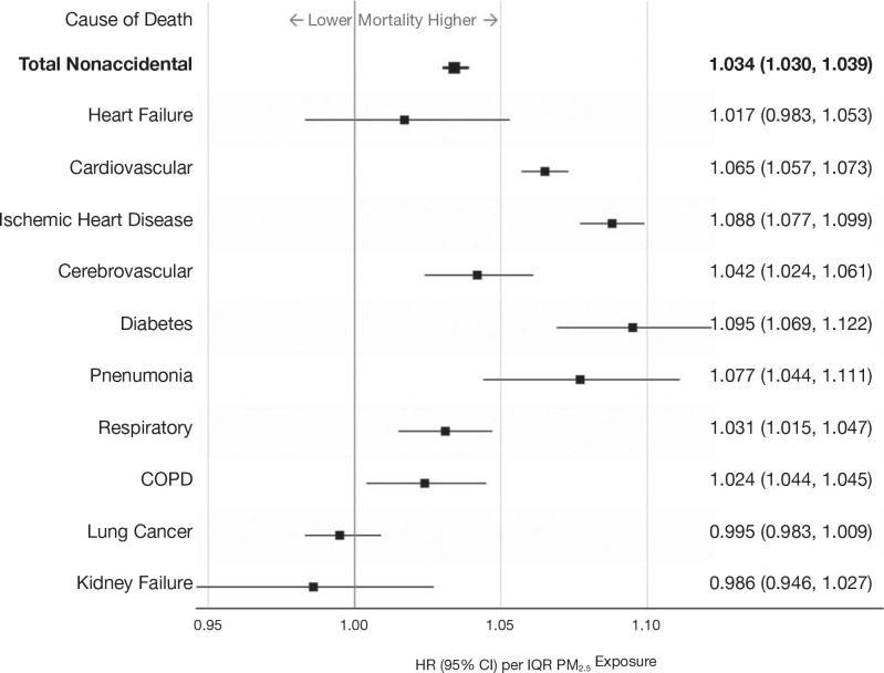
Our primary statistical model relating exposure to mortality was the Cox proportional hazards model. Participants were at least 25 years of age at the beginning of each cohort, and the time axis was the year of follow-up until 2016. Person-years before census year and after a subject’s death year were excluded from the analysis. Events were determined by year of death for nonaccidental and cause-specific mortality, using International Classification of Disease, 10th edition (ICD–10) codes. These include cardiovascular mortality (ICD-10 codes I10 to I69), cerebrovascular mortality (ICD-10 codes I60–I69), heart failure (ICD-10 codes I50.0, I50.1, I50.9), ischemic heart disease (ICD-10 codes I20–I25), diabetes (ICD-10 codes E10–E14), nonmalignant respiratory disease (ICD-10 codes J00–J99), COPD and associated conditions (ICD-10 codes J19–J46), pneumonia (ICD-10 codes J10–J18), lung cancer (ICD-10 codes C33–C34), and kidney failure (ICD-10 codes N18). The Cox model baseline hazard function was stratified by age (5-year groups), sex, and immigrant status. The Stacked CanCHEC and mCCHS were further stratified by census year or survey cycle. In this report we focus on the fully adjusted models introduced in the Phase 1 report. Specifically, models were adjusted for income adequacy quintile, visible minority status, Indigenous identity, educational attainment, labor-force status, marital status, occupation, and ecological covariates of community size, airshed, urban form, and four dimensions of Can-Marg (instability, deprivation, dependency, and ethnic concentration). Subject data were censored at 89 years of age, either at the beginning of each cohort or during follow-up, due to evidence from the 2011 Household Survey of an increased mismatch with increasing age between home address and tax return mailing address (Bérard-Chagnon 2017). We postulate that relatives of elderly people may have been completing their tax returns using a different address. Each of the three CanCHEC cohorts (1991, 1996, and 2001) were examined separately and then stacked to form a single cohort, which formed the basis of the majority of our analyses. Individuals who completed the subsequent long-form census questionnaires were removed, retaining only the first mention of the individual. Individuals who recurred in repeat CanCHEC cycles were identified using a key produced by the Derived Record Depository within Statistics Canada.
The primary exposure time window was a 10-year moving average assigned to the year prior to a given person-year, to ensure that exposures preceded the outcome event. Annual exposures were assigned by converting postal codes to geographic locations (i.e., latitudes and longitudes). However, some postal codes were missing, as not all subjects filed a tax return in each year. These missing postal codes were imputed based on available postal codes prior to and after missing years. Some postal codes could not be imputed with any accuracy and were set to missing. To estimate exposures, 7 years out of each 10-year period must have had available postal codes that were matched to air pollution estimates. We flagged missing person-years in the analytical file based on this requirement, and missing person-years were removed from the analysis. We required subjects to have filed tax returns 10 years prior to the cohort starting year (i.e., 1981 for the 1991 cohort, 1986 for the 1996 cohort, and 1991 for the 2001 cohort). An implication of this exposure-assignment protocol is that subjects must have been living in Canada 10 years prior to the beginning of their respective cohort’s follow-up period. We thus excluded all subjects who immigrated to Canada during the 10 years prior to their cohort enrollment. In earlier work, we evaluated the sensitivity of cause-specific HRs to immigration status and time since immigration. HRs for the association with cardiovascular and cerebrovascular mortality with PM2.5 were slightly but not significantly higher for immigrants relative to nonimmigrants in Canada, while no other differences were observed for other causes of death (Erickson et al. 2020). The implication from this work is that excluding recent immigrants was unlikely to introduce directional bias in our risk estimates.
Although several known and important risk factors for mortality were reported on the long-form census, many risk factors were not recorded, such as smoking habits, BMI, or diet. We addressed the influence of these risk factors on air pollution risk estimates using data from the CCHS. We pooled several cycles of the CCHS (mCCHS cohort) for simultaneous analysis of the shape of the concentration–response association between PM2.5 and nonaccidental mortality. The mCCHS analyses were stratified by CCHS cycle. We also examined several other causes of death, including cardiovascular mortality, cerebrovascular mortality, heart failure, ischemic heart disease, diabetes, nonmalignant respiratory disease, COPD and associated conditions, pneumonia, lung cancer, and kidney failure (ICD-10 codes described earlier).
We reported in the Phase 1 report a flattening of the all-cause mortality PM2.5 relationship at intermediate concentration ranges. Although concentration distributions overlap across airsheds, we utilized a newly available healthcare access measure to evaluate its potential relevance to the shape of the concentration–response relationship. The proximity to healthcare variable measures the closeness of a person’s home to local healthcare facilities: doctors and mental health specialists, dentists, offices of other health practitioners, outpatient care centers, and hospitals within a 3-kilometer network distance by car (Statistics Canada 2020). Proximity is measured by distance between the centroids of dissemination blocks which are an urban block or areas bounded by roads in a rural area. A simple gravity model weighs the number of nearby dissemination blocks containing healthcare facilities and the size of the services, by employment or revenue generation, and produces a normalized value from 0 to 1.
We attached this measure to the stacked cohort file through a postal code-dissemination block correspondence file produced by PCCF+. In cases where a postal code was not linked to a dissemination block, or if a dissemination block did not have a proximity estimate, we imputed the postal code proximity to healthcare value based on the mean values of similar, full postal codes, or more complete partial postal codes. After attaching the variable to the stacked cohort, we categorized all person-years according to quintile, and this five-category proximity variable was included in a restricted cubic spline analysis of nonaccidental death with 9-knots.
We split those who reside outside of a CMA–CA into those who live in rural (i.e., sparsely populated areas, 22,267,800 person-years) and nonrural areas (i.e., villages, small towns, 7,593,900 person-years), which can be assumed based on the second digit of a person’s postal code. We ran a 9-knot restricted cubic spline for nonaccidental death using our regular covariates and this slightly altered community size variable. The RCS curve did not change in a meaningful way.
Shape of the Association Between PM2.5 Exposure and Mortality
A quantitative characterization of the shape of the concentration–response relationship between outdoor PM2.5 concentrations and mortality can be useful for evaluating the health and economic benefits of proposed strategies to improve outdoor air quality. Cohort studies, such as those included in MAPLE are often used to determine this relationship. In such studies, information on major mortality risk factors such as age, sex, race, smoking, diet, exercise, and obesity are often included for each participant. Participants are assigned estimates of multiyear averages of outdoor concentrations of PM2.5 at or near their homes. These concentrations are then related to mortality using proportional hazard models adjusting for available information on other risk factors (Cox 1972) and HRs were reported with Wald CIs.
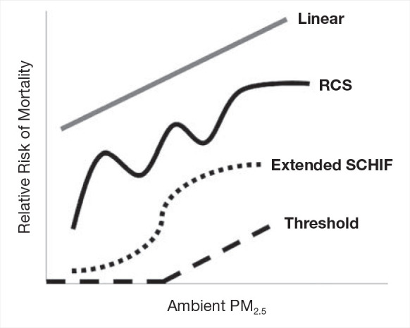
To assess the shape of air pollution–mortality relationships, we typically relate the concentration of PM2.5 to the logarithm of the hazard function, or instantaneous probability of death during follow-up, with a slope denoted by β. The hazard model (h) then has the form: logh(PM2.5) = β(PM2.5). This form of model has previously been used to estimate excess deaths from exposure to outdoor PM2.5 concentrations (U.S. EPA 2012). Some simple extensions of this linear model have been suggested, including logh(PM2.5) = βlog(PM2.5), where the logarithm of concentration is used (Crouse et al. 2012; Krewski et al. 2009). Nonlinear models have been extended to include nonparametric representations of the association using natural (Thurston et al. 2016) or restricted (Crouse et al. 2015) cubic splines. More complex extensions have included smoothing splines (Di et al. 2017). In these cases, several spline variables {sl (z), l = 1, . . ., L} are used to characterize the association:  for any concentration z, with the parameters {βl, l = 1, . . ., L} determining the magnitude. The spline variables take different shapes over different intervals of concentration. This local smoothing property allows for highly complex shapes to be modeled.
We have selected RCS to flexibly model the association between outdoor concentrations of PM2.5 and mortality (Harrell 2015). These regression-based splines require fewer computing resources compared with smoothing splines, a restriction that is necessary within the computing environment at Statistics Canada. The RCS has the form
for K ≥ 3 with
for K knot concentrations (λ1, . . ., λK). The RCS is linear below λ1 and above λK with continuous second derivatives at the K knots. The K-1 unknown parameters (β0, . . ., βK-2) are estimated within the Cox survival model framework by including (z,s1(z), . . ., sK(z)) as K-1 variables in the survival model. The analyst must specify the number and location of the knots. Knot locations are based on percentiles of the PM2.5 person-year distribution (Table 1). These are based on the recommendation given in the SAS macro lgtphcurv9 that we use to create the RCS variables and fit them with the Cox survival model (Li et al. 2011).
Let  be a K-1 by 1 vector of parameter estimates with corresponding covariance matrix V and let s(z) = (z, s1(z), . . ., sK-2(z))′. The estimate of the lnRCS(z) prediction is given by
with uncertainty in the estimate given by  We summarize the information obtained from the fitted RCS model by its mean prediction at any concentration z,
  , and its 95% confidence interval:
Selecting the Number of Knots
For all nonaccidental causes of death, we fit 16 RCS models based on 3 to 18 knots. We report the model predictions and 95% CIs in addition to two measures of fit: Akaike (AIC) and BIC, to examine the sensitivity of the shape of the PM2.5–mortality association to the number of knots.
Because of computing time limitations, for all other analyses we developed a supervised search routine to reduce the number of RCS models that were fit. Initially we fit RCS models with 5, 8, 11, and 14 knots and identified the number of knots with the lowest BIC value. Suppose this value is 11 knots. Then we fit another four models with 9, 10, 12, and 13 knots, toggling the number of knots above and below 11. We then identify the number of knots with the lowest BIC value among the 8 models run and select this as our final model, unless the best model is 16 knots (first selecting 14 knots) and then running 12, 13, 15, and 16 knots. In that case we run another four models with 17, 18, 19, and 20 knots. If the lowest BCI is in this range then we stop, if not we run multiple sets of four models until we reach a minimum BIC value. We used the log likelihood ratio test to compare the fit of the RCS vs the linear model.
Incorporation of Counterfactual Concentration
Natural cubic or smoothing splines are often used to describe the association between concentration and mortality. These splines are characterized by CIs increasing in width as concentrations deviate from the mean. RCS do not necessarily have this property. To represent the RCS predictions and their uncertainty in a manner similar to natural or smoothing splines we made the following adjustment:
Table 1.
Knot Location Person-Year Percentiles
| Knots |
Location |
| 3 |
5 50 95 |
| 4 |
5 35 65 95 |
| 5 |
5 27.5 50 72.5 95 |
| 6 |
5 23 41 59 77 95 |
| 7 |
2.5 18.3 34.2 50 65.8 81.7 98 |
| 8 |
1 15 29 43 57 71 85 99 |
| 9 |
2 14 26 38 50 62 74 86 98 |
| 10 |
2 12.7 23.3 34 44.7 55.3 66 76.7 87.3 98 |
| 11 |
2 11.6 21.2 30.8 40.4 50 59.6 69.2 78.8 88.4 98 |
| 12 |
2 10.7 19.5 28.2 36.9 45.6 54.4 63.1 71.8 80.5 89.3 98 |
| 13 |
2 10 18 26 34 42 50 58 66 74 82 90 98 |
| 14 |
9.39 16.8 24.2 31.5 38.9 46.3 53.7 61.1 68.5 75.9 83.2 90.6 98 |
| 15 |
2 8.9 15.7 22.6 29.4 36.3 43.1 50 56.9 63.7 70.6 77.4 84.3 91.1 98 |
| 16 |
2 8.4 14.8 21.2 27.6 34 40.4 46.8 53.2 59.6 66 72.4 78.8 85.2 91.6 98 |
| 17 |
2 8 14 20 26 32 38 44 50 56 62 68 74 80 86 92 98 |
| 18 |
2 7.6 13.3 18.9 24.6 30.2 35.9 41.6 47.2 52.8 58.5 64.1 69.8 75.4 81.1 86.7 92.4 98 |
with  Spline predictions are also often presented with the HR prediction equaling one at the lowest observed concentration, zmin. We include this property by transformatting the RCS predictions in the following manner:
Given this characterization, the lower confidence limit on the RCS prediction will be less than one at zmin. We identify the highest concentration, C, for which the lower confidence limit is less than one.
Relative-Risk Functions Suitable for Health Benefits Analysis
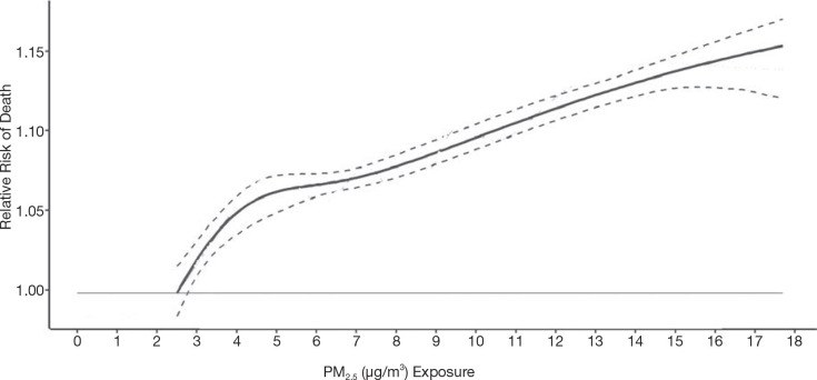
We present RCS mean predictions over the cohort concentration range and their 95% CIs. We set the mean prediction at the minimum concentration to one and a counterfactual concentration equaling the mean, at which the standard error (SE) of the prediction is zero. A characteristic of this formulation is that the width of the CIs increases as concentration deviates from the mean. We further identify the maximum concentration for which the lower confidence limit is less than one. The lower confidence limit on estimates of excess deaths will be less than zero for concentration ranges where the lower confidence limit on HR predictions is less than one. This calculation is based on a contrast between any concentration above the minimum and the minimum concentration, where it is assumed the HR at the minimum is one with zero uncertainty.
For a health benefits analysis, one is often interested in predicting the relative risk between any two concentrations, not just between a concentration above the minimum and the minimum itself. A benefits calculation incorporates the population attributable fraction (PAF), or proportion of total deaths attributable to any specific contrast in concentration, of the form:
where zC is a current concentration and zF < zC is a future predicted concentration under a specified air quality mitigation scenario. We therefore need to determine an estimate of  and its standard error. To do this we note that:
with standard error
Determining the difference in the log HR predictions between zC and zF only requires estimates of the respective predictions at each concentration,  , and
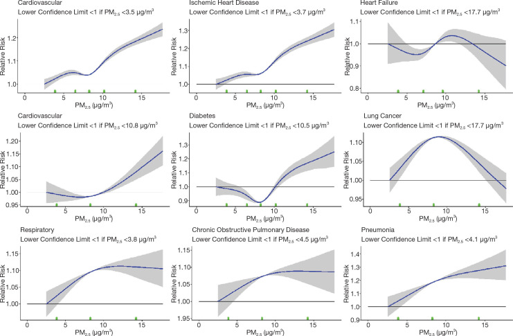
, and  , values that can be obtained from figures typically reported in publications such as those in Figures 13–19 in this report. However, determining
  requires estimates of each of the RCS variables (s0, . . ., sK-2) and the individual elements of the covariance matrix
  . Thus, the standard error of
  that could be obtained from the Figures 13–19 for example, is not sufficient to determine
  .
.
As an example application of risk predictions for health benefits analysis, the Global Burden of Disease 2019 (GBD 2020) uses a smoothing spline to characterize the magnitude, shape, and uncertainty in the association between air pollution concentrations and health outcomes within a Bayesian meta-analytic framework (GBD 2020). One thousand values are sampled from the posterior distribution of the spline coefficients. Using these values, 1,000 sets of the logarithm of relative-risk predictions are determined using a sequence of concentrations of interest. Then, 1,000 PAF values are created based on the difference in prediction between any two concentrations. We apply this method within our frequentist approach using the RCS by generating 1,000 realizations from a multivariate normal distribution with mean  and covariance matrix
  , denoted by ri = (r0,i, . . ., rK-2,i)′, i = 1, . . ., 1,000. We then construct: ri′(s(zC) – s(zF)), I = 1, . . ., 1,000 used to construct 1,000 estimates of the PAF(zC, zF) for the concentration contrast (zC, zF), a quantity necessary for health benefits analysis.
Extending the SCHIF
The best-fitting shape of the association estimated by splines may not be entirely suitable for risk assessment or health benefits analysis, due to potentially multiple variations in shape over different segments of the concentration distribution. That is, the spline maybe too wiggly even if it is constrained to be monotonically increasing (Pya and Wood 2015).
Our proposed approach to this challenge is to transform each of the 1,000 sets of predictions ri′s(zj), j = 0, . . ., J into an algebraic function that we suggest is suitable for benefits analysis. Our algebraic function is based on an extension of the SCHIF first proposed by Nasari and colleagues (2016) and then generalized as the Global Exposure Mortality Model (GEMM) by Burnett and colleagues (2018). It is given by
for j = 1, . . ., J; I = 1, . . ., 1,000. We fix the model prediction to ri′s(z0), the lnRCS value at z = z0, in order for our model to closely approximate the RCS predictions at very low concentrations. We denote this new model as eSCHIF. The second eSCHIF term was proposed by Burnett and colleagues (2018). We have added an additional term, the first eSCHIF term, to extend their model to additional shapes. In particular, this new formulation models confidence intervals of mean predictions that increase in width as deviation in concentration from their mean increase.
By setting the counterfactual to the mean concentration, the RCS CIs widen as concentrations deviate from the mean. The eSCHIF is thus capable of modeling such a structure, while the original SCHIF or GEMM are not. The eSCHIF can model near- linear, supralinear, sublinear, sigmoidal, and nonmonotonic shapes. A specific nonmonotonic shape of interest is when some of the RCS relative-risk predictions decline with concentration over lower concentrations and then increase with higher concentrations. This pattern results in PAF values less than zero.
eSCHIF Parameter Estimation
We use linear least squares to estimate the parameters (θi, γi) for specified values of (δ, α, μ, τ). We first generate uniform, U, sampling distributions for (δ, α, μ, τ) as:
v = zj - zo, the range in concentrations to be modeled over. We use these sampling distributions as a method to create a mesh of parameter values needed for our estimation routine. These sampling specifications also permit a wide range in shapes of interest.
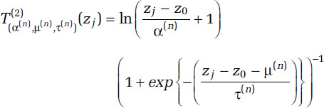
From these sampling distributions we generate a large number (1,000) of quadruples (δ(n), α(n), μ(n), τ(n)), for n = 1, . . ., 1,000 and then create two transformations of concentration (T(1) and T(2)) for each n and zj as
and
and include these two variables in a linear regression with the response ri′s(zj) - ri′s(z0), j = 0, . . ., J. We then identify the values of (δ(n), α(n), μ(n), τ(n)) that solicit the lowest log-likelihood value with corresponding estimates of (θi, γi) denoted by  . Let the corresponding values of (δ(n), α(n), μ(n), τ(n)) that minimize the log-likelihood be denoted by
Then the eSCHIF is characterized by
for j = 0, . . ., J; i = 1, . . ., 1,000.
The uncertainty distribution of PAF(zC, zF) based on the eSCHIF is obtained from the 1,000 values of
i = 1, . . ., 1,000, independent of ri′s(z0).
Incorporating Uncertainty in the Number and Location of RCS Knots
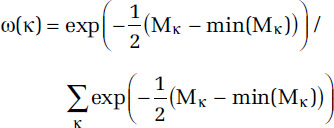
The shape and uncertainty of RCS predictions is governed, in part, by the number and placement of the knots. We characterize the uncertainty in number and placement of knots by first fitting RCS curves by a series of number of knots from 3 to 18. We then create an ensemble RCS estimate by first defining the ensemble weight ω(κ) with κ denoting the knot locations that define the RCS. Let Mκ denote a measure of fit associated with knots κ, then
(Buckland et al. 1997). We then form lnRCS model predictions over the exposure range by 0.1-μg/m3 increments, denoted by {z1, . . ., zN}, by simulating realizations proportionate to 1,000 × ω(κ). That is, the values of κ that yield better model predictions are more often represented in the 1,000 realizations. This approach incorporates uncertainty in both the number and location of the knots. To each of these 1,000 RCS realizations we fit the eSCHIF.
Standard Threshold Functions
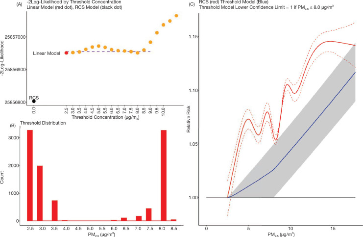
In addition to the eSCHIF for nonaccidental mortality we fit the standard threshold HR function:
where zρ = max (0, z - ρ), for threshold concentrations ρ = 2.5, 3.0, 3.5, . . ., 10.0. Let  denote the estimate of
  , its associated standard error; LLρ, the log-likelihood value; and
  the model ensemble weight (Buckland et al. 1997). We form model predictions by sampling 1,000 realizations of normal variates with mean
  and standard deviation
  with the sample size for each value of ρ proportionate to
  That is, the values of the threshold parameter ρ that represent better model predictions are more often represented in the 1,000 realizations. We graphically present the mean of the HR predictions among the 1,000 sets in addition to the 2.5 and 97.5 percentile values over the concentration range and identify the highest concentration, such that the 2.5 percentile value equals one.
Sensitivity Analyses
In addition to the main analyses described earlier, we conducted several sensitivity analyses using a similar modeling approach. These analyses were designed to further investigate observations reported in the MAPLE Phase 1 report. In most cases, we evaluated both linear Cox proportional hazards models as well as the nonlinear shape of the association between PM2.5 and mortality, described earlier, using fully adjusted models. In most cases, we focused on using the Stacked CanCHEC for these analyses, unless otherwise indicated.
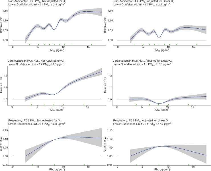
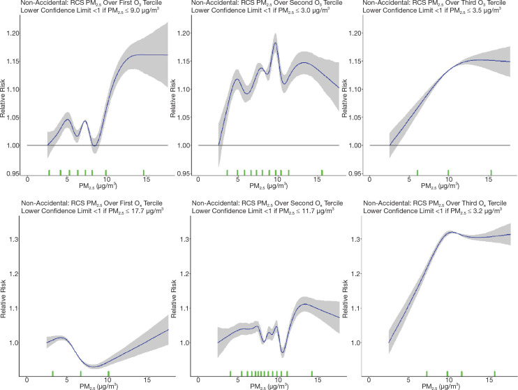
First, to further investigate the attenuation of PM2.5 HRs by O3 and Ox that we reported in the MAPLE Phase 1 report, we considered a series of joint two-pollutant models, incorporating both PM2.5 with O3 and PM2.5 with Ox, through linear and nonlinear models. Joint nonlinear models were fit using the number and position of knots obtained based on BIC model fit for each of the pollutants in the single-pollutant models. Similarly, we considered PM2.5 models within tertiles of O3 and Ox in both linear and nonlinear models for nonaccidental mortality.
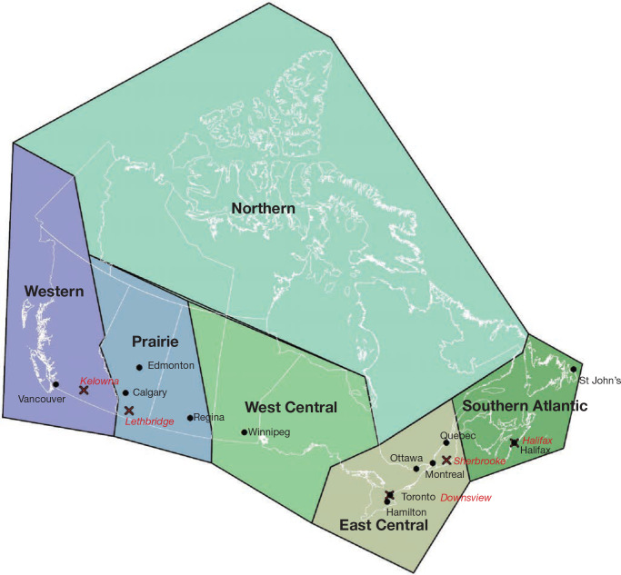
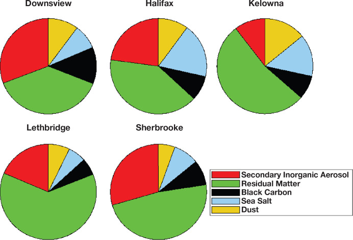
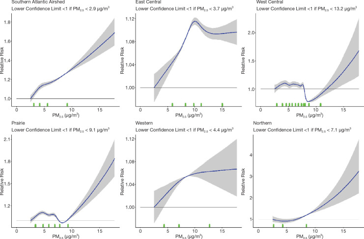
Next, we evaluated associations between nonaccidental mortality and PM2.5 within different regions of Canada. For this analysis, models were fitted by airshed, representing large areas of Canada (see Figure 3). This analysis was conducted to evaluate a flattening of the concentration–response relationship that we observed at midrange PM2.5 concentrations in the MAPLE Phase 1 report. We hypothesized that this may have reflected regional variation in the composition of the air pollution mixture at these levels or unmeasured regional variation in mortality risk factors. We additionally evaluated whether any observed regional variation in concentration–mortality relationships could be explained by differential regional representation of immigrants, Indigenous respondents, or healthy older persons who are lost to follow-up.
Further, we explored the potential effect of regional variation in access to healthcare as another factor that may have led to regional variation in the shape of the concentration– mortality relationship. In these analyses we evaluated separate models excluding immigrants, Indigenous respondents, and persons >80 years, 60–79 years, and >60 years, where immigrants and Indigenous respondents were removed, and where populations were restricted to specific age groups. To assess the sensitivity of concentration–mortality relationships to regional variation in access to healthcare, we included in models a new measure of the closeness of a census dissemination block to any census dissemination block with a healthcare facility within a driving distance of 3 kilometers. We further conducted analyses with 1-year age strata to assess potential residual confounding within the 5-year age strata in our main models.
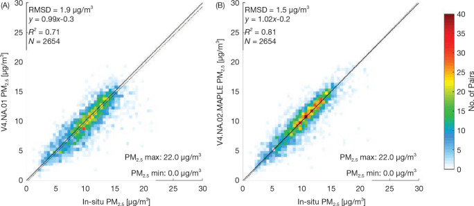
Finally, we evaluated model sensitivity to using different versions of applying PM2.5 exposure to the models. Different moving averages (3- vs. 10-year moving averages) were applied, as well as a comparison between the older version of the PM2.5 data (V4.NA.01) and the new version (V4. NA.02-MAPLE) (Appendix Tables A.6 and A.7; available on the HEI website).




 for any concentration z, with the parameters {βl, l = 1, . . ., L} determining the magnitude. The spline variables take different shapes over different intervals of concentration. This local smoothing property allows for highly complex shapes to be modeled.

 be a K-1 by 1 vector of parameter estimates with corresponding covariance matrix V and let s(z) = (z, s1(z), . . ., sK-2(z))′. The estimate of the lnRCS(z) prediction is given by
 We summarize the information obtained from the fitted RCS model by its mean prediction at any concentration z,
  , and its 95% confidence interval:

 Spline predictions are also often presented with the HR prediction equaling one at the lowest observed concentration, zmin. We include this property by transformatting the RCS predictions in the following manner:
 and its standard error. To do this we note that:
 , and
, and  , values that can be obtained from figures typically reported in publications such as those in
  requires estimates of each of the RCS variables (s0, . . ., sK-2) and the individual elements of the covariance matrix
  . Thus, the standard error of
  that could be obtained from the
  .
. and covariance matrix
  , denoted by ri = (r0,i, . . ., rK-2,i)′, i = 1, . . ., 1,000. We then construct: ri′(s(zC) – s(zF)), I = 1, . . ., 1,000 used to construct 1,000 estimates of the PAF(zC, zF) for the concentration contrast (zC, zF), a quantity necessary for health benefits analysis.

 . Let the corresponding values of (δ(n), α(n), μ(n), τ(n)) that minimize the log-likelihood be denoted by


 denote the estimate of
  , its associated standard error; LLρ, the log-likelihood value; and
  the model ensemble weight (Buckland et al.
  and standard deviation
  with the sample size for each value of ρ proportionate to
  That is, the values of the threshold parameter ρ that represent better model predictions are more often represented in the 1,000 realizations. We graphically present the mean of the HR predictions among the 1,000 sets in addition to the 2.5 and 97.5 percentile values over the concentration range and identify the highest concentration, such that the 2.5 percentile value equals one.








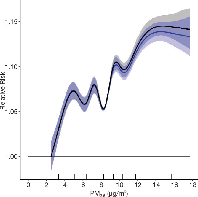
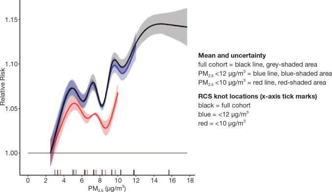
 to represent the mean predictions at a sequence of concentrations zj, j = 1, . . ., J and
  to represent the 95% CI to the average, 0.025, and 0.975 percentiles of ri′s(zj), i = 1, . . ., 1,000 for j = 0, . . ., J (


