Multiparametric 3-D analysis of bone and joint space width at the knee from weight bearing computed tomography

Abstract

Objective

Computed tomography (CT) can deliver multiple parameters relevant to osteoarthritis. In this study we demonstrate that a 3-D multiparametric approach at the weight bearing knee with cone beam CT is feasible, can include multiple parameters from across the joint space, and can reveal stronger relationships with disease status in combination.

Design

33 participants with knee weight bearing CT (WBCT) were analysed with joint space mapping and cortical bone mapping to deliver joint space width (JSW), subchondral bone plate thickness, endocortical thickness, and trabecular attenuation at both sides of the joint. All data were co-localised to the same canonical surface. Statistical parametric mapping (SPM) was applied in uni- and multivariate models to demonstrate significant dependence of parameters on Kellgren & Lawrence grade (KLG). Correlation between JSW and bony parameters and 2-week test-retest repeatability were also calculated.

Results

SPM revealed that the central-to-posterior medial tibiofemoral joint space was significantly narrowed by up to 0.5 mm with significantly higher tibial trabecular attenuation up to 50 units for each increment in KLG as single features, and in a wider distribution when combined (p<0.05). These were also more strongly correlated with worsening KLG grade category. Test-retest repeatability was subvoxel (0.37 mm) for nearly all thickness parameters.

Conclusions

3-D JSW and tibial trabecular attenuation are repeatable and significantly dependent on radiographic disease severity at the weight bearing knee joint not just alone, but more strongly in combination. A quantitative multiparametric approach with WBCT may have potential for more sensitive investigation of disease progression in osteoarthritis.

INTRODUCTION

Multiparametric imaging in osteoarthritis is usually considered the reserve of MRI, with measurement of T2 and T1rho half-life values, perfusion on dynamic contrast enhanced MRI, and cartilage morphology recognised as relevant to disease [1]. However, although of a different nature to MRI, multiple parameters can also be quantitatively derived from CT imaging, including bone mineral density, cortical bone thickness, cartilage thickness on arthrography, joint space width (JSW) on weight bearing, and shape [2–5].

In vivo techniques in the CT family (which include peripheral quantitative CT (pQCT), high resolution pQCT (HR-pQCT), multidetector helical CT, cone beam CT (CBCT), dual energy and spectral CT) are also used to measure multiple parameters from a single acquisition, for example with Karhula et al. in 2020 exploring subvoxel estimation of bone morphometrics from CBCT when compared to microCT and histological analysis [6]. Other studies recently have looked at simultaneous quantification of bone mineral density and cartilage thickness using contrast-enhanced HR-pQCT and CT [7,8].

Although there are recognised associations, the behaviour of bone in relation to developing osteoarthritis remains poorly understood, with one cross-modality study identifying subchondral bone plate differences between injured and contralateral non-injured knees with HR-pQCT but no difference in cartilage distribution on MRI [9]. Yet joint space narrowing and subchondral bone sclerosis are widely accepted markers of the osteoarthritic joint.

The evolving capabilities of CT present an opportunity to define its role in establishing relationships between the natural history of osteoarthritis and imaging features of disease, in particular those it can depict as well as or better than alternative modalities. If CT output could be harnessed appropriately, it may have potential to be a time- and cost-efficient alternative to MRI in assessing disease progression and a more sensitive and reliable modality than radiography in the setting of osteoarthritis research trials and the clinic, particularly noting that CBCT that has a much lower dose compared to traditional helical multidetector CT, in addition to weight bearing functionality.

Having already established that 3-D quantification with weight bearing CT (WBCT) might lead to greater sensitivity in detecting changes in JSW than radiography [4], CT might also be similarly used to assess the phenomenon of bony sclerosis that has been historically difficult to quantify. Here we revisit a previous analysis of JSW but now in combination with a new 3-D assessment of adjacent subchondral bone at the knee joint from a single WBCT acquisition. Our hypothesis was that a quantified 3-D multiparametric approach across the weight bearing knee joint was (i) feasible, (ii) would allow investigation into the correlation of these features, and (iii) might reveal stronger relationships with disease severity than single parameters alone. We also demonstrate the test-retest repeatability for all these parameters, an important metric to understand for their ability to detect meaningful change against day-to-day variations in imaging acquisition.

METHODS

Participants for this study were the same as the combined convenience groups from two separate knee WBCT studies performed between 2014 and 2018, as recently presented by Turmezei et al. [4]. The first convenience sample of simultaneous weight bearing CT images of both knees was from 23 individuals in the Multicenter Osteoarthritis Study from 2016 to 2018 who were involved in a prior study comparing WBCT with radiographic JSW[10]. Participants were recruited to the Multicenter Osteoarthritis Study, which had The University of Iowa institutional review board approval for demographic data collection (approval number 20003064) and WBCT image acquisition (approval number 201602741; all approved under FWA00003007). All participants provided informed consent prior to enrolment. The second convenience sample of simultaneous bilateral knee WBCT images included 10 individuals recruited between June and August of 2014 for another study looking at the test–retest repeatability of a different JSW measurement method [11]. For that study, The University of Iowa institutional review board approval (no. 201403723) was obtained in conjunction with informed oral consent from all participants.

Combined from both studies, there were 33 individuals who had both knees imaged simultaneously in a 20-degree fixed-flexion position with the same prototype commercial CBCT imaging system (LineUp; CurveBeam). The first visit imaging was used from the second sample in the statistical parametric mapping (SPM) study, with follow-up imaging for repeatability analysis having been performed at a second visit 2 weeks later. The Kellgren & Lawrence grade (KLG) breakdown for all 66 knees included in the analysis was KLG0 = 31, KLG1 = 12, KLG2 = 14, KLG3 = 7, and KLG4 = 2. All participants had knee joint positioning fixed by a lower limb positioner that held the feet externally rotated by 10°; a vertical plate that held the patellae and thighs in line with the tip of the great toes; and the anterior superior iliac spines’ and greater trochanters’ positions fixed for reliability within and between participants [12,13]. Imaging data were reconstructed with 0.37 mm isotropic voxels in a 200 × 350 mm axial field of view with 533 axial frames across the knee joint over a 20 cm scan range from at least the distal femoral diametaphysis to proximal tibial diametaphysis, and a standard bone kernel. The typical effective radiation dose for each examination was 0.024 mSv, with a volumetric CT dose index of 1.1 mGy and a dose-length product of 22 mGy · cm. This effective dose can be compared to 0.005 mSv for a plain radiograph set of the knee joint and an average US daily background exposure of 0.008 mSv: one WBCT acquisition is therefore roughly equivalent to 3 days of background radiation[14].

Imaging data sets were previously analysed using joint space mapping (JSM) as reported by Turmezei et al.[4]. In brief, after the distal femur is segmented from the axial imaging data, patches are cut from the femur bone surface object as guided by the shadow of the opposing tibial bone projected back on to the femoral surface. These joint space patches are the framework for the measurement of the distance between the joint bone surfaces (i.e. JSW) using a full-width half-maximum deconvolution of data sampled along a line at the normal to every vertex in the joint space patch mesh. The femoral and tibial articular bony surfaces are thus defined by JSM and contain the same relationship and connectivity of vertices as the original joint space patch mesh [4].

In this study, new analysis was performed to quantify subarticular bone thickness and trabecular attenuation at these femoral and tibial joint surface patches in 3-D using an endocortical algorithm implementation of cortical bone mapping (CBM) that allows measurement of subchondral, endocortical, and trabecular bone regions along a line at the normal to each vertex at the articular bone surface (Fig. 1) [15]. In this representation, trabecular attenuation is the CBM optimiser algorithm’s estimation of the average attenuation value of the bony trabecular network along the line of measurement beneath the joint surface.

Fig. 1.

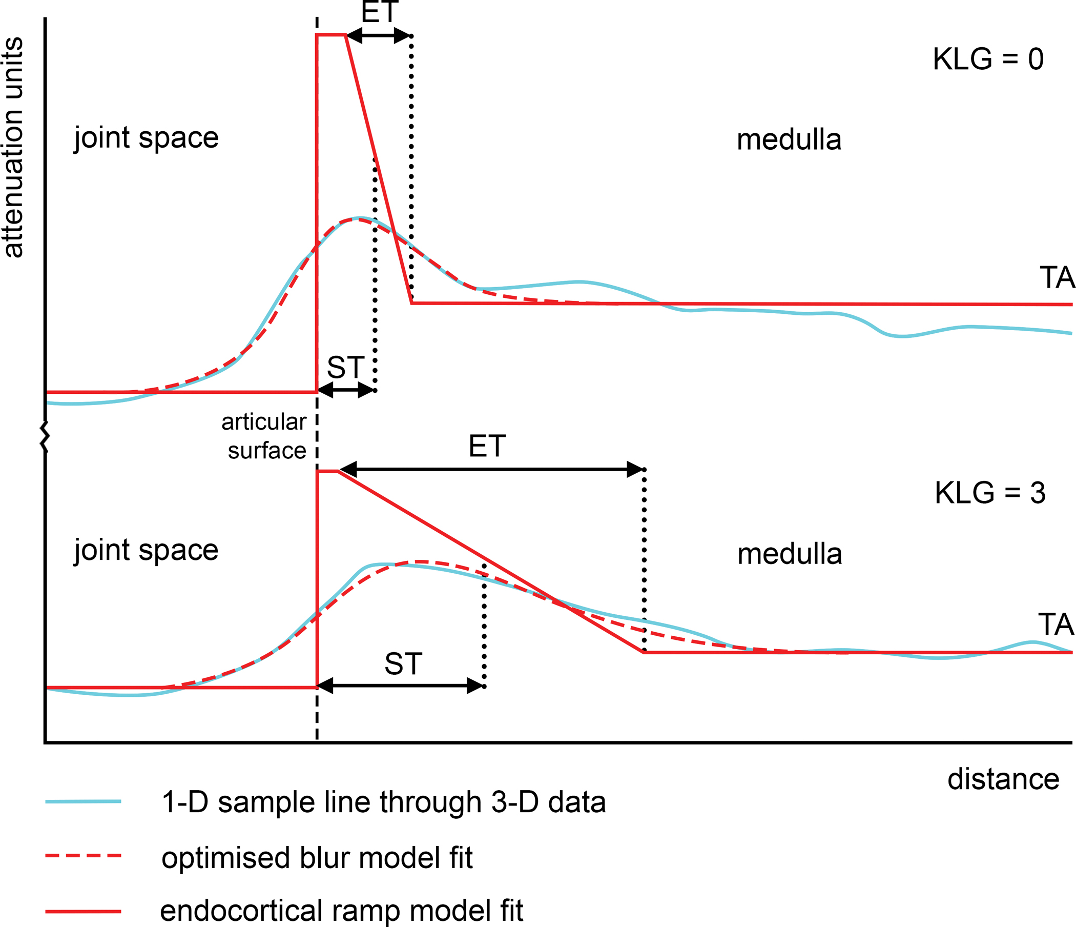
Endocortical CBM uses a ramp model to fit the tail-off from the cortex towards the medulla of the bone. Endocortical thickness (ET) is defined as the width of the ramp, while subchondral bone plate thickness (ST) is defined as the peak thickness plus half of the ramp. This means that the parameters are intrinsically correlated, but also that no specific depth region of interest is required to be pre-set. The overall 1-D line length was 30 mm, sampling from 10 mm outwards from the bone surface to 20 mm inwards. The top graph shows the optimised blur model fit (dashed red line) to the sampled attenuation value data (light blue line), with the ramp deconvolution model fit (solid red line) at a single tibial sample point for an individual from the study with KLG = 0 compared to an individual with KLG = 3 in the bottom graph.

Both JSM and CBM were performed using the free-to-download, in-house StradView software (version 6.13 [Graham Treece, Cambridge University]; https://mi.eng.cam.ac.uk/Main/StradView). The combination of these two techniques allows weight bearing JSW and the subarticular bony parameters of subchondral bone plate thickness (ST), endocortical bone thickness (ET), and trabecular attenuation (TA) at the distal femur (f) and proximal tibia (t) to be co-located vertex-by-vertex on each individual’s 3-D joint surface. After registration of the average joint surface (which we call the ‘canonical’ surface as a reasonable and realistic representation) to each individual’s surface, and then transfer of the multiparametric data from each individual onto this canonical, all data was then analysed and presented on the canonical model. All registrations and data transfer to the canonical were performed using the free-to-download, in-house software wxRegSurf (version 20 [Andrew Gee, Cambridge University]; https://mi.eng.cam.ac.uk/~ahg/wxRegSurf/).

Horn’s parallel analysis performed on the results of principal component analysis of the registration vectors showed that the first three shape modes were responsible for shape mode variation above background noise [16]. In order to look at the dependence of each parameter (fST = femoral subchondral thickness, fET = femoral endocortical thickness, fTA = femoral trabecular attenuation, tST = tibial subchondral thickness, tET = tibial endocortical thickness, tTA = tibial trabecular attenuation, and JSW) on KLG with SPM, a univariate general linear model was used with an experimental term of KLG (centrally graded in MOST) and confounding terms of age, body mass index, and the first three shape modes to control for effects of systematic misregistration [17,18]. A custom-scripted multivariate implementation of SPM was used to look at the co-dependence of each parameter pairs on the experimental term of KLG, again using the freely downloadable SurfStat package (Keith Worsley, McGill University; https://www.math.mcgill.ca/keith/surfstat/). Sex was not used in the model because of the correlation with the first shape mode (r = 0.80) that represented scale factor. Pearson’s correlation coefficient was also calculated vertex-wise on the canonical surface for each of the parameter pairs.

All 20 knees from the 10 individuals that were recruited to the test-retest repeatability study where used for measuring repeatability of all parameters, delivering bias, limits of agreement (LOA) adjusted to allow for more than one knee coming from one individual in the sample[19], and root mean square coefficient of variation (RMSCV) where possible, i.e. not with trabecular attenuation that has negative values. The process of spatially co-aligning data on the canonical surface to compare baseline and follow-up values has been previously described by Turmezei et al. in 2021 [4].

RESULTS

The mean ± SD age of participants at the time of imaging was 57.4 ± 7.2 years, with 23 women and 10 men in the study. All results are displayed on the canonical joint surface model, with an example of this model shown in Fig 2. displaying mean JSW from across the study at the right knee superimposed on the grey distal femur (viewed from below).

Fig. 2.

Example of mean JSW from across all 66 knees in the study shown in situ on the canonical knee joint surfaces (colour map) over a right distal femur (grey).

SPM revealed that the central-to-posterior medial tibiofemoral joint space was significantly narrowed by up to 0.5 mm with significantly higher tTA by up to 50 attenuation units for each increment in KLG (p<0.05) both as single features (Fig. 3, left) and in a wider distribution in combination with multivariate analysis (Fig. 3, right). A small patch at the medial aspect of the lateral joint space also showed significance for JSW alone and JSW/tTA in combination (p<0.05), suggesting that this is modelling medial tibiofemoral joint space loss with subchondral sclerosis along with medial shift of the femoral condyles with respect to the tibial plateau.

Fig. 3.

SPM results from univariate analysis (left column of maps) showing unmasked regions of significantly narrower joint space and greater tibial trabecular attenuation, which become larger in area when combined in the paired multivariate analysis (right column of maps). Joint space width is measured in mm and trabecular attenuation in attenuation units. The significance threshold for unmasked regions is p < 0.05, routinely the lower of the two colour scale bars, with masked non-significant values represented by the upper colour bar.

Note that the size of the significant regions of interest in the paired JSW-tTA parameter (multivariate) analysis are larger than for either single parameter, meaning that there are some points in the joint space that are only significantly dependent on KLG when parameters are combined. The percentage of the canonical joint space achieving the significance threshold by vertex count increased from a baseline of 16.1% (lateral/medial = 7.4%/23.6%) for JSW and 16.9% (0%/31.1%) for tTA to 33.8% (12.7%/51.6%) when JSW and tTA were combined: no other combinations showed such an increase for both parameters, evidencing the strength of their association. There were much smaller regions of significance for JSW and tTA in combination other parameters, but these were regarded as effects dominated by these already strongly significant single parameters, none of which showed any increase in percentage coverage value when in combination compared to the original single parameters. A full matrix of single and paired parameter SPM results by percentage of significant vertices is shown in Table 1, including the medial and lateral compartment breakdown.

Table 1.

A matrix of single parameter (along the diagonal) and paired parameter SPM results by % of significant vertices in the canonical patch, p < 0.05. The lateral/medial % split is shown in brackets. Any paired results in which there was an increase in percentage value compared to both single parameter results are emboldened. Single parameter cells are shaded in grey, pairs with JSW in white, pairs from the same side of the joint in orange, and across the joint space in purple.

%	JSW	fST	fET	fTA	tST	tET	tTA
JSW	16.1 (7.4/23.6)	4.3 (0/8.0)	6.3 (0/11.6)	6.8 (0/12.4)	4.6 (3.2/5.8)	4.8 (3.7/5.8)	33.8 (21.7/51.6)
fST	4.3 (8.0/0)	- (-/-)	- (-/-)	0.5 (0/0.9)	0.2 (0/0/4)	- (-/-)	14.7 (0/27.1)
fET	6.3 (0/11.6)	- (-/-)	- (-/-)	- (-/-)	- (-/-)	- (-/-)	15.9 (0/29.3)
fTA	6.8 (0/12.4)	0.5 (0/0.9)	- (-/-)	0.2 (0/0.4)	1.2 (0/2.2)	1.2 (0/2.2)	15.2 (2.1/26.2)
tST	4.6 (3.2/5.8)	0.2 (0/0/4)	- (-/-)	1.2 (0/2.2)	1.8 (0/1.0)	- (-/-)	11.3 (0/20.8)
tET	4.8 (3.7/5.8)	- (-/-)	- (-/-)	1.2 (0/2.2)	- (-/-)	0.5 (0/0.9)	10.6 (0/19.6)
tTA	33.8 (21.7/51.6)	14.7 (0/27.1)	15.9 (0/29.3)	15.2 (2.1/26.2)	11.3 (0/20.8)	10.6 (0/19.6)	16.9 (0/31.1)

Given theirs being the only stronger paired relationship demonstrated with SPM, for economy of space we show the mean values of the co-dependent factors of JSW and tTA and how they correlate across the joint space in the same KLG category divisions (Fig. 4). The mean distribution maps for all parameters are shown in Figs S1 and S2 broken down according to KLG < 2 (n=43) vs KLG = 2 (n=14) vs KLG > 2 (n=9) categories.

Fig. 4.

Mean JSW and tTA with their correlation map results also broken down KLG < 2 vs KLG = 2 vs KLG > 2.

Vertex-wise correlation maps in Fig. 4 show that JSW and tTA are more closely correlated with higher KLG category, with the percentage of vertices correlating at r > |0.50| increasing from 2%, to 11%, to 30% for KLG < 2, KLG = 2, and KLG > 2 respectively. This indicates stronger correlation of these two features with worsening radiographic disease, with larger JSW values in the lateral joint space linked to lower tibial trabecular attenuation values, suggesting widening with less sclerosis (or vice versa). There is a more heterogeneous relationship at the medial joint space, predominantly with smaller JSW values linked to larger attenuation values, suggesting narrowing with a mix of more and less sclerosis according to location (or vice versa).

Repeatability for each parameter is presented as average bias from across the whole joint space and best limits of agreement values in Table 2 and Table 3 respectively. Full tabulation of repeatability metrics by KLG category, including confidence intervals for limits of agreement and whole joint average root mean square coefficient of variation are included as supplementary Tables S1 to S7. This supplementary material also includes surface distribution maps by KLG category that allow regions to be identified on the joint surface where bias and limits of agreement performance are best (Figs S3 to S9). These visualisations demonstrate that there is variation in repeatability performance across the joint surface, in part due to noise from the small number of participants, but also often worse at the joint space margins where misalignment between baseline and follow-up values is likely to have greatest influence on error [20].

Table 2.

Average whole joint space bias for all parameters across grade categories

	KLG<2	KLG=2	KLG>2
JSW (mm)	0.00	0.03	0.06
fST (mm)	0.01	−0.01	0.01
fET (mm)	0.02	−0.02	0.02
fTA (AU)	−1.3	0.0	−1.7
tST (mm)	0.01	0.01	−0.04
tET (mm)	−0.01	0.01	−0.09
tTA (AU)	−0.5	−1.8	−7.8

Table 3.

Best limits of agreement for all parameters across grade categories and this, where possible, as a percentage of the mean joint surface parameter value.

	KLG<2	KLG=2	KLG>2ss
JSW (mm)	0.08 (1.7%)	0.40 (7.8%)	0.20 (4.0%)
fST (mm)	0.04 (5.6%)	0.05 (8.2%)	0.02 (3.3%)
fET (mm)	0.10 (12.2%)	0.10 (16.1%)	0.10 (18.5%)
fTA (AU)	11 (-)	11 (-)	6 (-)
tST (mm)	0.06 (4.9%)	0.10 (9.7%)	0.06 (6.3%)
tET (mm)	0.12 (8.2%)	0.12 (10.5%)	0.08 (8.4%)
tTA (AU)	15 (-)	20 (-)	13 (-)

Looking at the repeatability of thickness metric absolute values from Table 3, these are nearly all subvoxel (less than 0.37 mm) in magnitude apart from repeatability of JSW for the KLG = 2 category. This result appears to be anomalous but is in fact similar in percentage of the mean to many of the other thickness measures that achieve repeatability at best around or less than 10% of the mean measure, noting that JSW measures will be nearly one order of magnitude greater than bone thickness (e.g. 1 to 10 mm compared to 0.1 to 1 mm). It also highlights how relatively better the repeatability is for JSW in the KLG < 2 and > 2 categories. The exception to this is for fET, in which repeatability performance ranges from 12.2% in the KLG < 2 category up to 18.5% in the KLG > 2 category. Note that while attenuation values cannot be expressed as a percentage of the mean (because the attenuation scale has negative values), repeatability variations are nonetheless very small (between 6 and 20 attenuation units) when considering mean bone attenuation values across the joint space are around 300.

DISCUSSION

This study has shown it is possible to co-localise 3-D surface based multiparametric measurements across the weight bearing knee joint using cone beam CT (CBCT) imaging, specifically when analysing joint space width (JSW) and bony parameters such as subchondral plate thickness and trabecular attenuation. We have demonstrated the feasibility of multivariate significance testing in pairs and parameter correlations from both sides of the joint. As a trend, the most recognisable pattern in structural bone depicted by cortical bone mapping (CBM) was greater tibial and femoral subarticular bone thickness and attenuation measurements in the medial joint space with worse Kellgren & Lawrence grade (KLG) category, which could be taken as a quantitative correlate of subchondral sclerosis (Figs S1 and S2). This approach to evaluating subchondral bone with CT has been recognised as having potential for decades, with MRI also more recently having been used to analyse this feature [21,22]. As reported previously, joint space mapping (JSM) demonstrated greater narrowing of the medial joint space with worse KLG category [4], which is a staple feature in the radiographic assessment of osteoarthritis that can be expected to progress from −0.1 to 0.7 mm per year at the knee in those with radiographically established disease [23].

Yet while joint space narrowing and subchondral sclerosis are well-recognised elements of osteoarthritis, here we have demonstrated the 3-D co-localisation and quantification of correlation and combined significance testing for their dependence on disease status that should prompt further investigation of their combined strength as predictive parameters in future studies. Statistical parametric mapping (SPM) showed that combining JSW and tibial trabecular attenuation (tTA) in paired multivariate analysis increased the surface distribution of their dependence from around 16% to 31% of the joint space and nearly. This was the only parameter pairing to demonstrate strengthened dependence in this fashion. Stronger correlations between these two parameters were noted in individuals with worse radiological disease, but we also identified little or no correlation between them in a structurally healthy state (according to KLG<2). This suggests that JSW and tTA may become linked when structural disease is established, a relationship that could be explained by the development of subchondral bony sclerosis at sites of cartilage breakdown (or vice versa). This relationship needs further evaluation because the correlation we find in this exploratory study is both strongly positive and negative in the medial joint space. Previous investigation with MRI has shown that baseline subchondral sclerosis was not associated with future cartilage loss in the same knee compartment at either the femoral or tibial aspect [24], but our results suggest there is an association between joint space loss (whatever the cause) and increased tibial subchondral bone attenuation and, to a less widely distributed extent, subchondral bone plate and endocortical thickness. These relationships warrant further exploration. The fact that no femoral bony parameters met any substantial significance alone or in combination with JSW (Table 1) may be from underpowered analysis since a trend for increased femoral trabecular attenuation was identified with worsening KLG category (Fig. S1).

Repeatability results for thickness parameters were nearly all subvoxel (less than 0.37 mm) in value, demonstrating the ability of our 3-D algorithmic deblurring approach to deliver excellent repeatability, with best limits of agreement values nearly all less than 10% of the mean value, apart for fET. This can be explained by the algorithmic basis for determining the endocortical bone slope (Fig. 1) being more susceptible to slight variations in the optimisation process than for attenuation and JSW measures: because endocortical thickness values are most reliant on this slope, they can therefore be expected to be less repeatable in day-to-day measurement. Future exploration would therefore be of value into whether the endocortical ramp method is therefore the most appropriate to model subchondral bone at the knee joint compared to a standard non-sloped CBM implementation.

We recognise that this study has several imitations. Firstly, attenuation units from CBCT reconstructions are not true Hounsfield Units, with heterogeneity towards the margins of the acquisition and theoretical risk of variability between imaging units [2,25]. For our study, standardised positioning and the same machine, acquisition, and scanning parameters throughout strengthens validity in this respect, but the robust assessment of true attenuation values could be standardised by inclusion of a calibration phantom in follow-on studies, particularly if comparison is required across multiple locations. Secondly, the precise location of the joint space sampling sites will be sensitive to joint space positioning and so a greater degree of assurance of standardised positioning and angulation is strongly advised, e.g. using a construct such as the SynaFlexer Plexiglass positioning frame [BioClinica, formerly Synarc]. We also accept that our convenience study had low numbers (33 individuals with 66 knees), also with uneven KLG category numbers (KLG < 2 n=43, KLG = 2 n=14, KLG > 2 n=9). Nonetheless, we believe that our results demonstrate statistical significance and associations despite factors that might otherwise detract from the ability to do so. We also recognise the bias introduced from using KLG as the experimental term in the SPM model, because the imaging features that we have quantitatively observed would be evaluated by radiograph readers to assign KLG. However, we recognise that the two imaging assessments are independent and of inherently different methodologies. In addition, it should also be noted that future studies could equally explore the relationship between quantitative 3-D parameters and other experimental factors such as pain, function, or need for therapeutic intervention such as change in use of analgesic medication or progression to arthroplasty, as well as performing analysis across different time points. We also recognise that we have used both knees from individuals that might introduce an element of duplication bias when both knees from the same participant may be similar, and that we did not perform statistical threshold corrections for the multiple SPM analyses. Nonetheless, we still consider this exploratory research useful in helping to determine prospective evaluation of these parameters for future studies, noting that JSW and tTA were the only pairing that demonstrated an increased distribution of significance as a pairing compared to single parameter analysis.

CONCLUSION

These findings demonstrate that quantitative measures of 3-D joint space width and tibial trabecular attenuation are repeatable, and that they are significantly dependent on radiographic disease severity at the weight bearing knee joint imaged with cone beam CT not only alone, but also more strongly in combination. This suggests that a multiparametric 3-D approach to the imaging assessment of joint space narrowing and subchondral sclerosis in osteoarthritis with CT may lead to improved sensitivity for detecting important structural changes at the knee joint, which could be beneficial for research trials or the evaluation of patients with osteoarthritis in the clinic. Our study has also showed that joint space width and tibial trabecular attenuation had increased spatial correlation with worse radiological disease, a finding that warrants further investigation given that the role of subchondral bone in the progression of osteoarthritis remains poorly understood. We will now be applying these 3-D quantitative techniques in much larger numbers from the Multicenter Osteoarthritis Study in a project designed to determine their ability to predict disease progression and patient-reported outcomes, an important next step in establishing their clinical validity.

Supplementary Material

Supplementary Figures S1–S9

Fig. S1. Mean femoral results for each bony parameter shown broken down as KLG < 2 vs KLG = 2 vs KLG > 2. f = femoral; AU = attenuation units; ET = endocortical thickness; ST = subchondral bone plate thickness; TA = trabecular attenuation.

Fig. S2. Mean tibial results for each bony parameter shown broken down as KLG < 2 vs KLG = 2 vs KLG > 2. t = tibial; AU = attenuation units; ET = endocortical thickness; ST = subchondral bone plate thickness; TA = trabecular attenuation.

Abbreviations:

CBCT

cone beam CT

CBM

cortical bone mapping

CT

computed tomography

ET

endocortical thickness

HR-pQCT

high resolution peripheral quantitative CT

JSM

joint space mapping

JSW

joint space width

KLG

Kellgren and Lawrence grade

pQCT

peripheral quantitative CT

SPM

statistical parametric mapping

ST

subchondral thickness

TA

trabecular attenuation

WBCT

weight bearing CT

REFERENCES

- [1].MacKay JW, Kaggie JD, Treece GM, et al. , Three-Dimensional Surface-Based Analysis of Cartilage MRI Data in Knee Osteoarthritis: Validation and Initial Clinical Application, J Magn Reson Imaging 52 (2020) 1139–1151. 10.1002/jmri.27193. [DOI] [PubMed] [Google Scholar]
- [2].Turunen MJ, Töyräs J, Kokkonen HT, Jurvelin JS, Quantitative evaluation of knee subchondral bone mineral density using cone beam computed tomography, IEEE Trans Med Imaging 34 (2015) 2186–2190. 10.1109/TMI.2015.2426684. [DOI] [PubMed] [Google Scholar]
- [3].Treece G, Gee A, Cortical Bone Mapping: Measurement and Statistical Analysis of Localised Skeletal Changes, Curr Osteoporos Rep 16 (2018) 617–625. 10.1007/s11914-018-0475-3. [DOI] [PMC free article] [PubMed] [Google Scholar]
- [4].Turmezei TD, Low SB, Rupret S, et al. , Quantitative Three-dimensional Assessment of Knee Joint Space Width from Weight-bearing CT, Radiology 299 (2021) 649–659. 10.1148/radiol.2021203928. [DOI] [PMC free article] [PubMed] [Google Scholar]
- [5].Lynch JT, Schneider MTY, Perriman DM, et al. , Statistical shape modelling reveals large and distinct subchondral bony differences in osteoarthritic knees, J Biomech 93 (2019) 177–184. 10.1016/j.jbiomech.2019.07.003. [DOI] [PubMed] [Google Scholar]
- [6].Karhula SS, Finnilä MAJ, Rytky SJO, et al. , Quantifying Subresolution 3D Morphology of Bone with Clinical Computed Tomography, Ann Biomed Eng 48 (2020) 595–605. 10.1007/s10439-019-02374-2. [DOI] [PMC free article] [PubMed] [Google Scholar]
- [7].Michalak GJ, Walker R, Boyd SK, Concurrent Assessment of Cartilage Morphology and Bone Microarchitecture in the Human Knee Using Contrast-Enhanced HR-pQCT Imaging, J Clin Densitom 22 (2019) 74–85. 10.1016/j.jocd.2018.07.002. [DOI] [PubMed] [Google Scholar]
- [8].Omoumi P, Babel H, Jolles BM, Favre J, Relationships between cartilage thickness and subchondral bone mineral density in non-osteoarthritic and severely osteoarthritic knees: In vivo concomitant 3D analysis using CT arthrography, Osteoarthritis Cartilage 27 (2019) 621–629. 10.1016/j.joca.2018.12.014. [DOI] [PubMed] [Google Scholar]
- [9].Bhatla JL, Kroker A, Manske SL, Emery CA, Boyd SK, Differences in subchondral bone plate and cartilage thickness between women with anterior cruciate ligament reconstructions and uninjured controls, Osteoarthr Cartil 26 (2018) 929–939. 10.1016/j.joca.2018.04.006. [DOI] [PubMed] [Google Scholar]
- [10].Segal NA, Frick E, Duryea J, et al. , Comparison of Tibiofemoral Joint Space Width Measurements from Standing CT and Fixed Flexion Radiography, J Orthop Res 35 (2017) 1388–1395. 10.1002/jor.23387. [DOI] [PMC free article] [PubMed] [Google Scholar]
- [11].Segal NA, Bergin J, Kern A, Findlay C, Anderson DD, Test-retest reliability of tibiofemoral joint space width measurements made using a low-dose standing CT scanner, Skeletal Radiol 46 (2017) 217–222. 10.1007/s00256-016-2539-8. [DOI] [PMC free article] [PubMed] [Google Scholar]
- [12].Segal NA, Nevitt MC, Lynch JA, Niu J, Torner JC, A Guermazi, Diagnostic performance of 3D standing CT imaging for detection of knee osteoarthritis features., Phys Sportsmed 43 (2015) 213–220. 10.1080/00913847.2015.1074854. [DOI] [PMC free article] [PubMed] [Google Scholar]
- [13].Segal NA, Bergin J, Kern A, Findlay C, Anderson DD, Test-retest reliability of tibiofemoral joint space width measurements made using a low-dose standing CT scanner, Skeletal Radiol 46 (2017) 217–222. 10.1007/s00256-016-2539-8. [DOI] [PMC free article] [PubMed] [Google Scholar]
- [14].Mettler FA, Huda W, Yoshizumi TT, Mahesh M, Effective Doses in Radiology and Diagnostic Nuclear Medicine: A Catalog, Radiology Radiological Society of North America; 248 (2008) 254–263. 10.1148/radiol.2481071451. [DOI] [PubMed] [Google Scholar]
- [15].Pearson RA, Treece GM, Measurement of the bone endocortical region using clinical CT, Med Image Anal 44 (2018) 28–40. 10.1016/j.media.2017.11.006. [DOI] [PubMed] [Google Scholar]
- [16].Horn JL, A rationale and test for the number of factors in factor analysis, Psychometrika 30 (1965) 179–185. 10.1007/BF02289447 [DOI] [PubMed] [Google Scholar]
- [17].Friston KJ, Holmes AP, Worsley KJ, Poline J-P, Frith CD, Frackowiak RSJ, Statistical parametric maps in functional imaging: A general linear approach, Hum Brain Mapp 2 (1994) 189–210. 10.1002/hbm.460020402. [DOI] [Google Scholar]
- [18].Gee AH, Treece GM, Systematic misregistration and the statistical analysis of surface data., Med Image Anal 18 (2014) 385–393. 10.1016/j.media.2013.12.007. [DOI] [PubMed] [Google Scholar]
- [19].Bland JM, Altman DG, Agreement Between Methods of Measurement with Multiple Observations Per Individual, Journal of Biopharmaceutical Statistics Taylor & Francis; 17 (2007) 571–582. 10.1080/10543400701329422. [DOI] [PubMed] [Google Scholar]
- [20].Turmezei TD, Treece GM, AH Gee, Houlden R, Poole KES, A new quantitative 3D approach to imaging of structural joint disease, Scientific Reports 8 (2018) 9280. 10.1038/s41598-018-27486-y. [DOI] [PMC free article] [PubMed] [Google Scholar]
- [21].Rüegsegger P, Münch B, Felder M, Early detection of osteoarthritis by 3D computed tomography, Technol Health Care 1 (1993) 53–66. 10.3233/THC-1993-1106. [DOI] [PubMed] [Google Scholar]
- [22].MacKay JW, Murray PJ, Kasmai B, Johnson G, Donell ST, Toms AP, Subchondral bone in osteoarthritis: association between MRI texture analysis and histomorphometry, Osteoarthr Cartil 25 (2017) 700–707. 10.1016/j.joca.2016.12.011. [DOI] [PubMed] [Google Scholar]
- [23].Emrani PS, Katz JN, Kessler CL, et al. , Joint space narrowing and Kellgren-Lawrence progression in knee osteoarthritis: an analytic literature synthesis, Osteoarthritis Cartilage 16 (2008) 873–882. 10.1016/j.joca.2007.12.004. [DOI] [PMC free article] [PubMed] [Google Scholar]
- [24].Crema MD, Cibere J, Sayre EC, et al. , The relationship between subchondral sclerosis detected with MRI and cartilage loss in a cohort of subjects with knee pain: the knee osteoarthritis progression (KOAP) study, Osteoarthritis Cartilage 22 (2014) 540–546. 10.1016/j.joca.2014.01.006. [DOI] [PubMed] [Google Scholar]
- [25].Vitral RWF, Fraga MR, da Silva Campos MJ, Use of Hounsfield units in cone-beam computed tomography, Am J Orthod Dentofacial Orthop 148 (2015) 204. 10.1016/j.ajodo.2015.05.005. [DOI] [PubMed] [Google Scholar]
Associated Data
This section collects any data citations, data availability statements, or supplementary materials included in this article.
Supplementary Materials