Inter‐laboratory comparison of channelized hotelling observer computation

Abstract

Purpose

The task‐based assessment of image quality using model observers is increasingly used for the assessment of different imaging modalities. However, the performance computation of model observers needs standardization as well as a well‐established trust in its implementation methodology and uncertainty estimation. The purpose of this work was to determine the degree of equivalence of the channelized Hotelling observer performance and uncertainty estimation using an intercomparison exercise.

Materials and Methods

Image samples to estimate model observer performance for detection tasks were generated from two‐dimensional CT image slices of a uniform water phantom. A common set of images was sent to participating laboratories to perform and document the following tasks: (a) estimate the detectability index of a well‐defined CHO and its uncertainty in three conditions involving different sized targets all at the same dose, and (b) apply this CHO to an image set where ground truth was unknown to participants (lower image dose). In addition, and on an optional basis, we asked the participating laboratories to (c) estimate the performance of real human observers from a psychophysical experiment of their choice. Each of the 13 participating laboratories was confidentially assigned a participant number and image sets could be downloaded through a secure server. Results were distributed with each participant recognizable by its number and then each laboratory was able to modify their results with justification as model observer calculation are not yet a routine and potentially error prone.

Results

Detectability index increased with signal size for all participants and was very consistent for 6 mm sized target while showing higher variability for 8 and 10 mm sized target. There was one order of magnitude between the lowest and the largest uncertainty estimation.

Conclusions

This intercomparison helped define the state of the art of model observer performance computation and with thirteen participants, reflects openness and trust within the medical imaging community. The performance of a CHO with explicitly defined channels and a relatively large number of test images was consistently estimated by all participants. In contrast, the paper demonstrates that there is no agreement on estimating the variance of detectability in the training and testing setting.

1. Introduction

The use of X ray technology in medical imaging involves tradeoffs: while enabling the diagnosis of disease, the unavoidable cost is the dose to the patient. With the increasing use of volumetric imaging like X ray computed tomography (CT), the collective dose to the population increases as well,¹ making dose management a priority in radiological imaging.^{2, 3} However, reducing the dose without accounting for any potential degradation of image quality could reduce the benefit for the patient in the form of a misdiagnosis.

The task‐based assessment of image quality, as proposed by Barrett and Myers,⁴ helps overcome this issue as it relates image quality to reader performance for diagnostic tasks of interest. Furthermore, replacing readers with a mathematical observer makes this method less time‐consuming and usable in routine image quality assurance. Over the last two decades, model observers, and in particular the Channelized Hotelling Observer (CHO),^{5, 6, 7, 8} have been increasingly investigated for the assessment of different imaging modalities: mammography,⁹ Digital Breast Tomosynthesis (DBT),¹⁰ fluoroscopy,¹¹ CT,^{12, 13, 14, 15} cone beam CT¹⁶ and nuclear medicine,^{17, 18} and for different tasks: detection,¹³ localization^{19, 20} and estimation.^{21, 22} Recently, the US Food and Drug Administration (FDA) proposed using CHOs in virtual clinical trials as evidence of device effectiveness.¹⁰ The reasons that explain the success of channelized observers are that they can be computed with a limited number of images and, depending on the choice of the channels, that they can be tuned to mimic human or ideal observers.

The increasing use of model observers by the medical imaging community raises concerns common to all metrological quantities that become mature. The absence of an overall strategy to assess image quality with model observers can make their use difficult by parties such as accreditation bodies, regulatory authorities, or practical users. Consequently, model observer computation needs standardization as well as a well‐established trust in its computational methodology and uncertainty estimation, like what is done for other metrological quantities used in medicine (e.g., absorbed dose, air kerma, activity, luminance, etc.). In addition, the robustness of anthropomorphic model observers relies on their good correlation with human observers. Many studies have investigated model observer accuracy to predict human performance with different modalities and tasks^{7, 13, 23} resulting in different model observer formulations. However, less is known about the accuracy of these model observers and the degree of equivalence that exists between different laboratories that perform a given evaluation.

In this paper, we present a first step towards building consensus about model observer methodology in the form of an inter‐laboratory comparison of the performance computations of model observers for a simple case. The approach was similar to what is done between national metrology laboratories^{24, 25}: a common sample of image data was sent to several laboratories for evaluation. This exercise aimed at answering the following questions: (a) How consistent is model observer implementation across different laboratories? (b) How consistent are uncertainty estimates? Ultimately, this work aims at establishing a standardized framework and guidance for the evaluation of medical image quality based on model observers. Some anticipated practical outcomes of this exercise are: increasing the robustness of model observer computations, building mutual trust among laboratories performing model observer computations, and generating confidence from the authorities, such as manufacturers and the medical community, regarding the practical applications of model observers in day‐to‐day practice.

Practically, we report on a comparison among 13 different laboratories from six different countries that estimated the performance of model observers for a detection task with two‐dimensional CT image slices of a uniform water phantom. The exercise was co‐ordinated by the Institute of Radiation Physics in Lausanne, Switzerland and each participating laboratory received the exact same image sets and was asked to perform and document the following tasks: (a) estimate the performance of a well‐defined CHO and its uncertainty in three conditions involving different sized targets, and (b) apply this CHO to an image set where ground truth was unknown to participants. In addition, and on an optional basis, we asked the participating laboratories to (c) estimate the performance of real human observers from a psychophysical experiment of their choice.

2. Materials and methods

2.A. Image dataset

2.A.1. CT acquisition

We considered the practical situation of a medical physicist that assesses image quality from a CT device with a dedicated test object. We obtained the image datasets by performing 15 repeated acquisitions of a cylindrical water tank (Figure 1) with no embedded object for a CTDI_vol equal to 7.5 mGy and 45 repeated acquisitions at 15 mGy. The two levels of dose were used to generate two independent image datasets. The 15 mGy acquisition corresponds to local dose reference level for abdominal imaging²⁶ and is therefore representative of clinical practice. The scans were acquired and reconstructed with an abdominal protocol used routinely for clinical imaging on a multidetector CT (Discovery HD 750, GE Healthcare). Acquisition and reconstruction parameters are detailed in Table 1.

Figure 1.

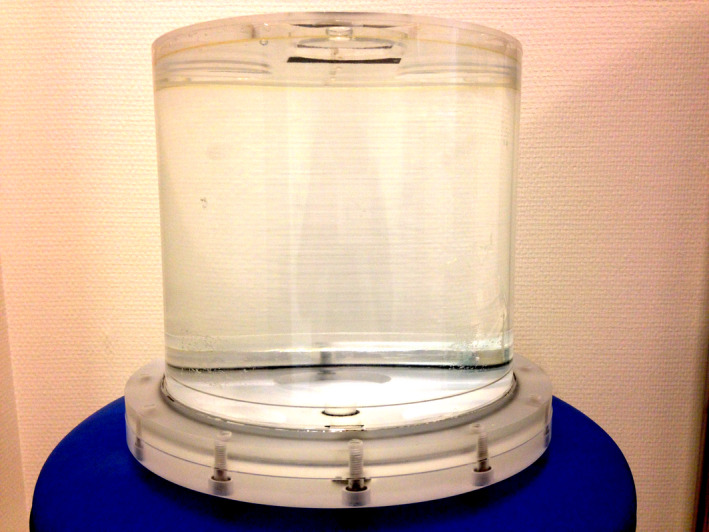
Cylindrical water tank phantom. Diameter: 20 cm; length: 25 cm. [Color figure can be viewed at wileyonlinelibrary.com]

Table 1.

Acquisition and reconstruction parameters

Parameter		Value
Acquisition	Pitch	1.375
	Rotation time (s)	1
	Tube voltage (kVp)	120
	Tube current (mA)	130	260
	CTDIvol (mGy)	7.5	15
	Collimation width (mm)	40
Reconstruction	Matrix size (pixel)	512 × 512
	Reconstruction algorithm	Filtered backprojection
	Kernel	Soft tissue
	Slice interval (mm)	2.5
	Slice thickness (mm)	2.5
	Field of view (mm)	300
	Pixel size (mm)	0.59

2.A.2. Image samples and signal

For simplicity, and because it was the first such exercise, we considered 2D image slices from CT acquisition. All image samples used were non‐overlapping squared regions of interest (ROI) of 200 × 200 pixels cropped from the original CT scans using only one slice every three slices to minimize any axial noise correlation. The investigated task was a binary classification in which the signal was present with 50 % prevalence. Signal present images were generated by inserting 6, 8, and 10 mm low contrast disk‐shaped signal mimicking hypodense focal liver lesion at the center of the image (location‐known‐exactly) with an alpha blending technique.²⁷ Figure 2 shows ROIs for 6, 8, and 10 mm signal sizes. The signal radial profile was fitted to real liver lesion profile using a contrast‐profile equation²⁸ and checked for its realism by an experienced radiologist. To ensure a non‐trivial task with human observers, the signal intensity was set to reach 90% to 95% of the correct answer in a pre‐study two‐alternative forced‐choice experiment (2‐AFC) with a 10 mm signal size involving three human observers. The same signal intensity was used for the two smaller signals.

Figure 2.

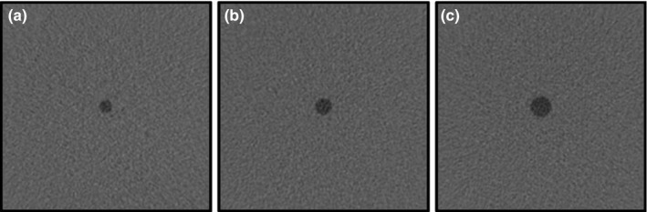
200 × 200 pixel size ROIs for (a) 6 mm, (b) 8 mm and (c) 10 mm signal size. These images were obtained by increasing signal contrast for visualization purposes.

2.A.3. Image dataset for observer study

We generated two Datasets. Dataset1 was intended to compare implementation of CHO model observer when the ground truth is available and Dataset2 was intended to assess model observers when the presence or absence of the signal in the image sample is unknown. Dataset1 contained images explicitly labeled in terms of presence or absence of the signal and corresponded to the 15 mGy dose level scans. Three image subsets were provided (1 for each signal size) and contained both 200 signal present and 200 signal‐absent samples. Dataset1 was provided in two versions: one without location cues for a model observer computation and another with location cues for human observer psychophysical experiments. Dataset2 was composed of 400 images obtained at half the dose of Dataset1 (CTDI_vol = 7.5 mGy) to provide a different dose condition with an 8 mm signal with a prevalence of 50%. The sequence of signal present and signal‐absent images was randomly defined and was different for each participating laboratory. The ground truth was kept unknown to each participant (including the co‐ordinating laboratory).

2.B. Task descriptions

All participating laboratories were asked to perform three tasks. The first two tasks were mandatory and consisted of computing the performance of a defined model observer. The other task was optional and consisted of estimating the performance of the human observer with a psychophysical experiment.

2.B.1. Performance computation with a defined model observer and Dataset1

Participants were asked to compute the performance of a defined model observer with Dataset1. We chose the CHO,^{5, 6, 7, 8} which is defined by a template derived from optimal weighting of a limited set of channel outputs. To get the template, each image is preprocessed by a set of J channels which reduces image dimension to the number of channels. Channel outputs are weighted to maximize detection performance using the dot product between the inverse of the covariance matrix and an estimation of the mean difference signal in the channel space. The decision variable from an image sample is derived from the dot product between the CHO template and the image sample vector in the channel space.

The D‐DOG channels in this exercise were those proposed by Abbey and Barrett,²⁹ which have the advantage to be precisely defined, sparse and mimic human observer.³⁰ DDOG radial spatial frequency profile functions are defined by

$$C_j(\rho )=exp\left(-\frac{1}{2}{\left(\frac{\rho }{Q{\sigma }_j}\right)}^2\right)-exp\left(-\frac{1}{2}{\left(\frac{\rho }{{\sigma }_j}\right)}^2\right)$$

where ${\sigma }_j={\sigma }_0{\alpha }^j$ is the channel standard deviation of the jth channel, and ${\sigma }_0$is the initial standard deviation. We used $j=10$ channels, ${\sigma }_0=0.005$ pixels⁻¹, $\alpha =1.4$, $Q=1.66$.

Different computations of CHO concern how the image samples are used or processed to derive the CHO features (e.g., template and mean signal, and decision variable distributions). The CHO computation methodology contains the following features: training and testing strategy, number of sample pairs in training and testing sets, ROI size, estimation of the covariance matrix with signal‐present and/or signal‐absent image samples, mean signal estimation, computation domain for image processing (space or frequency). The participants were free to use the image dataset as they wanted. The implementation details of the laboratories are documented in the Results section.

The participants were asked to estimate the detectability index d′, which is the distance between signal present and signal‐absent of decision variables distribution in standard deviation units; according to the definition given by Barrett and Myers.⁴ They were also asked to provide their uncertainty as being one standard‐deviation of their estimated probability density function of d′. In metrology, this uncertainty is called “standard uncertainty”.³¹ For a Gaussian distribution, this corresponds to a confidence level of 68% that the true value is within the interval. No instructions regarding the number of image samples to be used in the training and testing subsets of Dataset1 were given.

2.B.2. Performance of the same model observer and Dataset2

In the second mandatory task, participants were asked to compute test statistics using the same model observer as in the first task, but for Dataset2. The participants had the possibility to train the model observer using images from Dataset1, as the co‐ordinating laboratory did not provide additional images. As ground truth was unknown to them, participants reported the model's responses to each individual image. The detectability was computed by the co‐ordinating laboratory using the same definition as in 2.B.1.

2.B.3. Human observer with Dataset1

A voluntary exercise provided was to run human observer experiments with Dataset1. Participants could select the method to carry out the human study, and templates of the targets were provided together with the images for this task. They were asked to estimate d′ and its standard uncertainty u(d′) for the three signal sizes. For those who ran the experiments with more than one human observer, individual and pooled results were expected.

2.C. Study design

Each of the 13 participating laboratories was randomly assigned a participant number from 1 to 13. To guarantee some degree of confidentiality, each laboratory only knew its own number. The study packages were distributed through a secure server and participating laboratories could download them when they wanted. The study package contained Dataset1 and Dataset2, a description of the tasks, the study's milestones and a form to collect the raw results. The form content is described in Table 2. The complete form is available in the appendix.

Table 2.

Content of the results form to be filled by every participant

Section	Content
1. CHO D‐DOG with Dataset1	Quantitative estimation of detectability d′ and its uncertainty u(d′) for 6, 8 and 10 mm
	Qualitative description of model observer computation and uncertainty estimation method
	Covariance matrix for 6, 8 and 10 mm
2. CHO D‐DOG with Dataset2	Responses to Dataset2 image samples
3. Human observer with Dataset1 (optional)	Quantitative estimation of detectability d′ and its uncertainty u(d′) for 6, 8 and 10 mm
	Qualitative description of psychophysical experiment (material and settings)

Each laboratory had 2 months to return the results form. One month later, the results were distributed with each participant recognizable by its number. Each laboratory had the possibility to modify their results with justification within 1 month. We allowed this because model observer calculations are not yet a routine and still error prone. Moreover, as it was the first time that such an exercise was proposed, we needed to build trust to embark as many laboratories as possible into this study. Modified results are reported in Section Results. Results in the corresponding Figures and justifications are detailed in a dedicated paragraph in the Discussion section.

3. Results

Data from returned forms were analyzed and organized into two main sections: observer performances and computational methods. Table 3 shows the participation in the study respective to the tasks.

Table 3.

Summary of the participation in the three tasks

Participant number	Participation in the study
	CHO DDOG with Dataset1	CHO DDOG with Dataset2	Human observer with Dataset1	Number of human observers
1	Yes	Yes	Yes	4
2	Yes	Yes	Yes	10
3	Yes	Yes	‐	‐
4	Yes	Yes	‐	‐
5	Yes	Yes	Yes	1
6	Yes	Yes	‐	‐
7	Yes	Yes	‐	‐
8	Yes	Yes	‐	‐
9	Yes	Yes	Yes	3
10	Yes	Yes	‐	‐
11	Yes	Yes	‐	‐
12	Yes	Yes	Yes	1
13	Yes	Yes	Yes	3
Total	13	13	6	22

3.A. Quantitative results: Observer performances

3.A.1. Performance computation with a defined model observer and Dataset1

Detectability indexes computed by each laboratory for 6, 8, and 10 mm signal size are presented in Figure 3. Because the actual true detectability is not known, due to the use of actual CT data with an unknown underlying probability distribution, we chose the reference as being the median of all reported estimations. As expected d′ increased with signal size for all participants. The detectability index was very consistent for 6 mm and showed a somewhat higher variability for 8 and 10 mm for all participants with respectively less than 5%, 16%, and 18% variation between labs.

Figure 3.

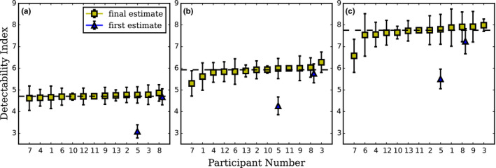
Detectability indexes for CHO D‐DOG with Dataset1 computed by each participant laboratories for (a) 6 mm, (b) 8 mm and (c) 10 mm signal size in increasing order. The dotted line represents the median value for final estimation of d′. For laboratories that corrected their estimation, the first estimation of d′ is plotted as a triangle marker. Error bars represent the 95% confidence interval for the mean d′. For the laboratories that provided standard uncertainties, the values were multiplied by a coverage factor k = 2 and are drawn as plus/minus this new value. [Color figure can be viewed at wileyonlinelibrary.com]

Figure 4 presents the uncertainty estimation of d′ computed by each participant for 6, 8, and 10 mm signal size, separately and in increasing order. They are presented as 95% confidence intervals with mention to the estimation method: resampling,³² exact 95% interval³³ and repartitioning. For the laboratories who reported a standard uncertainty, we implicitly assumed a Gaussian distribution and expanded their value by a coverage factor k = 2 to estimate a 95 % confidence interval (with k = 2 instead of the more precise value of 1.96, we followed the habit of the national metrological institutes, because the “uncertainty on the uncertainty” is much larger than the difference between 1.96 and 2). We observed one order of magnitude between the lowest and the largest uncertainty estimation.

Figure 4.

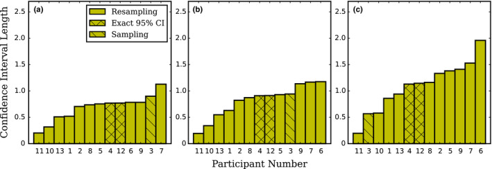
CHO D‐DOG with Dataset1 95% confidence interval length of the mean d′ computed by each participant laboratory for (a) 6 mm, (b) 8 mm and (c) 10 mm signal size in increasing order. For the laboratories that provided 1 standard‐deviation uncertainty, the values have been adjusted as described in the text. [Color figure can be viewed at wileyonlinelibrary.com]

The effect of the number of images, N, used to train CHO D‐DOG with Dataset1 on d′ for independent and resubstitution (the use of the same data for training and testing the CHO) sampling methods, was calculated by one of the participating laboratories, and is presented in Figure 5. The plot uses 1/N scale as d′‐versus‐1/N can be approached by a linear relationship and d′ for infinite sample size can be estimated by the intercept of a linear regression of d′‐versus‐1/N.³⁴ Estimation of d′ uncertainty decreased with increasing numbers of training images for both sampling methods. As expected, for resubstitution sampling, d′ decreases with increasing numbers of training images. For testing with independent samples, d′ increases with increasing numbers of training images. The two sampling methods converge and give approximately the same estimation of d′ from roughly 200 training images.

Figure 5.

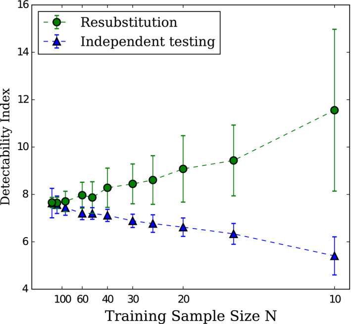
Effect of the number of samples N used to train the CHO on d′ for independent and resubstitution sampling methods with 10 mm signal size. Error bars represent the exact 95% interval as defined by Wunderlich et al.³³ The dotted lines are present to facilitate the reading of the graph. Courtesy of F. Samuelson and R. Zeng from FDA/CDRH. [Color figure can be viewed at wileyonlinelibrary.com]

3.A.2. Performance of the same model observer and Dataset2

Detectability indexes of the CHO D‐DOG computed on Dataset2 are presented in Figure 6. As expected, due to the lower dose of Dataset2, d′ median is lower than the one obtained with Dataset1. They also show a larger variability than Dataset1 with less than a 21% in variation between labs.

Figure 6.

CHO D‐DOG with Dataset2 d′ for 8 mm signal size in increasing order. The detectability index was computed by the exercise co‐ordinator from decision variable responses provided by each participant laboratory using the ground truth of the respecting Dataset. The detectability index was estimated as the distance between the mean signal present and absent distribution in sigma units. The dotted line represents the median value. Uncertainty estimates were computed by the co‐ordinator by bootstrapping the test cases from the decision variable responses provided by each participant with 1000 iterations. Errors bars represent two standard deviations from the bootstrapped d′ distribution. [Color figure can be viewed at wileyonlinelibrary.com]

3.A.3. Human observer with Dataset1

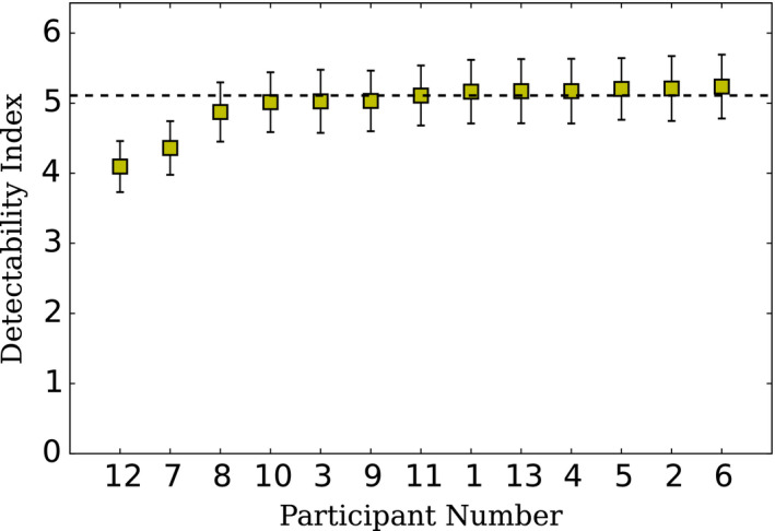
Human data provided by the participating laboratories with Dataset1 are presented in Figure 7. They show a much larger variability than the fixed D‐DOG estimation. For example, for the 10 mm signal size, there is a factor of 1.2 between minimum and maximum estimation of d′ for participating laboratories for CHO D‐DOG with Dataset1 and there is a factor of 2.5 for human observers with the same images.

Figure 7.

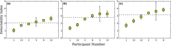
Detectability indexes for human observers with Dataset1 for participating laboratories for (a) 6 mm, (b) 8 mm, and (c) 10 mm signal size. The dotted line represents the median value. To derive d′ and u(d′) from MAFC, the hit/miss values were bootstrapped. Averaged PC was converted to d′ and errors bars represent u(d′) as 2 standard deviations from the bootstrapped distribution. [Color figure can be viewed at wileyonlinelibrary.com]

3.B. Qualitative results: comparison of the computational methods

The computational methods for CHO D‐DOG with Dataset1 are summarized in Table 4. Train‐test strategy and size of training and testing sets show how participants used image samples to estimate d′ from model observer decision variables. Eight participants chose resubstitution using the same set for training and testing. Among them, two participants (4 and 12) used an alternate resubstitution method with bias correction for the estimation of d′.³³ Four participants employed hold‐out using independent sets for training and testing. One participant split the testing set into eight independent samples and averaged d′ from all samples. All participants who applied the resubstitution method used a training size of 200 image pairs, and 100 image pairs were used for the hold‐out training and testing strategy, and one participant used the leave one out strategy. The testing size was 200 image pairs for resubstitution and 100 image pairs for hold‐out strategy.

Table 4.

CHO computation methodologies summary. The following features were identical for all participants and are not reported in the following table. ROI size = 200 × 200, mean signal estimation has been made “from samples” and the computational domain is the “image domain” rather than the “Fourier domain”

Participant	Train/test strategy	Sample pairs		d′ estimation 1: distance between signal present and signal‐absent distribution 2: signal‐to‐noise ratio	u (d′) estimation method	Source of variance 1: new training images 2: new test images 3: new train and test images	Number of resampling iterations	Covariance matrix estimation: signal absent & signal present 2: signal absent
		Training	Testing
1	Hold‐out	100	100	1	Bootstrap	2	1000	1
2	Resubstitution	200	200	1	Bootstrap	3	1000	1
3	Resubstitution	200	25	1	Repartition	2	‐	1
4	Resubstitution	200	200	2	Exact 95% CI	3	‐	1
5	Resubstitution	200	200	2	Bootstrap	3	1000	1
6	Other	200	200	1	Bootstrap	3	100	1
7	Hold‐out	100	100	1	Bootstrap	3	2000	1
8	Resubstitution	200	200	2	Bootstrap	3	1000	1
9	Resubstitution	200	200	1	Bootstrap	3	10,000	1
10	Hold‐out	100	100	1	Bootstrap	1	100	2
11	Hold‐out	199	1	1	Jack‐knife	3	200	1
12	Resubstitution	200	200	2	Exact 95% CI	3	‐	1
13	Resubstitution	200	200	1	Bootstrap	2	100	2

Most of the laboratories used resampling techniques for the estimation of u(d′), the uncertainty of d′. Resampling methods were bootstrap¹³ for nine participants and jack‐knife¹⁷ for one participant. The main differences between resampling techniques were if the training samples were fixed or variable. One participant split the testing set into eight independent parts and derived the standard deviation of d′ from all parts as an estimation of u(d′). Two participants used an exact formulation of the 95 % confidence interval³³ based on a method for the interval estimation of the Mahalanobis distance.³⁵

The estimation of d′ was systematically computed as the distance between the mean of signal present and signal‐absent decision variables distributions in the standard deviation unit as defined in Section 2.B.1, except for participant five who used a close form for the estimation of d′.⁴ For participants who used sampling or resampling techniques, d′ was the average d′ across all samples.

The estimation of the models' template components, such as the covariance matrix and mean signal, were systematically obtained from image samples. Figure 8 presents covariance matrices estimated by each participant for the 8 mm signal size. Every covariance matrices presents similar patterns, except for participants 7 and 11. The general pattern corresponds to high variance with high frequency channels that tend to decrease with lower frequency channels. For participant 7, the covariance matrix pattern was flatter than for the other participant and no scaling factor was found to explain the differences. For participant 11, the differences are explained as they did normalization of the channels so that sum of each one is one. All participants trained their observer on signal‐absent and signal‐present images together to estimate the channel covariance matrix, except for participants 10 and 13 who used signal‐absent images only. All participants computed the difference between the mean signal‐present and mean signal‐absent ensemble image sets as seen through the channels to estimate the mean signal.

Figure 8.

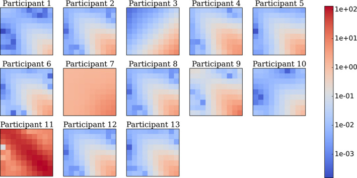
Covariance matrices K in channels space estimated by each participant for 8 mm signal size. In this representation, the top left pixel is the variance associated to the output of the lowest frequency channel and the bottom right pixel corresponds to the output of the highest frequency channel. All the other pixels describe the inter‐class covariance. As the exercise used 10 channels D‐DOG, K is a 10‐by‐10 matrix with the following array format: $K=\left[\begin{array}{ccc}{K}_{1,1}& \cdots & K_{1,10}\\ ⋮& \ddots & ⋮\\ K_{10,1}& \cdots & K_{10,10}\end{array}\right].$ [Color figure can be viewed at wileyonlinelibrary.com]

For all participants, ROI size was always the original size (200 × 200). All participants computed templates in the image domain. None used Fourier domain estimates.

The information concerning the psychophysical experiments performed with Dataset1 is summarized in Table 5. Six laboratories provided human data resulting to a total of 22 observers. Among them, seven were naive and 15 were experienced. There were no radiologists or otherwise clinically trained readers. All observers were trained before testing. All laboratories performed MAFC experiments with M = 2 alternatives for five participants and M = 4 alternatives for one participant. The metric derived from MAFC was the percent of correct (PC) answers for a given number of trials. For MAFC experiments involving more than one observer, the pool of observer outcomes was the averaged pc and the uncertainty was estimated by bootstrapping the pooled individual scores. No participant used multiple‐reader multiple‐case (MRMC) methods.

Table 5.

Psychophysical experiment design and derivation of human observer performance

Participant	Observers				Training	Type of experiment	Basic metric	Pool of observer outcomes	Estimation of uncertainty	Number of resampling iterations
	Total	Naive	Experienced	Radiologist
1	4	2	2	‐	Yes	2AFC	Percent correct	Average	Bootstrap	1000
2	10	5	5	‐	Yes	4AFC	Percent correct	Average	Bootstrap	100
5	1	‐	1	‐	Yes	2AFC	Percent correct	N/A	‐	‐
9	3	‐	3	‐	Yes	2AFC	Percent correct	Average	Bootstrap	10,000
12	1	‐	1	‐	Yes	2AFC	Percent correct	N/A	Bootstrap	1000
13	3	‐	3	‐	Yes	2AFC	Percent correct	Average	Bootstrap	1000

The material used to perform the psychophysical experiment is summarized in Table 6. Except for one laboratory who did not provide a value, the viewing illumination was low for each laboratory and varied from “dark” to 20 lux. The viewing distance was approximately 50 cm for all observers. Diagnostic and TFT monitors from various manufacturers were used with pixel size ranging from 0.20 to 0.60 mm. Minimum luminance ranged from 0 to 0.465 cd/m² and maximum luminance ranged from 405.7 to 1000 cd/m². All participants used diagnostic monitor except for participant 5.

Table 6.

Psychophysical experiment material specifications

Participant	Viewing illumination (lux)	Viewing distance (cm)	Type of monitor	Pixel size (mm)	Max. luminance (cd/m2)	Min. luminance (cd/m2)
	(lux)	(cm)		(mm)	(cd/m2)	(cd/m2)
1	10	50	NDS Dome E3	0.21	1000	0
2	N/A	40–50	BARCO 3MP LED	0.22	800	0
5	20	50	Standard TFT	N/A	N/A	N/A
9	<10	50	BARCO MDNC‐3121	0.21	405.7	0.465
12	Dark room	50	BARCO MD1119	0.60	162.9	0.01
13	Dark room	50	EIZO RADIFORCE	0.27	N/A	N/A

4. Discussion

This section is divided into different items that are each related with the major findings of the study.

4.A. Good coherence of model observer performance across participant laboratories

The main result of this study is that the performance of the CHO D‐DOG is reproducible across different laboratories for the three tested signal sizes (Figure 3). This outcome was expected as the model used for this exercise was precisely defined. The only degrees of freedom left to the laboratories were essentially how images were used to derive the model's features like the mean signal template and the covariance matrix, as well as how the model was trained and tested. With 200 signal‐present and 200 signal‐absent images, these aspects only had a minor effect on d′ as seen on Figure 5.

Concerning the derivation of the models' template components, mean signal estimation was identical among the participants, however, some differences in covariance matrices estimation were identified (Figure 8). Interestingly, the differences observed for participant 7 are consistent with their underestimation of d′ compared with other participants. For participant 11, the differences are explained because the approach used machine learning which then minimized the generalization error in predicting individual human observer scores on Dataset1.³⁶ While providing a different covariance matrix estimation, participant 11's d′ estimation was similar with other participants. Also, two participants (10 and 13) estimated the covariance matrix with the signal‐absent images only and did not obtain substantially different results than those who used both image classes. This result is consistent with previous results that suggest that both approaches are equivalent if the background is not affected by the signal like for the low contrast detection task as evaluated in this study.⁴

At first sight, it might be surprising that all participants produced such a coherent estimation of d′ since some of them used the resubstitution method for training and testing the models, and others used the hold‐out method. As shown in Figure 5, this may be due to the relative large number of available images. Two‐hundred images of each class were sufficient to have a similar estimation of d′ whatever the training/testing method. With 50 images only, the two estimation methods would have been significantly different: the strategies using resubstitution are expected to over‐estimate the performance while the strategies using hold‐out would under‐estimate the performance. However, the exact confidence interval estimation approach attempts to correct for the resubstitution and hold methods limitation; the resubstitution and hold‐out methods are estimating the performance of the finitely trained model and the exact confidence interval estimates a confidence interval for the performance of the infinitely trained model. Moreover, it can be seen that d′ fluctuates more between participants at high performances (18%) than at low performances (5%). This might be explained by the fact that at a higher performance level, the model observer's responses distribution present a larger standard deviation and are more prone to outliers. Therefore, more variability in d′ estimation between participants is expected.

4.B. Large range of uncertainty for model observer performance across participant

Because of a finite image sample, d′ is prone to bias estimation and an accurate assessment of its variability is important for making inferences. One of the findings of this work is that there is no consensus on what variance to present and is a limitation leading to widely disparate results. Figure 4 shows that there is an order of magnitude in the uncertainty estimation of the CHO performance among the participants. This reflects the various estimation methods and sampling strategies used in this exercise. All participants, except one, used resampling techniques like bootstrap or jackknife to generate multiple sets and derived the standard uncertainty as an estimation of the measurement uncertainty. However, large fluctuations are present in this group. Among them, some used fixed training sets and variable testing sets while others used both variable training and testing sets. Two participants (4 and 12) used a method described in Wunderlich et al.³³ and estimated the “exact 95 % confidence interval”, which led to consistent estimations between them. Participant 12 implemented the method while participant 4 used IQmodelo, a publicly available software package,³⁷ to estimate d′ uncertainty. The advantage of the exact 95 % confidence interval method resides in the unbiased direct estimation of d′ using the entire dataset even when the number of image samples is low.

4.C. More variations in model performances when the testing set is different than the training set

Our results suggest that this particular CHO‐DDOG implementation continues to be coherent when the testing set is different than the training set. As shown in Figure 6, testing the model on images with an unknown ground truth and a dose level 50 % lower than the training set still produces performances that are compatible among the different laboratories.

4.D. Large discrepancy of human observer performances

Although all human observers were well‐trained and experienced, and that the task was relatively easy, the performance varied widely among the participants (Figure 7). This cannot be explained by the type of monitors or their pixel size as most of them were similar (Table 6). However, how the participants displayed the images surely had an effect. For instance, all participants reported to have displayed the 8‐bit images without changing the LUT while participant 9 optimized the window width and level using the image histogram to increase the apparent contrast. This probably explains why participant 9 had the highest value of d′ for all signal sizes. Another source of explanation could be that human performances obtained by an MAFC experiment is the proportion correct (PC), which is then transformed into d′ by assuming Gaussian‐distributed internal responses. This operation stretches small differences in PC into larger differences in terms of d′. For example, for the 10 mm signal size, the estimated d′ ranged between 1.7 and 4.2. This corresponds to a variation between 89% and 100% in terms of PC. Finally, and more importantly, the fact that human observers are prone to inter‐ and intra‐variability has been an important motivation to use model instead of human observers.

4.E. A small number of participants chose to update their data

Participants were able to correct their outcomes after the initial release of the results to all the laboratories. Three participants took the opportunity to change their results. Participant 5 found an error in their implementation for Dataset1 with D‐DOG channels expressed in the Fourier domain instead of the image domain. They subsequently changed their model observer implementation in the image domain. With this change, the model observer performance was improved and is now closer to the other participants. Participant 8 resized the ROIs used for the calculation of CHO D‐DOG model observer with Dataset1 from 64 × 64 to the original size (200 × 200). This modification had a slight impact on d′ estimation as shown in Figure 3.

4.F. Limitations

This study was limited by the simplicity of the task investigated. A low‐contrast detection task in a uniform background is the simplest diagnostic task we can imagine, and future research could investigate different tasks and backgrounds from different imaging modalities. Another limitation is that the tested conditions were not very challenging since all three signal sizes reached a d′ larger than 4, which is virtually equivalent to area‐under‐the‐ROC‐curve equal to 1. It can be assumed that more challenging tasks (for example with a textured background, an unknown signal position, a smaller signal size or a sample with fewer images) would spread the estimation of d′ and its uncertainty. Another unchallenging aspect of this study was the relatively large number of image samples. With a smaller sample size, the estimation of the model template would be more difficult, and would probably induce more variation among the different laboratories. The many possible sources of variance and participant variance estimation methods could have been more precisely documented. A possible future investigation could collect and report what sources of variance are present in model observer methods and discuss the different variance estimates.

5. Conclusions

This comparison helped define the state of the art of the performance computation of model observers in a well‐defined situation. With thirteen participants, this reflects openness and trust within the medical imaging community.

The main result of this study is that the performance of a CHO with explicitly defined channels and a relatively large number of test images was consistently estimated by all participants. In contrast, the paper demonstrates that there is no agreement on estimating the variance of detectability in the training and testing setting.

The number of images is crucial for an accurate estimation of d′. In this study, the large number of available images did not lead to significant differences between the resubstitution and the hold‐out method. For less favorable conditions, exact 95% confidence interval method³³ has the advantage to include both reliable uncertainty estimation and bias correction.

This study also emphasizes the importance of the large variability in the human observer performance in psychophysical studies. This provides further motivation for the development of anthropomorphic model observers that can be used in place of human studies, and also suggests that we need further consensus on experimental settings for human‐observer studies.

Finally, this exercise should be considered a first step in evaluating the consistency of model observer computation for medical image quality assurance. A possible next exercise could involve clinical images with fewer samples. Meanwhile the images used for this exercise and the model and human scores are freely available for interested parties who did not take part and would like to compare their estimate of model observer detection performance with the present results.

Conflict of interest

The authors have no conflicts to disclose.

References

- 1. Brenner DJ, Hall EJ. Computed tomography — an increasing source of radiation exposure. N Engl J Med. 2007;357:2277–2284. [DOI] [PubMed] [Google Scholar]
- 2. McCollough CH, Chen GH, Kalender W, et al. Achieving Routine Submillisievert CT Scanning: report from the Summit on Management of Radiation Dose in CT. Radiology. 2012;264:567–580. [DOI] [PMC free article] [PubMed] [Google Scholar]
- 3. Parakh A, Kortesniemi M, Schindera ST. CT radiation dose management: a comprehensive optimization process for improving patient safety. Radiology. 2016;280:663–673. [DOI] [PubMed] [Google Scholar]
- 4. Barrett HH. Foundations of image science. Hoboken, NJ: Wiley‐Interscience; 2004. [Google Scholar]
- 5. Barrett HH, Yao J, Rolland JP, Myers KJ. Model observers for assessment of image quality. Proc Natl Acad Sci. 1993;90:9758–9765. [DOI] [PMC free article] [PubMed] [Google Scholar]
- 6. Gallas BD, Barrett HH. Validating the use of channels to estimate the ideal linear observer. J Opt Soc Am A. 2003;20:1725–1738. [DOI] [PubMed] [Google Scholar]
- 7. Yao J, Barrett HH. Predicting human performance by a channelized Hotelling observer model, in edited by D.C. Wilson and J.N. Wilson,1992, pp. 161–168.
- 8. Myers KJ, Barrett HH. Addition of a channel mechanism to the ideal‐observer model. J Opt Soc Am A. 1987;4:2447. [DOI] [PubMed] [Google Scholar]
- 9. Castella C, Ruschin M, Eckstein MP, et al. Mass detection in breast tomosynthesis and digital mammography: a model observer study, in edited by B. Sahiner and D.J. Manning, 2009, p. 72630O–72630O–10.
- 10. Young S, Bakic PR, Myers KJ, Jennings RJ, Park S. A virtual trial framework for quantifying the detectability of masses in breast tomosynthesis projection data. Med Phys. 2013;40:051914. [DOI] [PMC free article] [PubMed] [Google Scholar]
- 11. Srinivas Y, Wilson DL. Image quality evaluation of flat panel and image intensifier digital magnification in x‐ray fluoroscopy. Med Phys. 2002;29:1611–1621. [DOI] [PubMed] [Google Scholar]
- 12. Racine D, Ba AH, Ott JG, Bochud FO, Verdun FR. Objective assessment of low contrast detectability in computed tomography with Channelized Hotelling Observer. Phys Med. 2016;32:76–83. [DOI] [PubMed] [Google Scholar]
- 13. Yu L, Leng S, Chen L, Kofler JM, Carter RE, McCollough CH. Prediction of human observer performance in a 2‐alternative forced choice low‐contrast detection task using channelized Hotelling observer: impact of radiation dose and reconstruction algorithms. Med Phys. 2013;40:041908. [DOI] [PMC free article] [PubMed] [Google Scholar]
- 14. Hernandez‐Giron I, Calzado A, Geleijns J, Joemai RMS, Veldkamp WJH. Low contrast detectability performance of model observers based on CT phantom images: kVp influence. Phys Med. 2015;31:798–807. [DOI] [PubMed] [Google Scholar]
- 15. Brunner CC, Kyprianou IS. Material‐specific transfer function model and SNR in CT. Phys Med Biol. 2013;58:7447–7461. [DOI] [PubMed] [Google Scholar]
- 16. Brunner CC, Abboud SF, Hoeschen C, Kyprianou IS. Signal detection and location‐dependent noise in cone‐beam computed tomography using the spatial definition of the Hotelling SNR: spatial definition of the SNR in CBCT. Med Phys. 2012;39(6Part1):3214–3228. [DOI] [PubMed] [Google Scholar]
- 17. Brankov JG. Evaluation of the channelized Hotelling observer with an internal‐noise model in a train‐test paradigm for cardiac SPECT defect detection. Phys Med Biol. 2013;58:7159–7182. [DOI] [PMC free article] [PubMed] [Google Scholar]
- 18. Gifford HC. A visual‐search model observer for multislice‐multiview SPECT images. Med Phys. 2013;40:092505. [DOI] [PMC free article] [PubMed] [Google Scholar]
- 19. Gifford HC, King MA, Pretorius PH, Wells RG. A comparison of human and model observers in multislice LROC studies. IEEE Trans Med Imaging. 2005;24:160–169. [DOI] [PubMed] [Google Scholar]
- 20. Rupcich F, Badal A, Popescu LM, Kyprianou I, Gilat T. Schmidt, Reducing radiation dose to the female breast during CT coronary angiography: a simulation study comparing breast shielding, angular tube current modulation, reduced kV, and partial angle protocols using an unknown‐location signal‐detectability metric: reducing CT breast dose: a task‐based study. Med Phys. 2013;40:081921. [DOI] [PubMed] [Google Scholar]
- 21. Whitaker MK, Clarkson E, Barrett HH. Estimating random signal parameters from noisy images with nuisance parameters: linear and scanning‐linear methods. Opt Express. 2008;16:8150. [DOI] [PMC free article] [PubMed] [Google Scholar]
- 22. Tseng H‐W, Fan J, Kupinski MA. Design of a practical model‐observer‐based image quality assessment method for x‐ray computed tomography imaging systems. J Med Imaging. 2016;3:035503. [DOI] [PMC free article] [PubMed] [Google Scholar]
- 23. Goffi M, Veldkamp WJH, Engen RE, Bouwman RW. Evaluation of six channelized Hotelling observers in combination with a contrast sensitivity function to predict human observer performance, in edited by C.R. Mello‐Thoms and M.A. Kupinski, 2015, p. 94160Z.
- 24. Bailat C, Buchillier T, Caffari Y, et al. Seven years of gamma‐ray spectrometry interlaboratory comparisons in Switzerland. Appl Radiat Isot. 2010;68:1256–1260. [DOI] [PubMed] [Google Scholar]
- 25. Kossert K, Thieme K. Comparison for quality assurance of 99mTc activity measurements with radionuclide calibrators. Appl Radiat Isot. 2007;65:866–871. [DOI] [PubMed] [Google Scholar]
- 26. Coultre RL, Bize J, Champendal M, et al. Exposure of the swiss population by radiodiagnostics: 2013 review. Radiat Prot Dosim. 2015;169:221–224. [DOI] [PMC free article] [PubMed] [Google Scholar]
- 27. Shin H, Blietz M, Frericks B, Baus S, Savellano D, Galanski M. Insertion of virtual pulmonary nodules in CT data of the chest: development of a software tool. Eur Radiol. 2006;16:2567–2574. [DOI] [PubMed] [Google Scholar]
- 28. Solomon J, Samei E. A generic framework to simulate realistic lung, liver and renal pathologies in CT imaging. Phys Med Biol. 2014;59:6637–6657. [DOI] [PubMed] [Google Scholar]
- 29. Abbey CK, Barrett HH. Human‐ and model‐observer performance in ramp‐spectrum noise: effects of regularization and object variability. J Opt Soc Am.A Opt Image Sci Vis. 2001;18:473–488. [DOI] [PMC free article] [PubMed] [Google Scholar]
- 30. He X, Park S. Model observers in medical imaging research. Theranostics. 2013;3:774–786. [DOI] [PMC free article] [PubMed] [Google Scholar]
- 31. BIPM I, IFCC I, ISO I, IUPAP O. Evaluation of measurement data — an introduction to the “Guide to the expression of uncertainty in measurement” and related documents, 2009.
- 32. Efron B. The Jackknife, the bootstrap and other resampling plans. Philadelphia, PA: Society for Industrial and Applied Mathematics, 1982. [Google Scholar]
- 33. Wunderlich A, Noo F, Gallas B, Heilbrun M. Exact confidence intervals for channelized hotelling observer performance in image quality studies. IEEE Trans Med Imaging. 2014;34:453–464. [DOI] [PMC free article] [PubMed] [Google Scholar]
- 34. Chan H‐P, Sahiner B, Wagner RF, Petrick N. Classifier design for computer‐aided diagnosis: effects of finite sample size on the mean performance of classical and neural network classifiers. Med Phys. 1999;26:2654–2668. [DOI] [PubMed] [Google Scholar]
- 35. Reiser B. Confidence intervals for the mahalanobis distance. Commun Stat – Simul Comput. 2001;30:37–45. [Google Scholar]
- 36. Massanes F, Brankov JG. Human template estimation using a Gaussian processes algorithm. edited by C.R. Mello‐Thoms and M.A. Kupinski (2014), p. 90370Y.
- 37. IQmodelo . Statistical software for task‐based image quality assessment with model (or Human) observers. http://didsr.github.io/IQmodelo/