

Abstract
Deep neural networks (DNNs) represent the mainstream methodology for supervised speech enhancement, primarily due to their capability to model complex functions using hierarchical representations. However, a recent study revealed that DNNs trained on a single corpus fail to generalize to untrained corpora, especially in low signal-to-noise ratio (SNR) conditions. Developing a noise, speaker, and corpus independent speech enhancement algorithm is essential for real-world applications. In this study, we propose a self-attending recurrent neural network (SARNN) for time-domain speech enhancement to improve cross-corpus generalization. SARNN comprises of recurrent neural networks (RNNs) augmented with self-attention blocks and feedforward blocks. We evaluate SARNN on different corpora with nonstationary noises in low SNR conditions. Experimental results demonstrate that SARNN substantially outperforms competitive approaches to time-domain speech enhancement, such as RNNs and dual-path SARNNs. Additionally, we report an important finding that the two popular approaches to speech enhancement: complex spectral mapping and time-domain enhancement, obtain similar results for RNN and SARNN with large-scale training. We also provide a challenging subset of the test set used in this study for evaluating future algorithms and facilitating direct comparisons.
Keywords: Speech enhancement, cross-corpus generalization, self-attention, recurrent neural network, time-domain enhancement
I. Introduction
Background noise is unavoidable in the real world. It reduces the intelligibility and quality of a speech signal for human listeners. Additionally, it can severely degrade the performance of speech-based applications, such as automatic speech recognition, speaker identification, and hearing aids. Speech enhancement aims at removing or attenuating background noise from a noisy speech signal. It is used as a preprocessor in speech-based applications to improve their performance in noisy environments. Monaural speech enhancement, which is the task of speech enhancement from single microphone recordings, is considered an extremely challenging problem, especially in the presence of nonstationary noises in low signal-to-noise ratio (SNR) conditions. This study focuses on monaural speech enhancement in the time domain.
Traditional approaches to monaural speech enhancement include spectral subtraction, Wiener filtering and statistical model-based methods [1]. In recent years, supervised approaches to speech enhancement using deep neural networks (DNNs) have become the mainstream methodology for speech enhancement [2], primarily due to their capability to learn complex relations from supervised data by using hierarchical representations.
Speech enhancement mainly uses time-frequency representations, such as short-time Fourier transform (STFT), for extracting input features and training targets. Training targets play an important role in DNN performance and can be either masking based or mapping based. Masking based targets, such as ideal ratio mask [3] and phase sensitive mask [4], are based on time-frequency (T-F) relations between the noisy and the clean speech, whereas mapping based targets, such as spectral magnitude and log-spectral magnitude are based on clean speech [5], [6]. DNN is trained in a supervised way to estimate training targets from input features. During evaluation, the enhanced waveform is obtained by reconstructing a signal from the estimated training target.
Most of the popular approaches to speech enhancement aim at enhancing only the spectral magnitude and use unaltered noisy phase for time-domain reconstruction [5], [6], [7], [8], [9], [10], [11], [12], [13]. This is primarily due to a belief that spectral phase is unimportant for speech enhancement, and it exhibits no T-F structure amenable to supervised learning [14]. However, a relatively recent study has demonstrated that phase can play an important role in the quality of enhanced speech, especially in low SNR conditions [15]. As a result, researchers have started exploring ways to enhance both the spectral magnitude and the spectral phase. The first study in this regard was done by Williamson et al. [14], where the Cartesian representation of STFT in terms of real and imaginary parts was used instead of the widely used polar representation to propose complex ratio masking due to the T-F structure in the Cartesian representation. Complex ratio masking was further utilized in many studies, such as [16], [17], [18]. Complex spectral mapping, a related approach for jointly enhancing the magnitude and the phase, aims at directly predicting the real and the imaginary part of the clean spectrogram from the noisy spectrogram [19], [20], [21], [22].
On the other hand, time-domain speech enhancement aims at directly predicting the clean speech samples from the noisy speech samples, and in the process, magnitude and phase are jointly enhanced [23], [24], [25], [26], [27], [28], [29]. It does not require computations associated with the conversion of a signal to and from the frequency domain, and feature extraction becomes an implicit part of supervised learning.
The study in [23] proposed a fully convolutional neural network (CNN) for time-domain speech enhancement. Time-domain speech enhancement was further improved by using better processing blocks, such as dilated convolutions [25], [26], [29], dense connections [30], self-attention [31], [32], and dual-path recurrent neural networks (RNNs) [33], [34].
Additionally, time-domain speech enhancement has benefited from better optimization methods, such as adversarial training [24] and better loss functions, such as a loss incorporating the objective metric of short-time objective intelligibility (STOI) [35], [27] or spectral magnitudes [36], [28]. The STOI-based loss in [27] was able to improve STOI but was found to be suboptimal for objective quality metric, perceptual evaluation of speech quality (PESQ) [24], and segmental SNR. The spectral magnitude based loss [36], [28], on the other hand, was able to improve both STOI and PESQ but was suboptimal for scale-invariant SNR. In [32], the spectral magnitude based loss was found to exhibit an artifact in the enhanced audio, which was subsequently removed by using an improved loss called phase constrained magnitude (PCM). The PCM loss not only removed the artifact but also obtained consistent improvement for different metrics, such as STOI, PESQ, and SNR.
Recently, it has been revealed that DNNs trained for speech enhancement do not generalize to untrained corpora, especially in low SNR conditions [37]. Even time-domain enhancement networks, such as auto-encoder convolutional neural network (AECNN) [28] and temporal convolutional neural network (TCNN) [29], that exhibit strong performance for untrained speakers from the training corpus, fail to generalize to speakers from untrained corpora. It is revealed that the corpus channel unwillingly acquired due to recording conditions is one of the main culprits for performance degradation from trained to untrained corpora. Several techniques were proposed to improve cross-corpus generalization, such as channel normalization, a better training corpus, and a smaller frame shift [37]. The proposed techniques obtain significant improvements on untrained corpora for an IRM-based long short-term memory (LSTM) recurrent neural network (RNN). This work was further extended to complex spectral mapping with improved cross-corpus generalization [22]. An interesting finding in [22] is that a sophisticated architecture for complex spectral mapping, gated convolutional neural network (GCRN), which obtains impressive performance on trained corpora, fails to generalize to untrained corpora. Further, simple LSTM RNNs with a smaller frame shift are found to be very helpful for cross-corpus generalization.
Self-attention is a widely utilized mechanism for sequence-to-sequence tasks, such as machine translation [38], image generation [39] and ASR [40]. It was first introduced in [38], which obtained start-of-the-art performance for sequence-to-sequence tasks by using networks comprising self-attention blocks only. In self-attention, a given output in a sequence is computed using a subset of the input sequence that is helpful for the output prediction. In other words, an output is predicted by attending to a subset of the input for improving output prediction. Many recent studies [31], [41], [42], [43], [44], [34], [32], [45], [18] have employed self-attention for speech enhancement and reported significant improvements.
Nicolson et al. [44] developed a network similar to the encoder of the transformer network [38] for a priori SNR estimation. The estimated SNR was used with a minimum-mean square error (MMSE) log-spectral amplitude estimator for magnitude enhancement. In a subsequent study [45], a similar network was employed for predicting linear predictive coding (LPC) power spectra, which was utilized with an augmented Kalman filter for time-domain speech enhancement. Zhao et al. [41] used self-attention within a CNN for spectral mapping based magnitude enhancement for speech dereverberation.
Self-attention for complex ratio masking and complex spectral mapping has been studied for speech enhancement. A complex-valued transformer with Gaussian-weighted self-attention mechanism was proposed in [42]. A speaker-aware network using self-attention was investigated in [43], and a self-attention mechanism within a convolutional recurrent network was utilized in [18].
The first study to use self-attention for time-domain speech enhancement was reported in [31], which proposed a self-attention mechanism within a 1-dimensional UNet [46]. Pandey et al. proposed to use self-attention within layers of a dense UNet, which comprised dense blocks within encoder and decoder layers. A recent study [34] also investigated self-attention with a dual-path RNN for time-domain speech enhancement. However, we find that time-domain self-attending networks, such as the ones in [32] and [34], obtain subpar performance on untrained corpora.
In this work, we propose a self-attending RNN (SARNN) for time-domain speech enhancement to improve cross-corpus generalization. SARNN comprises RNN augmented with a self-attention block and a feedforward block. The proposed SARNN is motivated by observations such as RNNs with a smaller frame shift are helpful for cross-corpus generalization [37], [22], and self-attention is a general mechanism effective for speech enhancement [31], [41], [42], [43], [44], [34], [32], [45], [18]. We employ an efficient attention mechanism proposed specifically for RNN [47], which results in reduced memory consumption, faster training, and similar or better performance than the widely used attention mechanism in [38].
We find that self-attention mechanism in SARNN leads to substantial improvement on untrained corpora. Further, SARNN outperforms existing approaches to speech enhancement in terms of cross-corpus generalization. Additionally, we compare complex spectral mapping and time-domain enhancement for RNN and SARNN and find that complex spectral mapping and time-domain enhancement obtain statistically similar results when trained on a large corpus.
We find a subset of our test set to be particularly challenging for improving objective intelligibility and quality scores. To stimulate progress, we make this test set available online for evaluating future algorithms and facilitating direct comparisons.
The rest of the paper is organized as follows. Section II describes time-domain speech enhancement. Section III presents the details of SARNN building blocks and Section IV describes SARNN architecture for time-domain speech enhancement. Experimental settings are given in Section IV, and results and comparisons are presented in Section V. Concluding remarks are given in Section VI.
II. Time-domain speech enhancement
A noisy speech signal x is defined as the sum of a clean speech signal s and a noise signal n
| (1) |
, and M is the number of samples in the speech signal. A speech enhancement algorithm aims at obtaining a close estimate, ŝ, of s given x.
The goal of a time-domain speech enhancement algorithm is to compute ŝ directly from x instead of using a T-F representation of x. Time-domain speech enhancement using a DNN can be formulated as
| (2) |
where fθ denotes a function represented by a DNN parametrized by θ.
A. Frame-Level Processing
Generally, a speech enhancement algorithm is designed to process frames of a speech signal. Given a noisy signal x, it is first chunked into overlapping frames which is then processed at frame-level by a speech enhancement model. Let denote the matrix containing frames of signal x and the tth frame. xt is defined as
| (3) |
where T is the number of frames, L is the frame length, and J is the frame shift. T is given by , where ⌈ ⌉ denotes the ceiling function. x is padded with zeros if M is not divisible by J. Frame-level processing using a DNN can be defined as
| (4) |
where is computed using xt, T1 past frames, and T2 future frames.
B. Causal Speech Enhancement
A frame-level speech enhancement algorithm is considered causal if the estimation of a given frame is computed using noisy frames at time instances less than or equal to t. For causal speech enhancement Eq. (4) is modified as
| (5) |
where is computed using xt and T1 past frames.
Causality is a necessary requirement for real-time speech enhancement. Further, we observe that a causal algorithm exhibits greater degradation on untrained corpora compared to a corresponding non-causal algorithm. Therefore, we also develop and compare causal algorithms.
III. Self-attending Recurrent Neural Network
A block diagram of SARNN is given in Fig. 1. The building blocks of SARNN are layer normalization, RNN, self-attention block, and feedforward block. Next, we describe these building blocks one by one.
Fig. 1:
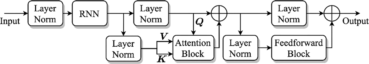
A diagram of SARNN. Layer Norm denotes a layer-normalization layer and ⨁ is an elementwise addition operator.
A. Layer Normalization
Layer normalization is a popular normalization technique used within DNNs to improve generalization and facilitate faster training [48]. It was proposed as an alternative to batch normalization [49], which is found to be sensitive to training batch size.
Let be a matrix and xt be its tth row. We use the layer normalization defined as
| (6) |
where and , respectively, are mean and variance of xt. Symbols γ and β are trainable parameters of the same size as xt, ⊙ denotes elementwise multiplication, and ∊ is a small positive constant used to avoid division by zero.
B. Recurrent Neural Network
We use LSTM RNN in SARNN. An illustrative diagram of an LSTM is shown in Fig. 2. Given an input vector sequence {x1, …, xt−1, xt, xt+1, …, xT}, the hidden state at time t, ht, is computed as
| (7) |
| (8) |
| (9) |
| (10) |
| (11) |
| (12) |
| (13) |
| (14) |
where xt, gt, and ct respectively represent input, block input, and memory (cell) state at time t. In additions it, ft, and ot are gates known as input gate, forget gate and output gate, respectively. W’s and b’s denote trainable weights and biases.
Fig. 2:

A diagram of an LSTM with three gates. Symbol ⊗ denotes elementwise multiplication.
C. Self-attention Block
A general attention mechanism is defined using three components: key , value , and query . First, correlation scores between pairs of rows from Q and K, {Qi, Kj}, where i, j ∈ {1, … , T}, are computed using the following equation.
| (15) |
where and denotes the transpose of K. The similarity scores in W are converted to probability values using the Softmax operation defined as
| (16) |
The final attention output is defined as the linear combination of the rows of V with weights in Softmax(W).
| (17) |
In self-attention, K,V, and Q are computed from the same sequence. One of the approaches to self-attention is to use three linear projections of a given input, , to obtain K,V, and Q, and then applying Eqs. (15)–(17) to obtain the attention output.
A block diagram of the attention block in SARNN is shown in Fig. 3. It comprises three trainable vectors and its inputs are . Let qt, vt, and kt denote the tth row in Q, V, and K respectively, and they are refined using gating mechanisms in the following equations.
| (18) |
| (19) |
| (20) |
where σ is sigmoidal nonlinearity, and Lin() is a linear layer. Note that σ(Lin(v)) ⊙ Tanh(Lin(v)) represents a constant vector computed from v. This operation is used during training only for better optimization of v. For evaluation, we use its value from the best model at training completion.
Fig. 3:

Attention block in SARNN. The inputs to the block are qt, kt, and vt and the output from the block is at.
The final output of the attention block is computed as
| (21) |
| (22) |
D. Feedforward Block
The feedforward block in SARNN is shown in Fig. 4. A given input of size N is projected to size 4N using a linear layer, which is followed by Gaussian error linear unit (GELU) [50] and a dropout layer [51]. Finally, the output of size 4N is split into four vectors of size N, which are added together to get the final output.
Fig. 4:

Feedforward block in SARNN.
With the building blocks described, we now present the processing flow of SARNN shown in Fig. 1. The input to SARNN is first normalized and then processed using an RNN. The output of the RNN is normalized using two parallel layer normalizations. The first stream is used as Q and the second stream is used as K and V for the following attention block. The output of the attention block is added to Q to form a residual connection. Again, the output is normalized using two parallel layer normalizations. The first stream is processed using a feedforward block and the second stream is added to the output of the feedforward block to form a residual connection.
IV. SARNN for Time-Domain Speech Enhancement
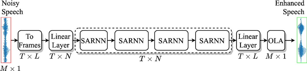
The proposed SARNN for time-domain speech enhancement is shown in Fig. 5. Given an input signal x with M samples, it is first chunked into overlapping frames with a frame size of L and frame shift of J to obtain T frames. Next, all the frames are projected to a representation of size N using a linear layer, which is then processed using four SARNNs. We use four-layered SARNN as a simple extension of the four-layered RNN for complex spectral mapping in [22]. A linear layer at the output projects the output of the last SARNN to size L. Finally, overlap-and-add (OLA) is used to obtain the enhanced waveform.
Fig. 5:
The proposed SARNN for time-domain speech enhancement.
A. Non-causal Speech Enhancement
For non-causal speech enhancement, we use BLSTM RNN inside SARNN. A BLSTM comprises two LSTMs; a forward and a backward LSTM. The forward LSTM operates over the sequence in the original order, whereas the backward LSTM operates over the sequence in the reverse order. Let and denote the sequence in the original and reverse order respectively. Then, we have
| (23) |
| (24) |
The hidden state at time t for a BLSTM is given as
| (25) |
where [a, b] denotes a concatenation of vectors a and b, and LSTMf and LSTMb represent the forward and the backward LSTM.
B. Causal Speech Enhancement
For causal speech enhancement, we use LSTM RNN and causal attention inside SARNN. Causal attention is implemented by applying a mask to W′ where entries above the main diagonal are set to negative infinity so that the contribution from future frames in Eq. (22) becomes zero. The causal attention is defines as
| (26) |
where
| (27) |
V. Experimental Settings
A. Datasets
We evaluate all the models in a speaker, noise, and corpus independent way. We use all utterances from the training set of LibriSpeech corpus [52] to generate training mixtures. It consists of around 280K speech utterances of more than 2000 speakers. LibriSpeech has been shown to be an effective corpus for cross-corpus generalization because it is recorded by many volunteers across the globe, and hence consists of utterances recorded in different acoustic conditions. Noisy training utterances are generated in an online fashion during training in the following way. For each sample in a given batch, we randomly sample a speech utterance, extract a random chunk of 4 seconds from it, and add a random chunk of noise to it at a random SNR from {−5, −4, −3, −2, −1, 0} dB. The sampled speech is used unaltered if its duration is smaller than 4 seconds. A set of 10000 non-speech sounds from a sound effect library (www.sound-ideas.com) are used as the training noises.
All the models are evaluated on three different corpora: WSJ-SI-84 (WSJ) [53], TIMIT [54], and IEEE [55], which are not used during training. We use utterances of one male speaker and one female speaker from IEEE to further categorize IEEE as IEEE Male and IEEE Female to show potential gender effects. The WSJ test set consists of 150 utterances of 6 different speakers. The TIMIT test set consists of 192 utterances in the core test set. IEEE Male and IEEE Female each consists of 144 randomly selected utterances. We generate noisy utterances using four different types of noises: babble, cafeteria, factory, and engine, none of which are used during training. Test utterances are generated at 6 different SNRs of −5, −2, 0, 2, and 5 dB. We find corpus fitting to be a severe issue for the difficult noises of babble and cafeteria, and at low SNRs of −5 dB and −2 dB. Therefore, for the sake of the brevity, we report results only for babble and cafeteria noises at SNRs of −5 dB and −2 dB. We observe similar performance trends for the other noises and SNR conditions. Note that our test set is the same as the one previously used in [37] and [22]. Babble and cafeteria noises are taken from an Auditec CD (available at http://www.auditec.com). Factory and engine noises are taken from the Noisex dataset [56]. We use WSJ test utterances mixed with babble noise at the SNR of −5 dB as the validation set.
We find our IEEE Male and IEEE Female test set to be relatively challenging in terms of improving the intelligibility and quality of unprocessed mixtures. In particular, IEEE utterances mixed with babble and cafeteria noises at SNRs of −5 dB and −2 dB are very difficult. Therefore, we provide online IEEE Male and IEEE Female utterances mixed with babble and cafeteria noises at SNRs of −5 dB and −2 dB as a useful test set for evaluating future algorithms and facilitating direct comparisons. It can be downloaded at https://web.cse.ohio-state.edu/~wang.77/pnl/corpus/Pandey/NoisyIEEE.html.
In addition we investigate the proposed model for speech quality improvement in relatively high SNR conditions. We train SARNN on the VCTK dataset [57] and compare it with a number of existing models evaluated on this task. The VCTK training set consists of utterances from 28 speakers mixed with different noises at SNRs of 0, 5, 10 and 15 dB. We exclude two speakers (p274 and p282) from the training set to create a validation set. The test set comprises utterances from two unseen speakers (not in the training set) mixed with different noises at 2.5, 7.5, 12.5, and 17.5 dB. We store training speech and noises separately and dynamically mix them during training using random SNRs from {0, 5, 10, 15} dB. The same SNR values are used as in the original training set. The dynamic mixing provides a measure of data augmentation, as similarly done in [58].
We also evaluate our model on real recordings. We utilize the blind test set from the second deep noise suppression (DNS) challenge [59], which consists of 650 real recordings and 50 synthetic mixtures. This test set is divided into five classes of English, non-English, tonal, singing, and emotional speech. To create a training set, we use speech and noises from the third DNS challenge [60]. We remove low quality utterances from all classes using appropriate thresholds on provided parameter T60_WB. We use room impulse responses (RIRs) with T60_WB between 0.3 and 0.9. The final training set consists of 347K speech utterances, 65K noises, and 47K RIRs. We generate training mixtures dynamically by convolving a speech signal with a random RIR and adding a random noise segment. We add room reverberation with a probability of 0.5. When using an RIR, the training target is set to be the clean speech convolved with the first 50 ms of the RIR. We sample a SNR value uniformly from either {−5, −4, …, −1, 0} dB or from {1, 2, …, 19, 20} dB with a probability of 0.5.
B. System Setup
All the utterances are resampled to 16 kHz, and leading and trailing silences are removed from training utterances. Each noisy mixture is normalized using root mean square (RMS) normalization and the corresponding clean utterance is scaled accordingly to maintain an SNR.
Parameter N is set to 1024, input frame size is set to 32 ms for causal system and 16 ms for non-causal system, and output frame size is set to 16 ms. For SARNN with BLSTM, N = 1024 results in a hidden state size of 512 in both forward and backward LSTM. A dropout rate of 5% is used in the feedforward block of SARNN. We use the utterance level MSE (mean squared error) loss in the time domain for training on Librispeech and the PCM (phase constrained magnitude) loss [32] for training on VCTK and DNS. The MSE loss is defined in the time domain as follows
| (28) |
The PCM loss is defined in the T-F domain that measures the distance between clean and estimated magnitude spectrum of both speech and noise. It is defined using the following set of equations.
| (29) |
| (30) |
| (31) |
where S and respectively denote STFTs of s and , T is the number of time frames, and F is the number of frequency bins.
The Adam optimizer [61] is used for training. A batch size of 32 utterances is used on Librispeech and DNS and that of 8 on VCTK. Models are trained for 100 epochs on Librispeech, 84 epochs on DNS, and 200 epochs on VCTK. A constant learning rate of 0.0002 is used for the first 33 (28 for DNS) epochs, after which it is exponentially decayed using a scale that results in a learning rate of 0.00002 in the final epoch. During training, we evaluate a given model on the validation set every two epochs, and the model parameters corresponding to the best SNR are chosen for evaluation.
We develop all the models in PyTorch [62] and exploit automatic mixed precision training to expedite training [63]. Two NVIDIA Volta V100 32GB GPUs are required to train SARNN with a batch size of 32 utterances. A given batch is equally distributed to two GPUs using PyTorch’s DataParallel module.
C. Baseline Models
We train five different models as the baselines for comparing corpus-independent models trained on Librispeech. First, we train a recently proposed deep complex convolutional recurrent network (DCCRN) [17], which respectively won the first and the second place in real-time and non-real-time track of the first DNS challenge [64]. DCCRN uses noisy complex spectrum as the input and the complex ideal ratio mask (cIRM) as the training target. Next, we train two RNN-based models; RNN-IRM [37] and RNN-TCS [22]. RNN-IRM uses log spectral magnitude as the input feature and the IRM as the training target. RNN-TCS uses noisy complex spectrum as the input feature and the target complex spectrum (TCS) as the training target. Finally, we train two recently proposed time-domain networks; dense convolutional network with self-attention (DCN) [32] and dual-path SARNN (DPSARNN) [34]. Even though DCN and DPSARNN obtain good enhancement in the time domain, they have not been trained and evaluated in a corpus-independent way.
The SARNN model trained on VCTK is compared with a number of existing methods that report performance on the same dataset (see Table III). The SARNN model trained on the DNS challenge dataset is compared with a baseline noise suppression network (NSNet) provided with the third DNS challenge [60].
TABLE III:
Comparing MSE loss and PCM loss at SNRs of −5 dB and 5 dB. a) Non-causal, b) causal.
| Test Corpus | WSJ | TIMIT | IEEE Male | IEEE Female | |||||||
|---|---|---|---|---|---|---|---|---|---|---|---|
|
| |||||||||||
| Test SNR | −5 dB | 5 dB | −5 dB | 5 dB | −5 dB | 5 dB | −5 dB | 5 dB | |||
|
| |||||||||||
| Babble | STOI (%) | Noisy | 58.6 | 81.2 | 54.0 | 77.1 | 55.0 | 79.4 | 55.5 | 80.3 | |
|
| |||||||||||
| (a) | MSE | 91.1 | 97.1 | 84.5 | 96.1 | 82.3 | 95.6 | 85.6 | 96.8 | ||
| PCM | 92.0 | 97.6 | 84.9 | 96.7 | 81.5 | 95.9 | 84.8 | 97.2 | |||
|
| |||||||||||
| (b) | MSE | 88.3 | 96.6 | 80.2 | 95.3 | 77.7 | 94.6 | 80.1 | 96.1 | ||
| PCM | 88.8 | 97.1 | 80.4 | 95.9 | 77.7 | 94.9 | 78.4 | 96.5 | |||
|
| |||||||||||
| PESQ | Noisy | 1.54 | 2.12 | 1.46 | 2.08 | 1.45 | 2.06 | 1.12 | 1.86 | ||
|
| |||||||||||
| (a) | MSE | 2.82 | 3.36 | 2.43 | 3.31 | 2.45 | 3.31 | 2.48 | 3.36 | ||
| PCM | 2.98 | 3.57 | 2.52 | 3.48 | 2.41 | 3.40 | 2.47 | 3.57 | |||
|
| |||||||||||
| (b) | MSE | 2.50 | 3.25 | 2.15 | 3.13 | 2.16 | 3.14 | 2.10 | 3.18 | ||
| PCM | 2.57 | 3.42 | 2.14 | 3.27 | 2.08 | 3.20 | 1.99 | 3.37 | |||
|
| |||||||||||
| SI-SNR | Noisy | −5.0 | 5.0 | −5.0 | 5.0 | −5.0 | 5.0 | −5.0 | 5.0 | ||
|
| |||||||||||
| (a) | MSE | 10.9 | 17.2 | 8.9 | 16.3 | 7.5 | 14.6 | 8.1 | 16.0 | ||
| PCM | 10.9 | 17.2 | 8.8 | 16.3 | 6.7 | 14.6 | 7.5 | 16.1 | |||
|
| |||||||||||
| (b) | MSE | 9.1 | 16.6 | 7.2 | 15.5 | 5.3 | 13.9 | 5.8 | 15.3 | ||
| PCM | 9.1 | 16.6 | 7.2 | 15.6 | 5.3 | 13.8 | 5.1 | 15.3 | |||
|
| |||||||||||
| Cafeteria | STOI (%) | Noisy | 57.4 | 81.2 | 53.1 | 76.2 | 54.8 | 77.0 | 55.1 | 78.4 | |
|
| |||||||||||
| (a) | MSE | 88.3 | 96.4 | 82.7 | 95.1 | 80.6 | 94.0 | 85.3 | 95.9 | ||
| PCM | 89.0 | 96.9 | 84.0 | 95.8 | 81.0 | 94.4 | 86.1 | 96.4 | |||
|
| |||||||||||
| (b) | MSE | 84.7 | 95.7 | 79.0 | 94.0 | 75.5 | 92.6 | 80.3 | 95.1 | ||
| PCM | 85.2 | 96.2 | 79.4 | 94.7 | 75.2 | 92.9 | 80.3 | 95.7 | |||
|
| |||||||||||
| PESQ | Noisy | 1.44 | 2.12 | 1.33 | 2.02 | 1.37 | 1.98 | 1.01 | 1.79 | ||
|
| |||||||||||
| (a) | MSE | 2.64 | 3.26 | 2.36 | 3.20 | 2.43 | 3.22 | 2.45 | 3.20 | ||
| PCM | 2.76 | 3.47 | 2.50 | 3.36 | 2.43 | 3.29 | 2.56 | 3.44 | |||
|
| |||||||||||
| (b) | MSE | 2.34 | 3.14 | 2.12 | 2.99 | 2.14 | 3.02 | 2.17 | 3.03 | ||
| PCM | 2.38 | 3.31 | 2.12 | 3.13 | 2.02 | 3.09 | 2.16 | 3.24 | |||
|
| |||||||||||
| SI-SNR | Noisy | −5.0 | 5.0 | −5.0 | 5.0 | −5.0 | 5.0 | −5.0 | 5.0 | ||
|
| |||||||||||
| (a) | MSE | 9.6 | 16.2 | 9.0 | 15.9 | 7.2 | 14.2 | 8.4 | 15.9 | ||
| PCM | 9.5 | 16.1 | 9.0 | 16.0 | 7.1 | 14.3 | 8.4 | 15.9 | |||
|
| |||||||||||
| (b) | MSE | 8.1 | 15.6 | 7.7 | 15.3 | 5.8 | 13.5 | 6.9 | 15.4 | ||
| PCM | 8.2 | 15.6 | 7.8 | 15.3 | 5.6 | 13.5 | 6.8 | 15.5 | |||
D. Evaluation Metrics
We use short-time objective intelligibility (STOI) [35] and narrow-band perceptual evaluation of speech quality (PESQ) [65] as evaluation metrics for comparing models trained on Librispeech. STOI has a typical range of [0, 1], which roughly represents percent correct. PESQ has a range of [−0.5, 4.5], where higher scores denote better speech quality. Both metrics are commonly used for evaluating speech enhancement algorithms. For evaluating the models trained on VCTK, we use three metrics: composite scores [1], wide-band PESQ and STOI. Composite scores include three components: CSIG, CBAK and COVL, respectively measuring enhanced speech quality, noise removal and overall quality. For evaluation on the blind test set, we use a recently proposed non-intrusive quality metric, DNSMOS P.835, that highly correlates with subjective quality scores collected with the P.835 standard [66]. Similar to the composite scores, it has three components: DNSMOS-SIG, DNSMOS-BAK, and DNSMOS-OVL, respectively measuring enhanced speech quality, noise removal and overall quality.
VI. Results and Discussions
A. Learning Curves
First, we plot performance curves of SARNN training on Librispeech with MSE loss. Fig. 6 plots on the validation set the MSE loss every epoch, and STOI, PESQ, and SNR scores every other epoch. We can observe that, for both causal and non-causal models, training progresses smoothly and converges at the end with minimal improvements in last 10 epochs.
Fig. 6:

Learning curves for SARNN training on Librispeech with MSE Loss. We plot MSE loss, and STOI, PESQ and SNR scores on the validation set.
B. RNN vs SARNN
Now, we illustrate the effectiveness of self-attention for speech enhancement. Fig. 7 plots average STOI and PESQ scores over babble and cafeteria noises for the four test corpora and at 2 SNR conditions. The vertical bars at the top of the plots indicate 95% confidence interval. We can observe that adding the proposed attention mechanism after each layer in RNN leads to significant improvements for all the test conditions. This suggests that self-attention is an effective mechanism for improving cross-corpus generalization of RNN-based speech enhancement. Note that improvements in cross-corpus generalization due to self-attention is not necessarily achieved in all architectures, as we find that DCN [32], a dense convolutional network with self-attention, fails to obtain similar improvements on untrained corpora (see Table I and Table II later).
Fig. 7:

RNN comparisons with and without attention. a) Non-causal, b) causal.
TABLE I:
Comparing non-causal SARNN with other non-causal approaches to speech enhancement.
| Test Noise | Babble | Cafeteria | |||||||||||||||
|---|---|---|---|---|---|---|---|---|---|---|---|---|---|---|---|---|---|
|
| |||||||||||||||||
| Test Corpus | WSJ | TIMIT | IEEE Male | IEEE Female | WSJ | TIMIT | IEEE Male | IEEE Female | |||||||||
|
| |||||||||||||||||
| Test SNR | −5 dB | −2 dB | −5 dB | −2 dB | −5 dB | −2 dB | −5 dB | −2 dB | −5 dB | −2 dB | −5 dB | −2 dB | −5 dB | −2 dB | −5 dB | −2 dB | |
|
| |||||||||||||||||
| STOI (%) | Mixture | 58.6 | 65.5 | 54.0 | 60.9 | 55.0 | 62.3 | 55.5 | 62.9 | 57.4 | 64.5 | 53.1 | 60.1 | 54.8 | 60.9 | 55.1 | 62.0 |
|
| |||||||||||||||||
| DCCRN | 82.5 | 89.0 | 73.1 | 82.5 | 68.3 | 81.3 | 72.5 | 84.6 | 81.4 | 87.6 | 74.8 | 82.6 | 72.0 | 80.3 | 77.4 | 86.0 | |
| RNN-IRM [37] | 83.7 | 88.4 | 76.3 | 83.3 | 75.7 | 84.1 | 76.0 | 85.6 | 81.9 | 86.9 | 76.3 | 82.3 | 74.5 | 81.5 | 78.8 | 85.3 | |
| RNN-TCS [22] | 88.1 | 92.2 | 79.3 | 87.5 | 76.7 | 85.8 | 80.0 | 89.2 | 85.8 | 90.3 | 80.4 | 86.6 | 77.3 | 84.1 | 82.6 | 88.7 | |
| DCN | 87.1 | 91.5 | 77.9 | 86.1 | 73.9 | 84.3 | 76.6 | 87.7 | 84.9 | 89.7 | 78.7 | 85.4 | 75.6 | 83.3 | 79.7 | 87.4 | |
| DPSARNN | 90.5 | 93.6 | 82.9 | 89.6 | 78.4 | 87.4 | 84.2 | 91.1 | 87.5 | 91.4 | 81.8 | 88.0 | 78.7 | 85.5 | 83.2 | 89.5 | |
| SARNN | 91.1 | 94.1 | 84.5 | 90.6 | 82.3 | 88.9 | 85.6 | 92.0 | 88.3 | 92.1 | 82.7 | 88.6 | 80.6 | 86.6 | 85.3 | 90.5 | |
|
| |||||||||||||||||
| PESQ | Mixture | 1.54 | 1.69 | 1.46 | 1.63 | 1.45 | 1.63 | 1.12 | 1.32 | 1.44 | 1.64 | 1.33 | 1.52 | 1.37 | 1.54 | 1.01 | 1.20 |
|
| |||||||||||||||||
| DCCRN | 2.31 | 2.65 | 1.99 | 2.38 | 1.86 | 2.33 | 1.79 | 2.33 | 2.32 | 2.61 | 2.12 | 2.39 | 2.08 | 2.40 | 2.14 | 2.50 | |
| RNN-IRM | 2.51 | 2.82 | 2.27 | 2.60 | 2.15 | 2.54 | 2.00 | 2.51 | 2.49 | 2.76 | 2.31 | 2.57 | 2.21 | 2.51 | 2.22 | 2.57 | |
| RNN-TCS | 2.63 | 2.89 | 2.22 | 2.59 | 2.20 | 2.59 | 2.18 | 2.62 | 2.52 | 2.76 | 2.26 | 2.53 | 2.27 | 2.59 | 2.34 | 2.65 | |
| DCN | 2.56 | 2.85 | 2.14 | 2.50 | 2.09 | 2.50 | 1.97 | 2.49 | 2.46 | 2.74 | 2.19 | 2.48 | 2.19 | 2.53 | 2.18 | 2.57 | |
| DPSARNN | 2.75 | 2.97 | 2.35 | 2.69 | 2.27 | 2.69 | 2.34 | 2.75 | 2.57 | 2.79 | 2.30 | 2.59 | 2.36 | 2.66 | 2.33 | 2.66 | |
| SARNN | 2.82 | 3.04 | 2.43 | 2.78 | 2.45 | 2.79 | 2.48 | 2.86 | 2.64 | 2.87 | 2.36 | 2.65 | 2.43 | 2.73 | 2.45 | 2.76 | |
TABLE II:
Comparing causal SARNN with other causal approaches to speech enhancement.
| Test Noise | Babble | Cafeteria | |||||||||||||||
|---|---|---|---|---|---|---|---|---|---|---|---|---|---|---|---|---|---|
|
| |||||||||||||||||
| Test Corpus | WSJ | TIMIT | IEEE Male | IEEE Female | WSJ | TIMIT | IEEE Male | IEEE Female | |||||||||
|
| |||||||||||||||||
| Test SNR | −5 dB | −2 dB | −5 dB | −2 dB | −5 dB | −2 dB | −5 dB | −2 dB | −5 dB | −2 dB | −5 dB | −2 dB | −5 dB | −2 dB | −5 dB | −2 dB | |
|
| |||||||||||||||||
| STOI (%) | Mixture | 58.6 | 65.5 | 54.0 | 60.9 | 55.0 | 62.3 | 55.5 | 62.9 | 57.4 | 64.5 | 53.1 | 60.1 | 54.8 | 60.9 | 55.1 | 62.0 |
| DCCRN | 79.0 | 86.7 | 69.6 | 79.6 | 66.2 | 79.3 | 67.2 | 80.9 | 78.6 | 85.7 | 71.6 | 80.2 | 68.9 | 78.0 | 73.4 | 83.4 | |
| RNN-IRM [37] | 80.7 | 86.5 | 72.5 | 80.5 | 72.3 | 81.6 | 70.6 | 82.0 | 77.8 | 84.2 | 71.7 | 79.3 | 69.8 | 77.7 | 72.9 | 81.7 | |
| RNN-TCS [22] | 85.1 | 90.4 | 76.1 | 85.3 | 72.8 | 83.0 | 73.5 | 85.3 | 82.2 | 88.2 | 76.2 | 84.0 | 72.4 | 80.5 | 77.4 | 85.8 | |
| DCN | 83.7 | 89.2 | 73.0 | 82.3 | 69.6 | 80.7 | 69.6 | 82.7 | 81.3 | 87.3 | 74.5 | 82.6 | 70.5 | 79.3 | 74.6 | 84.1 | |
| DPSARNN | 88.5 | 92.3 | 79.6 | 87.4 | 75.3 | 84.9 | 79.0 | 88.7 | 85.1 | 90.0 | 79.0 | 85.9 | 74.6 | 82.5 | 79.8 | 87.8 | |
| SARNN | 88.3 | 92.4 | 80.2 | 88.1 | 77.7 | 85.9 | 80.1 | 89.2 | 84.7 | 90.0 | 79.0 | 86.0 | 75.5 | 83.0 | 80.3 | 87.8 | |
|
| |||||||||||||||||
| PESQ | Mixture | 1.54 | 1.69 | 1.46 | 1.63 | 1.45 | 1.63 | 1.12 | 1.32 | 1.44 | 1.64 | 1.33 | 1.52 | 1.37 | 1.54 | 1.01 | 1.20 |
| DCCRN | 2.14 | 2.47 | 1.82 | 2.21 | 1.74 | 2.19 | 1.56 | 2.11 | 2.19 | 2.50 | 1.99 | 2.27 | 1.94 | 2.28 | 1.98 | 2.36 | |
| RNN-IRM | 2.31 | 2.62 | 2.08 | 2.42 | 1.99 | 2.38 | 1.74 | 2.27 | 2.26 | 2.55 | 2.10 | 2.36 | 2.00 | 2.31 | 1.95 | 2.34 | |
| RNN-TCS | 2.32 | 2.63 | 2.00 | 2.36 | 2.00 | 2.39 | 1.83 | 2.34 | 2.22 | 2.50 | 2.03 | 2.30 | 2.04 | 2.36 | 2.06 | 2.42 | |
| DCN | 2.32 | 2.61 | 1.94 | 2.28 | 1.85 | 2.27 | 1.67 | 2.18 | 2.24 | 2.52 | 1.99 | 2.28 | 1.94 | 2.26 | 1.92 | 2.34 | |
| DPSARNN | 2.51 | 2.76 | 2.12 | 2.47 | 2.06 | 2.48 | 2.00 | 2.50 | 2.35 | 2.61 | 2.13 | 2.41 | 2.12 | 2.44 | 2.11 | 2.52 | |
| SARNN | 2.50 | 2.78 | 2.15 | 2.52 | 2.16 | 2.53 | 2.10 | 2.56 | 2.34 | 2.62 | 2.12 | 2.39 | 2.14 | 2.45 | 2.17 | 2.51 | |
C. Attention Mechanisms
We compare two different attention mechanisms for SARNN in causal and non-causal settings. Comparison results are plotted in Fig. 8. The first mechanism, denoted as A1, is the attention mechanism described in Section III-C. The second mechanism, denoted as A2, is borrowed from [38], where we use one encoder layer without positional embeddings. We explore single-headed and 8-headed attention for this mechanism, which are respectively denoted as A2–1 and A2–8. We can observe that all the three attention mechanisms obtain statistically similar objective scores for both causal and non-causal speech enhancement. This suggests that even though self-attention is an effective technique for speech enhancement, changing the attention mechanism in SARNN does not lead to statistically significant changes in the enhancement performance.
Fig. 8:

Comparisons of different attention mechanisms. a) Non-causal, b) causal.
Next, in Fig. 9, we plot the number of parameters in SARNN for the two attention mechanisms. We can see that there is a dramatic increase in the number of parameters when adding attention to an RNN-only network. However, the increase in the number of parameters due to A1 is roughly half of that due to A2. Also, we find A1 to be faster than A2 in both training and evaluation. As a result, we select A1 as the default attention mechanism in the remaining model comparisons.
Fig. 9:

Number of trainable parameters in SARNN for different attention mechanisms.
D. Complex Spectral Mapping vs Time-domain Enhancement
We evaluate RNN and SARNN for both complex spectral mapping and time-domain speech enhancement. For complex spectral mapping, the input is the noisy STFT and the output is the estimated clean STFT. The real and the imaginary part of the STFT are concatenated together to obtain real-valued vectors. For time-domain enhancement, the input is the frames of the noisy speech and the output is the frames of the estimated clean speech. Average STOI and PESQ for two test noises and at two SNRs are plotted in Fig. 10. We can observe that time-domain enhancement is better than complex spectral mapping for most of the test cases; however, the performance difference is not statistically significant. Similar trends are observed with RNN and SARNN for both causal and non-causal speech enhancement. This suggests that, with training on a large corpus such as LibriSpeech, complex spectral mapping and time-domain enhancement obtain similar results.
Fig. 10:

Comparing complex spectral mapping and time-domain enhancement for RNN and SARNN. TCS stands for target complex spectrum and WAVE for waveform, which are respectively used as the training targets for complex spectral mapping and time-domain enhancement. a) Non-causal, b) causal.
E. Frame Shift
Our previous studies in [37] and [22] suggest that a smaller frame shift leads to better speech enhancement on untrained corpora. As a result, a frame shift of 4 ms is proposed for complex spectral mapping in [22]. In this work, we are able to further decrease the frame shift from 4 ms to 2 ms with the help of automatic mixed precision training, which reduces memory consumption by half and improves training time significantly. Frame shifts of 4 ms and 2 ms are compared for RNN and SARNN in Fig. 11. We observe that, except for the causal SARNN at WSJ, a smaller frame shift leads to significant improvements for most of the test conditions. Similar performance trends are observed with RNN and SARNN for both causal and non-causal enhancement. This further strengthens the argument that using a smaller frame shift is an effective technique for improving cross-corpus generalization. Note that it was reported in [22] that for a gated convolutional recurrent network (GCRN) [21], a smaller frame shift does not always lead to better cross-corpus generalization. It might be due to the fact that the receptive field of a convolutional neural network is constant, and as a result, reducing the frame shift leads to a reduction in the effective receptive field.
Fig. 11:

Effects of frame shifts for RNN and SARNN. a) Non-causal, b) causal.
F. Comparison with Baselines
Table I and Table II respectively report average STOI and PESQ scores over babble and cafeteria noises for causal and non-causal speech enhancement. First, we observe that DCCRN has the lowest objective scores for both causal and non-causal speech enhancement. This suggests that DCCRN is not effective in low SNR conditions, especially for the challenging IEEE corpus. Next, we observe that RNN-TCS is better than RNN-IRM for non-causal speech enhancement. For causal speech enhancement, RNN-TCS is better than RNN-IRM in terms of STOI, but for PESQ, RNN-IRM has similar or better scores for many test conditions. Further, we notice that DCN does not obtain good scores on all the corpora. For many cases, DCN has even worse scores than RNN-IRM, suggesting that DCN fails to generalize to untrained corpora. Finally, we notice that even though DPSARNN scores are worse than SARNN, the difference is less than 1% for STOI and less than 0.1 for PESQ in most of the cases. For some cases, such as non-causal enhancement for IEEE Male, DPSARNN is significantly worse than SARNN.
In summary, using RNN with a smaller frame shift improves cross-corpus generalization. Complex spectral mapping and time-domain enhancement are comparable to each other but better than ratio masking. Adding self-attention to RNN further improves cross-corpus generalization. Although not comparable to SARNN, DPSARNN obtains good cross-corpus generalization.
G. Comparing Loss Functions
We compare two loss functions, MSE and PCM. This comparison is to establish the importance of the PCM loss for high SNR enhancement. Results are given in Table III. We observe that, at −5 dB, PCM is better than MSE for WSJ and TIMIT, but similar to or worse than MSE for IEEE Male and Female. At 5 dB PCM is better than MSE for all test conditions. Moreover, PESQ improvements are very significant for many cases. This suggests that, even though PCM is not consistently better in low SNR conditions, it is clearly a better loss function for high SNR speech enhancement. Therefore, we use the PCM loss for training models on VCTK and DNS challenge dataset, which require evaluation in relatively high SNR conditions.
H. Evaluation on VCTK
We compare SARNN trained on VCTK with baseline models in Table IV. We can see that non-causal SARNN is significantly better than existing non-causal models. Causal SARNN also obtains state-of-the-art results. However, the difference between second-best causal model and causal SARNN is not as significant as between the second-best non-causal model and non-causal SARNN.
TABLE IV:
Comparing SARNN with baseline models on the VCTK dataset.
| PESQ | STOI (%) | CSIG | CBAK | COVL | Causal? | |
|---|---|---|---|---|---|---|
|
| ||||||
| Noisy | 1.97 | 91.5 | 3.35 | 2.44 | 2.63 | - |
|
| ||||||
| SEGAN [24] | 2.16 | - | 3.48 | 2.94 | 2.80 | ✕ |
| Wave U-Net [67] | 2.4 | - | 3.52 | 3.24 | 2.96 | ✕ |
| SEGAN-D [68] | 2.39 | - | 3.46 | 3.11 | 3.50 | ✕ |
| MMSE-GAN [69] | 2.53 | 93 | 3.80 | 3.12 | 3.14 | ✕ |
| Metric-GAN [70] | 2.86 | - | 3.99 | 3.18 | 3.42 | ✕ |
| Metric-GAN+ [71] | 3.15 | - | 4.14 | 3.16 | 3.64 | ✕ |
| DeepMMSE [72] | 2.95 | 94 | 4.28 | 3.46 | 3.64 | ✕ |
| Koizumi 2020 [43] | 2.99 | - | 4.15 | 3.42 | 3.57 | ✕ |
| HiFi-GAN [73] | 2.84 | - | 4.18 | 2.55 | 3.51 | ✕ |
| T-GSA [42] | 3.06 | - | 4.18 | 3.59 | 3.62 | ✕ |
| DEMUCS [58] | 3.07 | 95 | 4.31 | 3.40 | 3.63 | ✕ |
|
| ||||||
| NC-SARNN | 3.21 | 96 (95.7) | 4.42 | 3.63 | 3.83 | ✕ |
|
| ||||||
| Wiener | 2.22 | 93 | 3.23 | 2.68 | 2.67 | ✓ |
| Deep Feature Loss [74] | - | - | 3.86 | 3.33 | 3.22 | ✓ |
| DeepMMSE [72] | 2.77 | 93 | 4.14 | 3.32 | 3.46 | ✓ |
| MHANet [44] | 2.88 | 94 (93.6) | 4.17 | 3.37 | 3.53 | ✓ |
| DEMUCS [58] | 2.93 | 95 | 4.22 | 3.25 | 3.52 | ✓ |
|
| ||||||
| SARNN | 2.96 | 95 (95.0) | 4.21 | 3.46 | 3.59 | ✓ |
I. Evaluation on Real Recordings
Finally, we evaluate the causal SARNN trained on the DNS challenge dataset on the blind test set of the second DNS challenge, which consists of 650 real recordings and 50 synthetic mixtures. Results are compared with a baseline NSNet in Table V. We observe that SARNN is substantially better than NSNet for all the metrics and for all the speech classes. We also observe that SARNN is able to improve both DNSMOS-SIG and DNSMOS-BAK for English, tonal, non-English and singing. For emotional speech, however, we see a good improvement in DNSMOS-BAK but reduction in DNSMOS-SIG. Overall, DNSMOS-OVR is substantially improved for all speech classes except for a slight reduction in singing and emotional speech. This may be due to very few training utterances for these two classes. Out of 347K training utterances, only 5K belong to the emotional class and only 2K to the singing class.
TABLE V:
Evaluating SARNN on the blind test set of the second DNS challenge using DNSMOS P.835.
| Singing | Tonal | Non-English | English | Emotional | Overall | ||
|---|---|---|---|---|---|---|---|
|
| |||||||
| BAK | Noisy | 3.29 | 3.71 | 3.58 | 3.21 | 2.65 | 3.28 |
| NSNet | 3.53 | 4.33 | 4.32 | 4.23 | 3.45 | 4.10 | |
| SARNN | 3.70 | 4.39 | 4.45 | 4.46 | 3.54 | 4.27 | |
|
| |||||||
| SIG | Noisy | 3.45 | 3.98 | 3.99 | 3.98 | 3.46 | 3.87 |
| NSNet | 2.99 | 3.87 | 3.84 | 3.79 | 2.94 | 3.63 | |
| SARNN | 3.54 | 4.07 | 4.18 | 4.22 | 3.00 | 3.98 | |
|
| |||||||
| OVR | Noisy | 3.01 | 3.42 | 3.40 | 3.27 | 2.75 | 3.23 |
| NSNet | 2.64 | 3.63 | 3.59 | 3.49 | 2.58 | 3.34 | |
| SARNN | 2.99 | 3.78 | 3.88 | 3.92 | 2.61 | 3.65 | |
VII. Concluding Remarks
In this study, we have proposed a novel SARNN for time-domain speech enhancement to improve cross-corpus generalization. SARNN comprises of RNN augmented with self-attention and feedforward blocks. We have trained SARNN in a noise, speaker and corpus independent way and performed comprehensive evaluations on four untrained corpora for difficult nonstationary noises at low SNR conditions. Experimental results have demonstrated the superiority of SARNN over competitive algorithms, such as RNN, DCCRN, DCN and DPSARNN.
We have found that RNN with a smaller frame shift, such as 4 ms and 2 ms, is an effective technique for speech enhancement with improved cross-corpus generalization. Further, we have revealed that although attention can obtain significant improvements, the types of attention mechanism do not make a big difference. We have also evaluated RNN and SARNN for complex spectral mapping and time-domain speech enhancement. A key finding is that complex spectral mapping and time-domain enhancement are similar to each other, but are significantly better than ratio masking when trained on a large corpus. Further, we have examined frame shifts of 4 ms and 2 ms and reported significantly better results with 2 ms frame shift.
We have also trained SARNN on the VCTK dataset for speech quality improvement in relatively high SNR conditions and obtained state-of-the-art results. Additionally, we have trained a causal SARNN to jointly perform dereverberation and denoising. For this training, we utilized speech, noises, and RIRs from the DNS challenge dataset. The evaluation on a blind test set using a non-intrusive quality metric demonstrates that SARNN obtains strong quality improvements for real recordings. This illustrates that SARNN is a highly effective and robust model for speech enhancement.
In the future, we plan to perform listening tests of SARNN on IEEE utterances in low SNR conditions; IEEE sentences are widely used in speech intelligibility evaluations. Additionally, we plan to further investigate DPSARNN, as it is found to be effective for cross-corpus generalization. We have observed that the architectures with larger numbers of parameters, such as RNN and SARNN, obtain better generalization compared to architectures with fewer parameters, such as convolutional neural networks. We plan to redesign DPSARNN architecture to expand its number of parameters to be comparable to that of RNN.
Even though we have compared causal and non-causal approaches, we have not considered parameter efficiency and computational complexity of models, as the primary goal of this study is to improve cross-corpus generalization. SARNN has significantly larger number of parameters compared to DPSARNN and DCN. A future research direction would be to optimize SARNN for real-world applications by using techniques such as model compression and quantization [75]. A related research direction is to explore DNN architectures that have fewer number of parameters but provide good cross-corpus generalization.
Acknowledgments
This research was supported in part by two NIDCD grants (R01DC012048 and R02DC015521) and the Ohio Supercomputer Center.
Contributor Information
Ashutosh Pandey, Department of Computer Science and Engineering, The Ohio State University, Columbus, OH 43210 USA.
DeLiang Wang, Department of Computer Science and Engineering and the Center for Cognitive and Brain Sciences, The Ohio State University, Columbus, OH 43210 USA.
References
- [1].Loizou PC, Speech Enhancement: Theory and Practice, 2nd ed. Boca Raton, FL, USA: CRC Press, 2013. [Google Scholar]
- [2].Wang DL and Chen J, “Supervised speech separation based on deep learning: An overview,” IEEE/ACM Transactions on Audio, Speech, and Language Processing, vol. 26, pp. 1702–1726, 2018. [DOI] [PMC free article] [PubMed] [Google Scholar]
- [3].Wang Y, Narayanan A, and Wang DL, “On training targets for supervised speech separation,” IEEE/ACM Transactions on Audio, Speech and Language Processing, vol. 22, pp. 1849–1858, 2014. [DOI] [PMC free article] [PubMed] [Google Scholar]
- [4].Erdogan H, Hershey JR, Watanabe S, and Le Roux J, “Phase-sensitive and recognition-boosted speech separation using deep recurrent neural networks,” in ICASSP, 2015, pp. 708–712. [Google Scholar]
- [5].Lu X, Tsao Y, Matsuda S, and Hori C, “Speech enhancement based on deep denoising autoencoder.” in INTERSPEECH, 2013, pp. 436–440. [Google Scholar]
- [6].Xu Y, Du J, Dai L-R, and Lee C-H, “A regression approach to speech enhancement based on deep neural networks,” IEEE/ACM Transactions on Audio, Speech and Language Processing, vol. 23, pp. 7–19, 2015. [Google Scholar]
- [7].Weninger F, Erdogan H, Watanabe S, Vincent E, Le Roux J, Hershey JR, and Schuller B, “Speech enhancement with LSTM recurrent neural networks and its application to noise-robust ASR,” in International Conference on Latent Variable Analysis and Signal Separation, 2015, pp. 91–99. [Google Scholar]
- [8].Chen J, Wang Y, Yoho SE, Wang DL, and Healy EW, “Large-scale training to increase speech intelligibility for hearing-impaired listeners in novel noises,” The Journal of the Acoustical Society of America, vol. 139, pp. 2604–2612, 2016. [DOI] [PMC free article] [PubMed] [Google Scholar]
- [9].Fu S-W, Tsao Y, and Lu X, “SNR-aware convolutional neural network modeling for speech enhancement.” in INTERSPEECH, 2016, pp. 3768–3772. [Google Scholar]
- [10].Park SR and Lee J, “A fully convolutional neural network for speech enhancement,” in INTERSPEECH, 2017, pp. 1993–1997. [Google Scholar]
- [11].Chen J and Wang DL, “Long short-term memory for speaker generalization in supervised speech separation,” The Journal of the Acoustical Society of America, vol. 141. [DOI] [PMC free article] [PubMed] [Google Scholar]
- [12].Tan K, Chen J, and Wang DL, “Gated residual networks with dilated convolutions for supervised speech separation,” in ICASSP, 2018, pp. 21–25. [Google Scholar]
- [13].Pandey A and Wang DL, “On adversarial training and loss functions for speech enhancement,” in ICASSP, 2018, pp. 5414–5418. [Google Scholar]
- [14].Williamson DS, Wang Y, and Wang DL, “Complex ratio masking for monaural speech separation,” IEEE/ACM Transactions on Audio, Speech and Language Processing, vol. 24, pp. 483–492, 2016. [DOI] [PMC free article] [PubMed] [Google Scholar]
- [15].Paliwal K, Wójcicki K, and Shannon B, “The importance of phase in speech enhancement,” Speech Communication, vol. 53, pp. 465–494, 2011. [Google Scholar]
- [16].Choi H-S, Kim J-H, Huh J, Kim A, Ha J-W, and Lee K, “Phase-aware speech enhancement with deep complex U-Net,” in ICLR, 2019. [Google Scholar]
- [17].Hu Y, Liu Y, Lv S, Xing M, Zhang S, Fu Y, Wu J, Zhang B, and Xie L, “DCCRN: Deep complex convolution recurrent network for phase-aware speech enhancement,” in INTERSPEECH, 2020, pp. 2472–2476. [Google Scholar]
- [18].Zhou L, Gao Y, Wang Z, Li J, and Zhang W, “Complex spectral mapping with attention based convolution recurrent neural network for speech enhancement,” arXiv preprint arXiv:2104.05267, 2021. [Google Scholar]
- [19].Fu S-W, Hu T.-y., Tsao Y, and Lu X, “Complex spectrogram enhancement by convolutional neural network with multi-metrics learning,” in Workshop on Machine Learning for Signal Processing, 2017, pp. 1–6. [Google Scholar]
- [20].Pandey A and Wang DL, “Exploring deep complex networks for complex spectrogram enhancement,” in ICASSP, 2019, pp. 6885–6889. [Google Scholar]
- [21].Tan K and Wang DL, “Learning complex spectral mapping with gated convolutional recurrent networks for monaural speech enhancement,” IEEE/ACM Transactions on Audio, Speech, and Language Processing, vol. 28, pp. 380–390, 2019. [DOI] [PMC free article] [PubMed] [Google Scholar]
- [22].Pandey A and Wang DL, “Learning complex spectral mapping for speech enhancement with improved cross-corpus generalization,” in INTERSPEECH, 2020, pp. 4511–4515. [Google Scholar]
- [23].Fu S-W, Tsao Y, Lu X, and Kawai H, “Raw waveform-based speech enhancement by fully convolutional networks,” arXiv:1703.02205, 2017. [Google Scholar]
- [24].Pascual S, Bonafonte A, and Serrà J, “SEGAN: Speech enhancement generative adversarial network,” in INTERSPEECH, 2017, pp. 3642–3646. [Google Scholar]
- [25].Rethage D, Pons J, and Serra X, “A wavenet for speech denoising,” in ICASSP, 2018, pp. 5069–5073. [Google Scholar]
- [26].Qian K, Zhang Y, Chang S, Yang X, Florêncio D, and Hasegawa-Johnson M, “Speech enhancement using bayesian wavenet,” in INTERSPEECH, 2017, pp. 2013–2017. [Google Scholar]
- [27].Fu S-W, Wang T-W, Tsao Y, Lu X, and Kawai H, “End-to-end waveform utterance enhancement for direct evaluation metrics optimization by fully convolutional neural networks,” IEEE/ACM Transactions on Audio, Speech, and Language Processing, vol. 26, pp. 1570–1584, 2018. [Google Scholar]
- [28].Pandey A and Wang DL, “A new framework for CNN-based speech enhancement in the time domain,” IEEE/ACM Transactions on Audio, Speech and Language Processing, vol. 27, pp. 1179–1188, 2019. [DOI] [PMC free article] [PubMed] [Google Scholar]
- [29].——, “TCNN: Temporal convolutional neural network for real-time speech enhancement in the time domain,” in ICASSP, 2019, pp. 6875–6879. [Google Scholar]
- [30].——, “Densely connected neural network with dilated convolutions for real-time speech enhancement in the time domain,” in ICASSP, 2020, pp. 6629–6633. [Google Scholar]
- [31].Giri R, Isik U, and Krishnaswamy A, “Attention wave-U-Net for speech enhancement,” in WASPAA, 2019, pp. 249–253. [Google Scholar]
- [32].Pandey A and Wang DL, “Dense CNN with self-attention for time-domain speech enhancement,” IEEE/ACM Transactions on Audio, Speech, and Language Processing, vol. 29, pp. 1270–1279, 2021. [DOI] [PMC free article] [PubMed] [Google Scholar]
- [33].Luo Y, Chen Z, and Yoshioka T, “Dual-path RNN: Efficient long sequence modeling for time-domain single-channel speech separation,” in ICASSP, 2020, pp. 46–50. [Google Scholar]
- [34].Pandey A and Wang DL, “Dual-path self-attention RNN for real-time speech enhancement,” arXiv:2010.12713, 2020. [Google Scholar]
- [35].Taal CH, Hendriks RC, Heusdens R, and Jensen J, “An algorithm for intelligibility prediction of time–frequency weighted noisy speech,” IEEE Transactions on Audio, Speech, and Language Processing, vol. 19, pp. 2125–2136, 2011. [DOI] [PubMed] [Google Scholar]
- [36].Pandey A and Wang DL, “A new framework for supervised speech enhancement in the time domain,” in INTERSPEECH, 2018, pp. 1136–1140. [Google Scholar]
- [37].——, “On cross-corpus generalization of deep learning based speech enhancement,” IEEE/ACM Transactions on Audio, Speech, and Language Processing, vol. 28, pp. 2489–2499, 2020. [DOI] [PMC free article] [PubMed] [Google Scholar]
- [38].Vaswani A, Shazeer N, Parmar N, Uszkoreit J, Jones L, Gomez AN, Kaiser Ł, and Polosukhin I, “Attention is all you need,” in NIPS, 2017, pp. 5998–6008. [Google Scholar]
- [39].Zhang H, Goodfellow I, Metaxas D, and Odena A, “Self-attention generative adversarial networks,” in ICML, 2019, pp. 7354–7363. [Google Scholar]
- [40].Dong L, Xu S, and Xu B, “Speech-Transformer: a no-recurrence sequence-to-sequence model for speech recognition,” in ICASSP, 2018, pp. 5884–5888. [Google Scholar]
- [41].Zhao Y, Wang DL, Xu B, and Zhang T, “Monaural speech dereverberation using temporal convolutional networks with self attention,” IEEE/ACM Transactions on Audio, Speech, and Language Processing, vol. 28, pp. 1598–1607, 2020. [DOI] [PMC free article] [PubMed] [Google Scholar]
- [42].Kim J, El-Khamy M, and Lee J, “T-GSA: Transformer with Gaussian-weighted self-attention for speech enhancement,” in ICASSP, 2020, pp. 6649–6653. [Google Scholar]
- [43].Koizumi Y, Yaiabe K, Delcroix M, Maxuxama Y, and Takeuchi D, “Speech enhancement using self-adaptation and multi-head self-attention,” in ICASSP, 2020, pp. 181–185. [Google Scholar]
- [44].Nicolson A and Paliwal KK, “Masked multi-head self-attention for causal speech enhancement,” Speech Communication, vol. 125, pp. 80–96, 2020. [Google Scholar]
- [45].Roy SK, Nicolson A, and Paliwal KK, “DeepLPC-MHANet: Multi-head self-attention for augmented Kalman filter-based speech enhancement,” IEEE Access, vol. 9, pp. 70516–70530, 2021. [Google Scholar]
- [46].Ronneberger O, Fischer P, and Brox T, “U-Net: Convolutional networks for biomedical image segmentation,” in International Conference on Medical Image Computing and Computer-assisted Intervention, 2015, pp. 234–241. [Google Scholar]
- [47].Merity S, “Single headed attention RNN: Stop thinking with your head,” arXiv preprint arXiv:1911.11423, 2019. [Google Scholar]
- [48].Ba JL, Kiros JR, and Hinton GE, “Layer normalization,” arXiv:1607.06450, 2016. [Google Scholar]
- [49].Ioffe S and Szegedy C, “Batch normalization: Accelerating deep network training by reducing internal covariate shift,” in ICML, 2015, pp. 448–456. [Google Scholar]
- [50].Hendrycks D and Gimpel K, “Gaussian error linear units (GELUs),” arXiv:1606.08415, 2016. [Google Scholar]
- [51].Srivastava N, Hinton G, Krizhevsky A, Sutskever I, and Salakhutdinov R, “Dropout: a simple way to prevent neural networks from overfitting,” The Journal of Machine Learning Research, vol. 15, no. 1, pp. 1929–1958, 2014. [Google Scholar]
- [52].Panayotov V, Chen G, Povey D, and Khudanpur S, “Librispeech: an ASR corpus based on public domain audio books,” in ICASSP, 2015, pp. 5206–5210. [Google Scholar]
- [53].Paul DB and Baker JM, “The design for the wall street journal-based CSR corpus,” in Workshop on Speech and Natural Language, 1992, pp. 357–362. [Google Scholar]
- [54].Garofolo JS, Lamel LF, Fisher WM, Fiscus JG, and Pallett DS, “DARPA TIMIT acoustic-phonetic continous speech corpus CD-ROM. NIST speech disc 1–1.1,” NASA STI/Recon technical report n, vol. 93, 1993. [Google Scholar]
- [55].IEEE, “IEEE recommended practice for speech quality measurements,” IEEE Transactions on Audio and Electroacoustics, vol. 17, pp. 225–246, 1969. [Google Scholar]
- [56].Varga A and Steeneken HJ, “Assessment for automatic speech recognition: II. NOISEX-92: A database and an experiment to study the effect of additive noise on speech recognition systems,” Speech communication, vol. 12, no. 3, pp. 247–251, 1993. [Google Scholar]
- [57].Valentini-Botinhao C, Wang X, Takaki S, and Yamagishi J, “Investigating RNN-based speech enhancement methods for noise-robust text-to-speech.” in SSW, 2016, pp. 146–152. [Google Scholar]
- [58].Defossez A, Synnaeve G, and Adi Y, “Real time speech enhancement in the waveform domain,” in INTERSPEECH, 2020, pp. 3291–3295. [Google Scholar]
- [59].Reddy CK, Dubey H, Gopal V, Cutler R, Braun S, Gamper H, Aichner R, and Srinivasan S, “ICASSP 2021 deep noise suppression challenge,” in ICASSP, 2021, pp. 6623–6627. [Google Scholar]
- [60].Reddy CK, Dubey H, Koishida K, Nair A, Gopal V, Cutler R, Braun S, Gamper H, Aichner R, and Srinivasan S, “INTERSPEECH 2021 deep noise suppression challenge,” in INTERSPEECH, pp. 2796–2800. [Google Scholar]
- [61].Kingma D and Ba J, “Adam: A method for stochastic optimization,” in ICLR, 2015. [Google Scholar]
- [62].Paszke A, Gross S, Chintala S, Chanan G, Yang E, DeVito Z, Lin Z, Desmaison A, Antiga L, and Lerer A, “Automatic differentiation in PyTorch,” 2017. [Google Scholar]
- [63].Micikevicius P, Narang S, Alben J, Diamos G, Elsen E, Garcia D, Ginsburg B, Houston M, Kuchaiev O, Venkatesh G, and Wu H, “Mixed precision training,” in ICLR, 2018. [Google Scholar]
- [64].Reddy CK, Beyrami E, Dubey H, Gopal V, Cheng R, Cutler R, Matusevych S, Aichner R, Aazami A, Braun S et al. , “The INTERSPEECH 2020 deep noise suppression challenge: Datasets, subjective speech quality and testing framework,” in INTERSPEECH, 2020, pp. 2492–2496. [Google Scholar]
- [65].Rix AW, Beerends JG, Hollier MP, and Hekstra AP, “Perceptual evaluation of speech quality (PESQ) - a new method for speech quality assessment of telephone networks and codecs,” in ICASSP, 2001, pp. 749–752. [Google Scholar]
- [66].Reddy CK, Gopal V, and Cutler R, “DNSMOS P. 835: A non-intrusive perceptual objective speech quality metric to evaluate noise suppressors,” arXiv preprint arXiv:2110.01763, 2021. [Google Scholar]
- [67].Macartney C and Weyde T, “Improved speech enhancement with the Wave-U-Net,” arXiv:1811.11307, 2018. [Google Scholar]
- [68].Phan H, McLoughlin IV, Pham L, Chén OY, Koch P, De Vos M, and Mertins A, “Improving GANs for speech enhancement,” IEEE Signal Processing Letters, vol. 27, pp. 1700–1704, 2020. [Google Scholar]
- [69].Soni MH, Shah N, and Patil HA, “Time-frequency masking-based speech enhancement using generative adversarial network,” in ICASSP, 2018, pp. 5039–5043. [Google Scholar]
- [70].Fu S-W, Liao C-F, Tsao Y, and Lin S-D, “MetricGAN: Generative adversarial networks based black-box metric scores optimization for speech enhancement,” in ICML, 2019, pp. 2031–2041. [Google Scholar]
- [71].Fu S-W, Yu C, Hsieh T-A, Plantinga P, Ravanelli M, Lu X, and Tsao Y, “MetricGAN+: An improved version of metricgan for speech enhancement,” in INTERSPEECH, 2021, pp. 201–205. [Google Scholar]
- [72].Zhang Q, Nicolson A, Wang M, Paliwal KK, and Wang C, “DeepMMSE: A deep learning approach to MMSE-based noise power spectral density estimation,” IEEE/ACM Transactions on Audio, Speech, and Language Processing, vol. 28, pp. 1404–1415, 2020. [Google Scholar]
- [73].Su J, Jin Z, and Finkelstein A, “HiFi-GAN: High-fidelity denoising and dereverberation based on speech deep features in adversarial networks,” in INTERSPEECH, 2020, pp. 4506–4510. [Google Scholar]
- [74].Germain FG, Chen Q, and Koltun V, “Speech denoising with deep feature losses,” in INTERSPEECH, 2019, pp. 2723–2727. [Google Scholar]
- [75].Tan K and Wang D, “Towards model compression for deep learning based speech enhancement,” IEEE/ACM Transactions on Audio, Speech, and Language Processing, vol. 29, pp. 1785–1794, 2021. [DOI] [PMC free article] [PubMed] [Google Scholar]