Accurate and robust sparse-view angle CT image reconstruction using deep learning and prior image constrained compressed sensing (DL-PICCS)

Abstract

Background:

Sparse-view CT image reconstruction problems encountered in dynamic CT acquisitions are technically challenging. Recently, many deep learning strategies have been proposed to reconstruct CT images from sparse-view angle acquisitions showing promising results. However, two fundamental problems with these deep learning reconstruction methods remain to be addressed: (1) limited reconstruction accuracy for individual patients and (2) limited generalizability for patient statistical cohorts.

Purpose:

The purpose of this work is to address the previously mentioned challenges in current deep learning methods.

Methods:

A method that combines a deep learning strategy with prior image constrained compressed sensing (PICCS) was developed to address these two problems. In this method, the sparse-view CT data were reconstructed by the conventional filtered backprojection (FBP) method first, and then processed by the trained deep neural network to eliminate streaking artifacts. The outputs of the deep learning architecture were then used as the needed prior image in PICCS to reconstruct the image. If the noise level from the PICCS reconstruction is not satisfactory, another light duty deep neural network can then be used to reduce noise level. Both extensive numerical simulation data and human subject data have been used to quantitatively and qualitatively assess the performance of the proposed DL-PICCS method in terms of reconstruction accuracy and generalizability.

Results:

Extensive evaluation studies have demonstrated that: (1) quantitative reconstruction accuracy of DL-PICCS for individual patient is improved when it is compared with the deep learning methods and CS-based methods; (2) the false-positive lesion-like structures and false negative missing anatomical structures in the deep learning approaches can be effectively eliminated in the DL-PICCS reconstructed images; and (3) DL-PICCS enables a deep learning scheme to relax its working conditions to enhance its generalizability.

Conclusions:

DL-PICCS offers a promising opportunity to achieve personalized reconstruction with improved reconstruction accuracy and enhanced generalizability.

1 ∣. INTRODUCTION

When a static image object is considered, there are no fundamental issues in acquiring a complete and well-sampled tomographic data set to reconstruct diagnostic quality images in computed tomography (CT). However, when the image object is not static during data acquisition, it becomes extremely challenging^1-4 to acquire a complete and well-sampled data set to reconstruct the image. To generate artifact-free images to perform clinical tasks, one needs to either upgrade the hardware data acquisition system to enable fast acquisition to alleviate artifacts^5,6 or develop innovative image reconstruction techniques to reconstruct artifact-free tomographic images from an incomplete or undersampled data set.^1-4,7,8 Due to the technological complexity and the associated cost to modify hardware acquisition systems for fast acquisition, development of innovative image reconstruction techniques to enable accurate image reconstruction from an undersampled tomographic data set remains one of the most active research areas in CT

In the past 15 years, two different paradigms have been developed to reconstruct CT images from severely undersampled data. The first method is widely referred to as compressed sensing (CS).^9-13 In this method, the reconstruction problem is formulated as a convex optimization problem that includes both a data fidelity term and an image sparsity promoting regularizer term. When a numerical solver is used to iteratively solve the optimization problem for image reconstruction, the view angle undersampling-induced aliasing artifacts are iteratively removed while the reconstructed image is compared against the acquired data for corrections. In the end, a final image is reconstructed to balance the requirements of data fidelity and removal of aliasing artifacts. The second paradigm was recently developed to leverage the powerful statistical regression capacity offered by deep neural network architectures, the availability of large amounts of training data, and also the tremendous increase in computational power. This class of methods is widely referred to as deep learning.¹⁴ The following three general strategies have been developed in the last 5 years to address the sparse-view CT reconstruction problem using deep learning methods: One can use a deep neural network to transform the aliasing artifact-contaminated images into the desired artifact-free images,^15-19 or use a deep neural network to transform the sparse-view data set into a dense-view data set and then apply the conventional filtered backprojection (FBP) to reconstruct images,^20,21 or use a deep neural network to directly transform the sparse-view data set into artifact-free images.^22-24 It is important to emphasize that, in addition to the sparse-view CT reconstruction problems, the powerful statistical regression capacity in deep learning can also be exploited to address many other scientific problems in CT such as noise reduction in general low-dose CT applications,^25-29 or flexible regularizer design in the aforementioned first paradigm.^30-48

The success of the current deep learning applications in sparse-view CT reconstruction is largely due to the impressive regression capacity offered by deep neural network architectures. In statistical regression,^49,50 a regression function is learned to capture the statistical features among all the training data. In other words, regression functions do not aim at a perfect fit of the training data set. In fact, a variety of training strategies have been deliberately introduced to avoid the regression model fitting all the training data because overfitted regression models generalize very poorly to new input data.^14,49,50 As a result of the fundamental statistical nature in deep learning methods, not all patient-specific features can be preserved in the output images of the deep neural network. Although this might not be a serious issue in nonmedical applications such as natural language processing or computer vision studies, it is indeed a fundamental issue that must be carefully addressed in medical applications. Individual patient-specific image features, for example, lesions, are too important in medical diagnoses to be omitted or modified in the reconstructed medical images. After all, the central task in medical diagnoses is to search for abnormal structures that deviate from the common image representations in a patient population. On the other hand, this statistical nature in regression also leads to fundamental challenges in current deep learning research, that is, the “generalizability issue.” As regression models are derived from training data sets with limited sample sizes, they only capture the statistical features present within the training cohort. As a result, when the derived regression models are applied to new test data that may be collected under slightly different conditions, the results of regression models are less than optimal if not downright incorrect. This again exacerbates the reconstruction accuracy issue. To summarize, when a trained deep learning model is applied to new test patient cases, reconstruction accuracy drops as a natural result of the above two fundamental issues related to the regression nature of deep learning methods. Therefore, proper measures must be developed in medical imaging to address the two aspects of the patient-specific reconstruction accuracy issue in deep learning method: accuracy and generalizability.

As all patient-specific diagnostic information is intrinsically encoded into the measured projection data, a key element in addressing the above issues in the deep learning strategy is to check whether the reconstructed images from the deep learning method are consistent with the measured data from the individual patient. Mathematically, this consistency check indicates that one needs to rely on a data fidelity term as that in the conventional statistical image reconstruction (SIR) methods.⁵¹ Therefore, it is natural to combine the deep learning strategy with traditional iterative reconstruction methods because the data fidelity is frequently checked in the conventional iterative image reconstruction method to ensure consistency. As a matter of fact, numerical solvers of any iterative image reconstruction algorithm can be un-rolled and incorporated into a deep neural network architecture and the reconstruction parameters can then be learned using training data, or alternatively, the hand-crafted regularizers used in the conventional iterative reconstruction algorithms can be learned from the available training data as shown in a large body of literature.^30-48,52,53 In this paper, we propose a new pathway to combine a deep learning reconstruction strategy with the previously published prior image-constrained CS (PICCS) algorithm¹³ to improve reconstruction accuracy for individual patients and enhance generalizability for sparse-view reconstruction problems. This method is referred to as deep learning based PICCS (DL-PICCS), and we will show that the proposed DL-PICCS framework provides us a natural method to take advantage of both deep learning and CS reconstruction methods to address the aforementioned fundamental challenges encountered in current deep-learning-based reconstruction methods.

2 ∣. MATERIALS AND METHODS

2.1 ∣. DL-PICCS reconstruction pipeline: Design principles

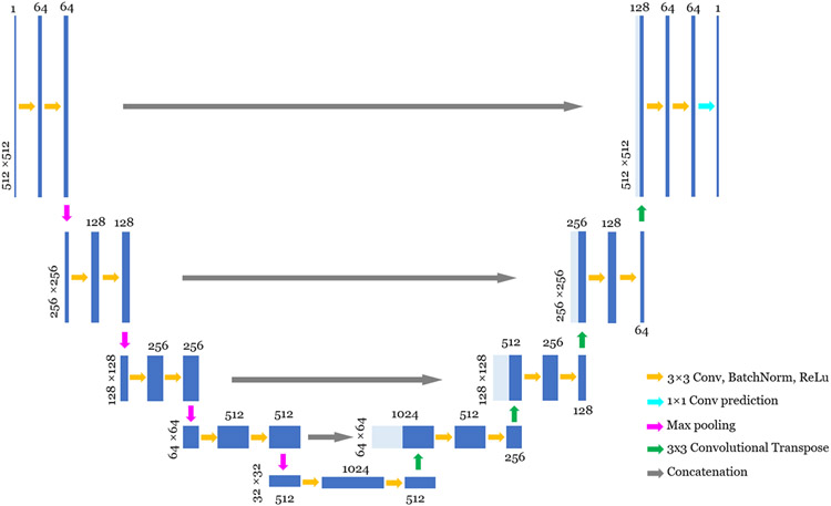
The workflow of the proposed DL-PICCS is presented in Figure 1. The workflow begins with the conventional FBP reconstruction of undersampled sinogram data. A deep neural network (U1) is trained to mitigate sparse-view aliasing artifacts and produce an image with reduced streaks and noise. This image is denoted as “U1-only” in Figure 1. In this work, a modified version of U-Net⁵⁴ shown in Figure 2 is employed to accomplish this task. However, one can choose any preferred neural network architecture in the proposed DL-PICCS workflow. The primary purpose of the deep neural network U1 is to eliminate sparse-view aliasing artifacts while preserving image details. Therefore, this module can be considered as a heavy-duty aliasing artifact removal module.

FIGURE 1.

Workflow of the proposed DL-PICCS framework

FIGURE 2.

Illustration of the detailed architecture of U-Net used in this work. The operations are described bottom-right. Images are represented by blue blocks with their height as image dimension and their width as channels. Concatenated images are shown in light blue. The actual image dimension is displayed on the side of the image, and the channel numbers are displayed either on the top of the image

The output of the U1 network is then used as the prior image in the PICCS reconstruction framework to reconstruct the PICCS image using both the prior image produced from the U1 network and also the sparse-view sinogram data for each individual patient. The output of PICCS reconstruction is denoted as “PICCS-U1.” The primary purpose of the PICCS reconstruction module is to accomplish accurate reconstruction for each individual patient by invoking the data fidelity term.

With the proper choice of reconstruction parameters in PICCS, as presented in the next subsection, both high accuracy and streaky artifact reduction can be reached in the PICCS-U1 image to improve reconstruction accuracy in individual patient image reconstruction. However, the noise texture and noise level in PICCS-U1 images may not be ideal for medical diagnoses. To improve noise texture and noise level for the PICCS-U1 output, another deep neural network architecture, “U2,” is trained to improve the noise texture and noise level of the PICCS output. The final output is referred to as U2-PICCS-U1, that is, DL-PICCS.

In summary, a divide-and-conquer strategy is used in DL-PICCS to comprehensively address the encountered challenges in the sparse-view CT reconstruction problem: deep learning U1 module to eliminate streaking artifacts, PICCS module to improve reconstruction accuracy for individual patients, and deep learning U2 module to tune noise texture and noise level in the final image.

2.2 ∣. Brief review of PICCS: Algorithm and pseudocode

The PICCS reconstruction framework¹³ can be formulated as an unconstrained problem with a parameter λ, weighting the data fidelity and regularizer terms,⁵⁵

$$\begin{gathered} \widehat{\mathbf{x}}=\underset{\mathbf{x}}{\text{arg}\text{min}}[\frac{\lambda }{2}\Vert \mathbf{A}\mathbf{x}-\mathbf{y}{\Vert }_{\mathbf{D}}^2+ \\ (\alpha \Vert {\Psi }_1(\mathbf{x}-{\mathbf{x}}_{\mathbf{p}}){\Vert }_1+(1-\alpha )\Vert {\Psi }_2(\mathbf{x}){\Vert }_1)]. \end{gathered}$$ (2.1)

Here, $\widehat{\mathbf{x}}$ denotes the reconstructed CT image, x_p denotes the prior image, y denotes the sinogram data, A denotes the system matrix, and D denotes the statistical weighting. Ψ₁ and Ψ₂ represent sparsifying transform operators and ∥ · ∥₁ denotes the L₁ norm of the image vectors. In this work, Ψ₁ and Ψ₂ are selected to be the gradient operators and the total variation (TV) norm of the image object is used to implement the L₁ norm operations. The parameter α ∈ [0, 1] controls the relative weights between the prior image and TV terms. When α = 0, the reconstruction method reduces to the TV-based SIR (TV-SIR) method.⁵⁶

Many different numerical solvers can be used to solve the unconstrained problem in Equation (1). In this work, we present a solver that has not been formally published for PICCS reconstruction. This solver uses the well-known forward-backward proximal splitting scheme⁵⁷ to split the unconstrained convex optimization problem into two subproblems: The first one is to obtain an intermediate image from the data fidelity term only, and then, this intermediate image is processed in the standard denoising problem using proximal operators with the regularizer in the PICCS objective function shown in Equation (1). The denoising problem is solved using the well-known alternating direction method of multipliers (ADMMs) scheme.⁵⁸ To facilitate potential third-party result reproduction, the pseudocode of the final solver is presented in the Supporting Information. For a detailed derivation of the solver, one can follow the mathematical steps presented in the Appendix of Ref. 59, but with the PICCS regularizer using total variation as its sparsifying transforms as a replacement for the TV regularizer in Ref. 59.

2.3 ∣. Curation of training data sets and performance evaluation data sets

All the training data used in this work were generated from numerical simulations of human subject CT image volumes by numerical forward projection operations. A total of 9765 CT image slices from 30 cases of abdomen and contrast-enhanced chest CT exams were used to generate sinogram data for training, validating, and testing purposes. Among the 9765 image slices, we selected 8483 image slices from 26 patient cases to generate data for training and 834 slices from two patient cases for validation purposes, whereas the remaining 448 images slices from two patient cases were used to generate the data set for test and performance evaluation purposes. U1 was trained with paired undersampled FBP and ground truth data and U2 was trained with paired PICCS-U1 output and ground truth data.

The standard ray-driven numerical forward projection procedure⁶⁰ was used to produce the sinogram data using a fan-beam geometry. To facilitate the performance evaluation (described in next subsection) from clinical cases acquired from a 64-slice CT scanner (Discovery CT750 HD, GE Healtcare, Waukesha), all the simulation data generation used the same scanner geometry: detector size, source-to-detector distance, and source-to-isocenter distance. Poisson noise was added to the simulated sinogram data. The noise level in each CT image is determined by the total photon number, that is, total fluence (TF) level, delivered to the subject in each CT data acquisition and the total photon number is determined by the number of view angles (N_Angle) and entrance photon fluence (I₀, unit: counts) at each view angle, that is, TF = N_Angle × I₀ with counts as the unit. In this study, N_Angle ∈ {984, 123, 82} and four entrance photon fluence levels were used: standard dose (I₀ = 1.0 × 10⁶), moderate dose (I₀ = 5.0 × 10⁵), low dose (I₀ = 3.0 × 10⁵), and ultralow dose (I₀ = 1.0 × 10⁵). This choice of entrance photon fluence level is to roughly match the noise level in the FBP reconstructed image with N_Angle = 984 for the aforementioned 64-slice CT scanner: 35 HU (standard dose), 45 HU (moderate dose), 66 HU(low dose), 90 HU (ultralow dose). For later references, the four TF levels were kept the same for both the 123-view and 82-view acquisitions and are given in Table 1. In both cases, the notation TF₁ is reserved for the noiseless case.

TABLE 1.

Summary of four total fluence levels (unit: counts)

	Standard dose	Moderate dose	Low dose	Ultra-low-dose
	TF2(×106)	TF3(×105)	TF4(×105)	TF5(×105)
Entrance fluence/view	1.0	5.0	3.0	1.0
Total fluence 123-view	123 × 1.0	123 × 5.0	123 × 3.0	123 × 1.0
Total fluence 82-view	82 × 1.5	82 × 7.5	82 × 4.5	82 × 1.5

2.4 ∣. Numerical implementation details

FBP reconstruction was performed for each TF setting using an image matrix of 512 × 512 and a reconstruction field-of-view (FOV) of 40 cm diameter.

The FBP-reconstructed images for 123-view and 82-view angle images were paired with the corresponding FBP-reconstructed images from 984 view angle images at each entrance photon fluence level to form training data pairs and used to train the U1 module shown in Figure 1.

PICCS reconstruction was performed using the pseudocode presented in the Supporting Information and the reconstruction parameters are presented in the following Table 2. The PICCS reconstruction parameters listed in Table 2 were empirically optimized to achieve natural noise texture in visual perception. The stopping criterion for the PICCS reconstruction was set as the relative changes between two iterations, that is, $\frac{\Vert x_{n+1}-x_n\Vert }{\Vert x_n\Vert }\le 0.009$.

TABLE 2.

Parameters for PICCS reconstruction in DL-PICCS framework

	Parameters	TF1	TF2	TF3	TF4	TF5
123-view	ν	0.70	0.70	0.70	0.70	0.70
	α	0.71	0.71	0.71	0.71	0.71
	μ	5.0 × 10−5	8.0 × 10−4	2.1 × 10−3	2.2 × 10−3	5.0 × 10−3
	λ	2.5	12	15	15	4
	N d	30	30	30	30	30
82-view	ν	0.70	0.70	0.70	0.70	0.70
	α	0.71	0.71	0.71	0.71	0.71
	μ	6.0 × 10−5	6.0 × 10−4	2.0 × 10−3	3.0 × 10−3	3.0 × 10−3
	λ	3	5	15	14	3
	N d	30	30	30	30	30

The network training of U1 and U2 utilized the same strategy, using the Adam optimizer with β = 0.5, learning rate of 1 × 10⁻⁴, which was decreased to 10⁻⁵ after 50 epochs, for a total of 60 epochs. The loss function uses the mean absolute error (L1 Loss), which can be described in the following form:

$$\text{Loss}=\frac{1}{\mathrm{N}}\sum _{\mathrm{i}=1}^{\mathrm{N}}\mid {\mathrm{x}}_{\text{output},\mathrm{i}}-{\mathrm{x}}_{\text{target},\mathrm{i}}\mid ,$$

where N represents the number of data points in the training data cohort. x_output,i denotes the network output image and x_target,i denotes the target image.

2.5 ∣. Generalizability test (I): From numerical simulation to clinical human subject data

Both the U1 and U2 deep neural network architectures in DL-PICCS were trained using numerical simulation data described in Section 2.3. These simulations were performed at very precise view angle positions and only trained over four different radiation exposure levels. Therefore, if the trained U1 and U2 modules are directly applied to reconstruct images from actual clinical patient cases, that is, the sinogram data acquired from clinical CT scanners, one would not expect accurate image reconstruction for the individual human subject. To test the generalizability of the simulation data-trained U1 and U2 modules to perform clinical data reconstruction, data from abdominal CT exams under the Institutional Review Board (IRB) approval were retrospectively extracted from a 64-slice multirow detector CT (Discovery CT 750HD, GE Healthcare, Waukesha) to test the proposed DL-PICCS reconstruction performance at 123-view angle condition. Note that the clinical CT scans produce 984 view angles in the sinogram, we retrospectively parsed the fully sampled sinograms into the corresponding 123-view angle sinograms for performance evaluation purposes.

The difficulty of this generalizability test lies in the changes of data acquisition conditions from the training data of the U1 and U2 modules to the actual clinical data that are summarized as follows:

1. The starting view angles in experimental data are different from those in training. Hence the orientation of streak artifacts of the testing experimental data sets is different from that of the training data.

2. The potential inclusion of external objects, for example, contrast injection devices and ECG, yields different streaking artifact patterns. Particularly, the streaks originating from the external objects are more dominant.

3. Experimental data have different noise conditions (the noise condition in Human 2 roughly corresponds to the moderate-dose level in training with noise standard deviation of 45 HU measured in a uniform region. Human 1 and 3 are noisier with noise standard deviation of 70 HU in uniform regions, which is considered as low-dose scans in clinical practice).

4. CT couch also changes data conditions if it is not represented in training data.

2.6 ∣. Generalizability test (II): Replacement of the U1 module by a different trained network in DL-PICCS

To further test the generalizability of the proposed DL-PICCS framework, the following question needs to be addressed: Can one replace the U1 module by another deep neural network architecture trained by external researchers? The difficulty of the test lies in the fact that the training data set can be very different from the performance test data because the U1 module will be trained by different people, and thus, the data acquisition conditions of the training data can be dramatically different from the test data.

To answer this question for the generalizability test of the proposed DL-PICCS method, we replaced the U1 module with a network trained by another group and made publicly available: the tight-frame U-Net¹⁶ (https://github.com/hanyoseob/framing-u-net). Note that the available tight-frame U-Net was trained using simulated parallel-beam CT data and 120 view angles, whereas the actual test cases described in Section 2.5 were acquired in a cone-beam geometry with 123 view angles and with totally different noise conditions. It is expected that the direct generalization from the trained tight-frame U-Net to our clinical data set will not work well. Therefore, the real question is whether the proposed DL-PICCS method will help correct the output of the trained tight-frame U-Net for clinically accurate reconstruction? In this work, we refer to the tight-frame U-Net as TightU. Also to avoid confusion, we refer to DL-PICCS with only U1 replaced by TightU as U2-PICCS-TightU.

2.7 ∣. Quantitative reconstruction accuracy evaluation metrics

To quantify the reconstruction accuracy, two standard quantitative metrics, for example, relative root mean square error (rRMSE) and structural similarity index metric (SSIM)⁶¹ are used in this paper. These metrics are defined as follows:

$$\text{rRMSE}(x,x_0)=\frac{\Vert x-x_0{\Vert }_2}{\Vert x_0{\Vert }_2}\times 100\%,$$ (2.2)

where x denotes the reconstructed image and x₀ denotes the ground truth or reference image.

$$\text{SSIM}(x,x_0)=\frac{(2{\mu }_x{\mu }_{x_0}+a_1)(2{\sigma }_{x,x_0}+a_2)}{({\mu }_x^2+{\mu }_{x_0}^2+a_1)({\sigma }_x^2+{\sigma }_{x_0}^2+a_2)},$$ (2.3)

where μ_x denotes the mean value of image x, σ_x denotes the variance of x, and similar properties are defined for the reference image x₀. σ_x,x0 denotes the covariance of x and x₀. a₁ = 1 × 10⁻⁶ and a₂ = 3 × 10⁻⁶ are two constants that are used to stabilize the division with a small value in the denominator. To calculate the sample mean and variance used in the above formula, we use an 11 × 11 circularly symmetric Gaussian weighting function with a standard deviation of 1.5 pixels, normalized to a unit sum.⁶¹ The full FOV of an image was used to calculate all quantification metrics.

Besides the quantitative performance evaluation, noise textures and clinically relevant lesions were also qualitatively assessed in zoomed-in images. The magnified images can help to visually inspect false positive and false negative lesions in reconstructed images.

3 ∣. RESULTS

3.1 ∣. Quantitative reconstruction accuracy of DL-PICCS: Compared with ground truth in numerical simulation test data set

To assess the reconstruction accuracy of the proposed DL-PICCS, the 448 image slices in the test data cohort generated in numerical simulations were reconstructed and compared against the ground truth images that were reconstructed from the fully sampled sinogram data with 984 view angles using the FBP algorithm.

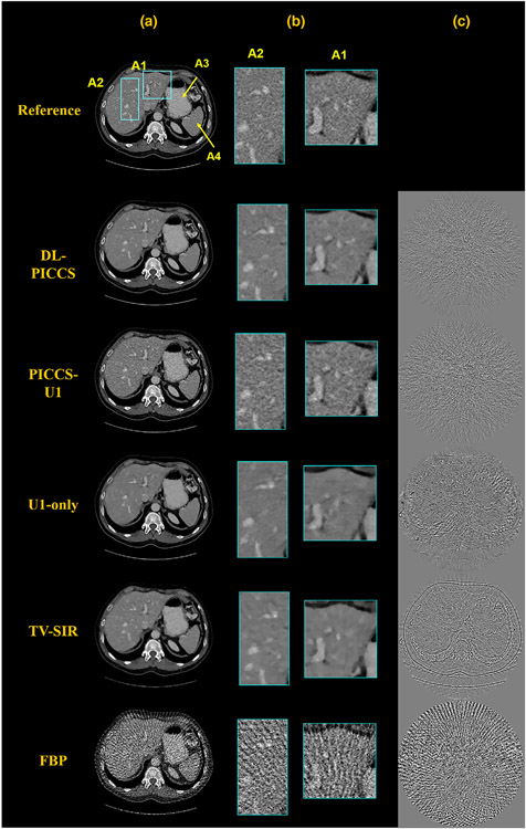
Figure 3 shows the reconstruction results of a representative sinogram with 123 views at the moderate dose level, reconstruction results from direct FBP reconstruction, from U1 module (U1-only), from PICCS with U1 output as the prior image (PICCS-U1), and then further refined image by U2 module (DL-PICCS). For comparison, the same data were also reconstructed using TV-SIR with setting α = 0 in PICCS. The implementation of TV-SIR was optimized to achieve the best rRMSE compared with ground truth with the parameter α = 0. As one can observe in Figure 3, the streaking artifacts present in the stomach (indicated by A3) and spleen (indicated by A4) regions were removed in the U1-only image, and the residual edges in the U1-only image were reduced in PICCS-U1 image, and finally, the noise level in PICCS-U1 image is further reduced in the DL-PICCS image. As a comparison, TV-SIR reconstruction indeed eliminated streaking artifacts and reduced noise levels as one expects from CS-type reconstructions. However, residual image edges are clearly observed in the TV-SIR difference image.

FIGURE 3.

Moderate-dose reconstruction pipeline of the liver CT case using 123-view sinogram data. Column (a) reconstructed images; (b) zoomed-in images; and (c) difference images. Display window W/L: 400/50 HU; Residual image display window W/L: 200/0 HU

Zoomed-in regions labeled by A1 and A2 highlight the low-contrast hepatic portal veins. Both anatomical regions were precisely reconstructed in PICCS-U1 and DL-PICCS with greatly reduced background streaks and noise. Visual perception also demonstrates that DL-PICCS restored the distorted low-contrast objects in terms of the shape, size, and contrast, eliminated the residual streaks compared with U1-only, and reduced uniform noise level in the PICCS-U1 images.

Quantitative reconstruction accuracy results are presented in Table 3. As shown in the results, DL-PICCS reconstruction shows the best reconstruction accuracy as quantified by both quantitative image quality evaluation metrics: rRMSE and SSIM.

TABLE 3.

Quantitative analysis for simulation studies using 123-view moderate-dose data

Case	Method	rRMSE(%)	SSIM
Liver	DL-PICCS	2.69	0.973
	PICCS-U1	3.20	0.962
	U1-Only	3.27	0.965
	TV-SIR	3.80	0.959
	FBP	13.40	0.610
Upper GI	DL-PICCS	2.20	0.979
	U1-only/UNet	2.63	0.972
	PICCS-U1	2.59	0.971
	TV-SIR	3.32	0.964
	FBP	11.60	0.641

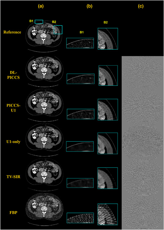
Results regarding the generalization of DL-PICCS to other anatomical structures are presented in Figure 4. Figure 4 shows an example for upper gastrointestinal (GI) CT imaging. It can be observed that major GI structures and detailed small structures such as the vessels in the upper peripheral fat region (zoomed-in by B1), the details in the muscle on the right side of the image (zoomed-in by B2), were well reconstructed in PICCS-U1 and DL-PICCS images. Compared with PICCS-U1, DL-PICCS shows improved noise performance. However, the U1-only method and TV-SIR missed vessels in B1 and the muscle details in B2. Quantitative results are presented in Table 3 and demonstrates that DL-PICCS can be effective and robust when applied to reconstruction of different anatomical structures.

FIGURE 4.

DL-PICCS reconstruction pipeline of an upper GI image slice under moderate-dose condition using 123-view sinogram data. Column (a) reconstructed images; (b) zoomed-in images specified by B1 and B2; and (c) difference images. Display window W/L: 350/50 HU. Difference image display window W/L: 200/0 HU

3.2 ∣. Change of reconstruction accuracy under different dose conditions

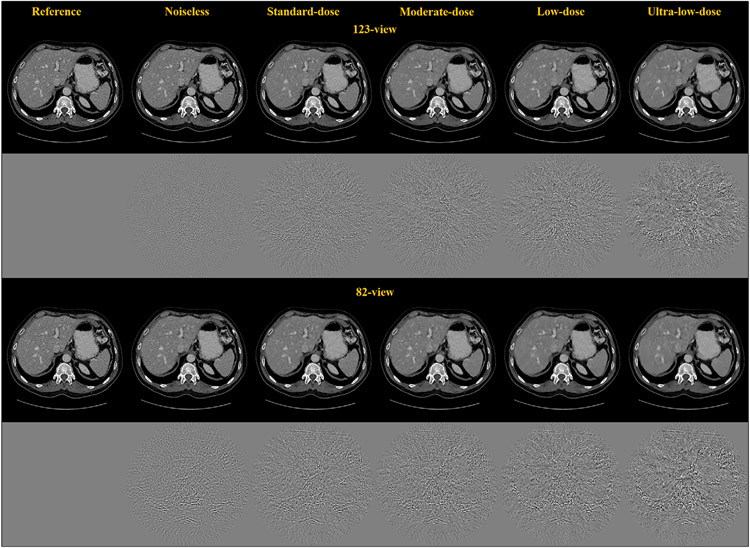
To study how the reconstruction accuracy of DL-PICCS changes with different radiation dose levels, images at different TF) levels were reconstructed at a fixed number of view angles. Figure 5 presents the DL-PICCS reconstructed abdominal images with the liver present under five different dose conditions for the 123-view case and the 82-view case. As one can visually observe, as the dose level is reduced, reconstruction accuracy drops. As a result, some low-contrast content cannot be accurately restored and unnatural noise textures begin to appear if the radiation dose is too aggressively reduced. Therefore, for any reconstruction scheme, it is important to map out the potential working conditions for the algorithm. There is no exception for the proposed DL-PICCS.

FIGURE 5.

Undersampling reconstruction under different TF levels for both 123-view and 82-view DL-PICCS reconstruction. As the TF level becomes lower, the performance of DL-PICCS degrades. Display window W/L: 400/50 HU. Residual image display window W/L: 200/0 HU

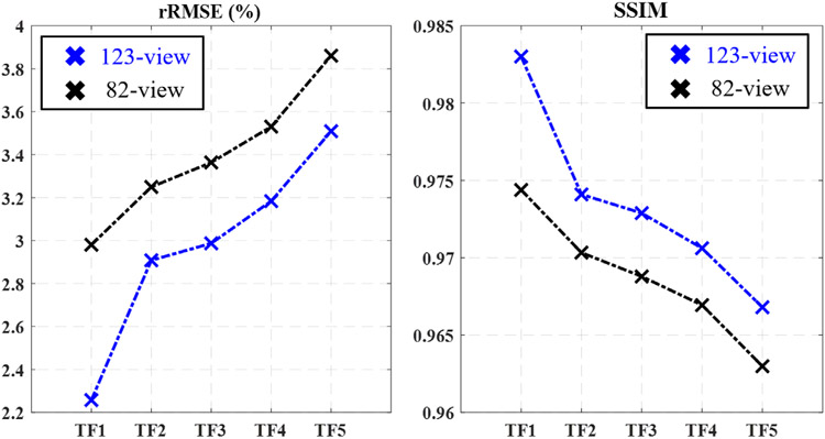
The quantitative reconstruction accuracy at different dose levels has been studied for DL-PICCS at both the 82-view and 123-view cases and the results are presented in Figure 6. As shown in both rRMSE and SSIM plots, when the radiation dose level is reduced, the quantitative reconstruction accuracy drops. For a specific clinical diagnostic task, the requirement of reconstruction accuracy can also be different. Therefore, it is difficult to set a universal purpose hard-threshold for reconstruction accuracy. However, for a given selection of reconstruction accuracy, the quantitative results shown in Figure 5 can help determine the optimal dose level.

FIGURE 6.

Dependence of DL-PICCS reconstruction accuracy on TF levels and the number of view angles

3.3 ∣. Generalizability test (I): From simulation trained network to clinical human subject data

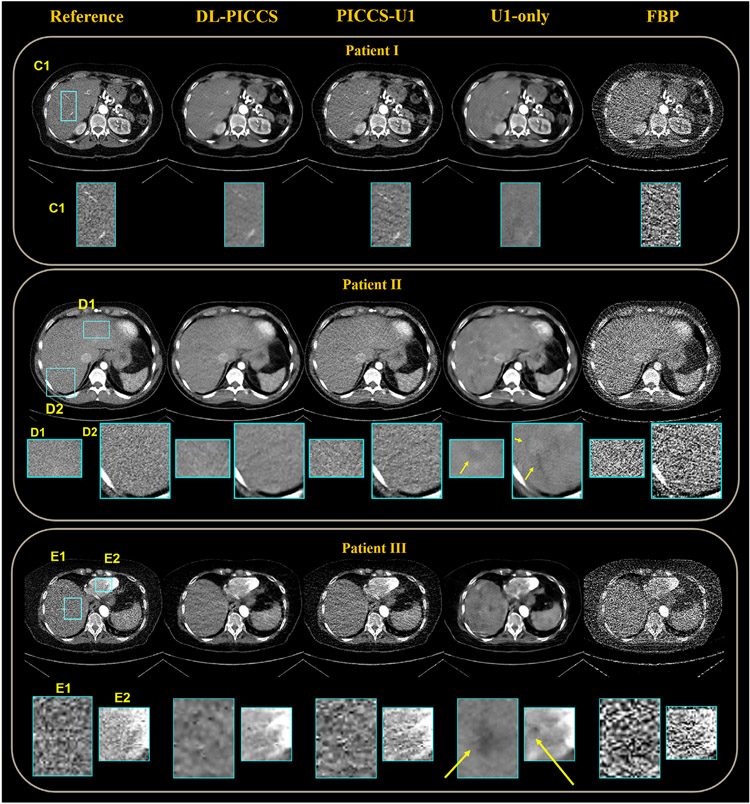
To test generalizability, the trained U1 and U2 modules using numerical simulation data were used in the proposed DL-PICCS to reconstruct three human clinical cases. Results of 123-view reconstruction are presented in Figure 7. The reference images were reconstructed from FBP using all 984 view angles.

FIGURE 7.

Reconstruction pipeline of three real human abdomen cases using 123-view sinograms. Four stages of reconstruction are specified and their zoomed-in images, C1, D1, D2, E1, E2, are below. Display window W/L: 400/50 HU. Residual image display window W/L: 200/0 HU

As shown in all three clinical cases, while the U1-only image can effectively eliminate sparse-view streaking artifacts and significantly reduce noise in FBP images, potential generalizability issues resulting from the statistical regression nature of deep learning methods are also clearly shown in the U1-only images. As shown in the zoomed-in images of the first subject, the two hepatic veins of the liver in region C1 are removed in the U1-only image. In the DL-PICCS image, not only are the hepatic veins restored, but also the noise texture and noise level are significantly improved compared to the PICCS-U1 reconstruction. In the second subject, a false positive lesion is generated in the U1-only image, distorted and generated structures are present in the zoomed-in uniform regions in the liver as indicated by the yellow arrows. In contrast, the final output from DL-PICCS removed those false positive structures in the D1 and D2 regions. Overall, the DL-PICCS images restored the correct anatomical structures and eliminated most of the noise and streaking artifacts present in the FBP images and PICCS-U1 images. In the third clinical case, the U1-only image failed in reconstructing the liver as multiple lesion-like objects are present while they are not present in the reference image shown by the zoomed-in areas E1 and E2. In contrast, the DL-PICCS reconstruction successfully identified and removed these false positive lesions.

3.4 ∣. Generalizability test (II): Replacement of U1 network in DL-PICCS

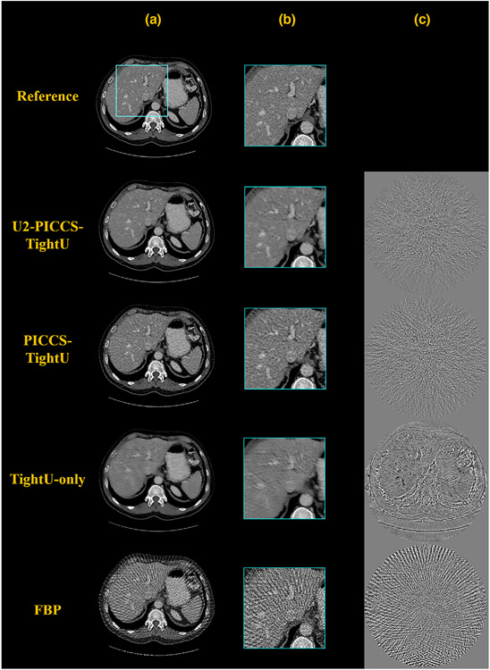
To further challenge the generalizability of DL-PICCS, the U1 segment was replaced by the publicly available trained TightU to process the numerically simulated cases presented in Figure 3. As shown in Figure 8, it is actually amazing to see how well the tight-frame U-Net performed in this extremely challenging test. Most of the sparse-view streaking artifacts in the FBP reconstruction were eliminated by TightU, although the reconstruction accuracy is not ideal as shown in the difference image. Residual edges for large and small anatomical structures are present in the difference image indicating the reduced reconstruction accuracy and degraded spatial resolution. When the TightU-only image is further processed with PICCS to produce the PICCS-TightU image, the reconstruction accuracy is improved and the final results with U2-PICCS-TightU are further improved. The quantitative reconstruction accuracy was studied and results are presented in Table 4.

FIGURE 8.

DL-PICCS reconstruction pipeline, replacing U1 with TightU. The example shows a 123-view reconstruction of the liver. Column a) reconstructed images; b) zoomed-in images; c) difference images. The output of TightU is decent, but suffered from a slight loss of resolution and structure. It served as the prior image in DL-PICCS framework. The final outcome of DL-PICCS in the zoomed-in area restored the resolution and the veins with natural noise texture. Display window W/L: 400/50 HU. Residual image display window W/L: 200/0 HU

TABLE 4.

Quantitative analysis for generalizability test (II): DL-PICCS reconstruction with U1 replaced by TightU

Case	Method	rRMSE(%)	SSIM
Liver	U2-PICCS-TightU	2.81	0.971
	PICCS-TightU	3.95	0.945
	TightU-Only	3.86	0.953
	FBP	13.40	0.610

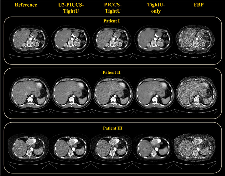
The same generalizability test was then applied to the human subject cases to test whether DL-PICCS is able to reconstruct clinically acceptable images in clinical cases. As one can visually observe in Figure 9, U2-PICCS-TightU indeed improves the reconstruction quality for TightU and PICCS-TightU, showing the improved reconstruction accuracy and improved generalizability.

FIGURE 9.

Reconstruction pipeline of three real human abdomen cases using 123-view sinograms, replacing U1 with its counterpart TightU. Four stages of reconstruction are specified. Display window W/L: 400/50 HU. Residual image display window W/L: 200/0 HU

3.5 ∣. Ablation studies of the proposed DL-PICCS workflow

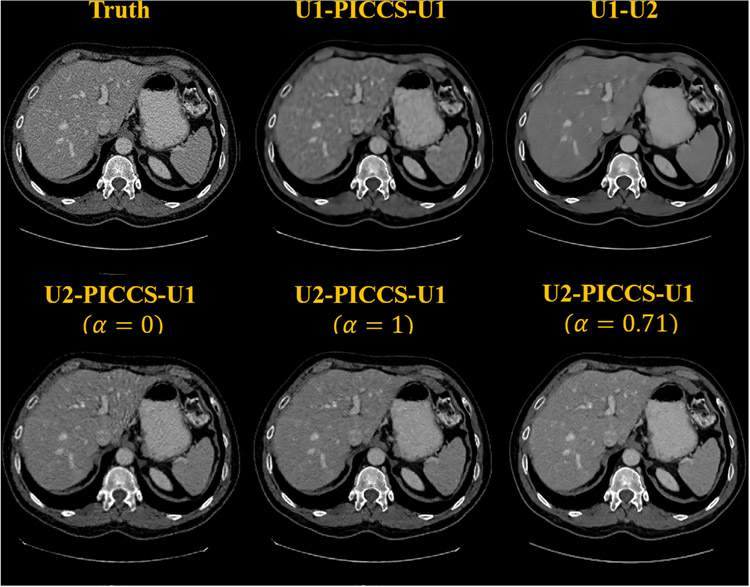
In the proposed DL-PICCS workflow, as emphasized in the design rationale, it is a divide-and-conquer strategy that has been used to eliminate streaking artifacts and to reduce the final noise level. One may wonder whether the same trained network U1 with streak-elimination functionality can also be applied to perform noise reduction in the place of U2. As shown in Figure 10 denoted by U1-PICCS-U1, without further network parameters optimization, it is clear that the reconstructed image is overly smooth due to the use of the heavy-duty U1 rather than the light-duty U2 network. To demonstrate the role played by PICCS in the proposed DL-PICCS workflow, as shown in Figure 10, the PICCS reconstruction step is eliminated from the DL-PICCS workflow to generate the result of U1-U2. It can be observed that the simplified U1-U2 reconstruction generates blurred low-contrast structures and eliminates some important image features. Finally, to demonstrate the potential importance of the weighting factor, that is, the strength parameter α in PICCS, the reconstruction results from two extremal values, α = 0.0 and α = 1.0, are also presented in Figure 10. As one can clearly observe, residual streaking artifacts emanating from the center to the peripheral are clearly visible and the noise level is also high in the α = 0.0 case, that is, if the streak-free prior image is not used. In contrast, when α = 1.0 is chosen, some subtle hepatic veins in the reconstructed images are blurred when they are compared to the empirically optimized case of α = 0.71 as suggested in this work.

FIGURE 10.

Reconstruction examples of different configurations of DL-PICCS modules on the first row and different selections of prior image weight in the second row. Display window W/L: 400/50 HU

4 ∣. DISCUSSION

In this work, deep learning reconstruction strategies were combined with PICCS to address the reconstruction accuracy and generalizability issues present in current deep learning-only image reconstruction strategies for sparse-view CT reconstruction problems. The results demonstrate the following findings: (1) When a deep learning reconstruction method was applied to reconstruct sparse-view CT data, the reconstructed images were subject to structural loss and distortion, residual streaks, and degraded spatial resolution. When the proposed DL-PICCS is applied, reconstruction accuracy is improved with better noise texture, and elimination of streaks while preserving the low-contrast veins in the liver. (2) The U1 and U2 networks trained with numerical simulation data can be directly applied to experimental data sets with very different data conditions, including different starting view angles, different undersampling patterns, and different noise levels, without significant degradation in reconstruction accuracy. (3) The U1 network can even be replaced by other trained networks available with similar functionality, as long as the sparse-view aliasing artifacts can be effectively eliminated by the replaced network architecture, the proposed DL-PICCS is able to reconstruct images with improved reconstruction accuracy to enhance the generalizability of the U1 network.

There are several other limitations of this work. First, the number of test cases are limited, it is important to test the performance of the proposed DL-PICCS more extensively over a large cohort of patients. Second, the data acquisition conditions are still limited to step-and-shoot circular acquisitions, it remains to be investigated how well the proposed DL-PICCS works for helical data acquisition conditions. Third, implementation of the DL-PICCS is not yet optimized for reducing the total reconstruction time. Although the focus of the current work is on reconstruction accuracy and generalizability, it is also important to reduce the total processing time of the proposed DL-PICCS for future clinical tests. Fourth, there exist other possible ways to combine the deep learning reconstruction with iterative image reconstruction algorithms,^30-48,52,53 and therefore, it is interesting, but much more challenging, to compare the performance of the proposed DL-PICCS with other possible combinations in terms of reconstruction accuracy, generalizability, and reconstruction time. These more thorough comparative studies are beyond the scope of the current work. Fifth, in the current DL-PICCS framework, a consistency check between the output of U2 and the measured projection data was not performed, as it was for the output of U1. This choice was due to the fact that the primary purpose of the U2 module is to perform light-duty noise reduction, and thus, the additional consistency check may bring noise back into the reconstructed image from the high-noise projection data. Additionally, we did not perform generalizability test for the U2 module due to the above design objective: a light-duty module to slightly reduce noise. Therefore, we did not anticipate any severe challenges in its generalizability. However, in specific applications, the generalizability of the U2 module should be monitored and model fine-tuning should be performed whenever it is necessary. Finally, the U1 and U2 modules in the current DL-PICCS implementations were trained separately, one can also perform end-to-end training for the entire DL-PICCS pipeline. The PICCS reconstruction step can be treated as a frozen module that does not impact the backpropagation step in the network training process.

5 ∣. CONCLUSION

In conclusion, deep learning-only reconstruction methods have intrinsic limitations in reconstruction accuracy and generalizability to individual patients due to the regression nature of the method. The combination of deep learning methods with the previously published PICCS offers a promising opportunity to achieve personalized reconstruction with improved reconstruction accuracy and enhanced generalizability.

DATA AVAILABILITY STATEMENT

The data that support the findings of this study are available from the corresponding author upon reasonable request.

REFERENCES

- 1.Leng S, Zambelli J, Tolakanahalli R, et al. Streaking artifacts reduction in four-dimensional cone-beam computed tomography Med Phys. 2008;35:4649–4659. [DOI] [PMC free article] [PubMed] [Google Scholar]
- 2.Leng S, Tang J, Zambelli J, Nett B, Tolakanahalli R, Chen G-H. High temporal resolution and streak-free four-dimensional cone-beam computed tomography Phys Med Biol. 2008;53:5653–5673. [DOI] [PMC free article] [PubMed] [Google Scholar]
- 3.Chen G-H, Theriault-Lauzier P, Tang J, et al. Time-resolved interventional cardiac C-arm cone-beam CT: an application of the PICCS algorithm. IEEE Trans Med Imaging. 2012;31:907–923. [DOI] [PMC free article] [PubMed] [Google Scholar]
- 4.Hansis E, Schafer D, Dossel O, Grass M. Evaluation of iterative sparse object reconstruction from few projections for 3-D rotational coronary angiography. IEEE Trans Med Imaging. 2008;27:1548–1555. [DOI] [PubMed] [Google Scholar]
- 5.Flohr TG, Leng S, Yu L, et al. Dual-source spiral CT with pitch up to 3.2 and 75 ms temporal resolution: image reconstruction and assessment of image quality. Med Phys. 2009;36:5641–5653. [DOI] [PubMed] [Google Scholar]
- 6.Lewis MA, Pascoal A, Keevil SF, Lewis CA. Selecting a CT scanner for cardiac imaging: the heart of the matter. Br J Radiol. 2016;89:20160376. [DOI] [PMC free article] [PubMed] [Google Scholar]
- 7.Chen G-H, Tang J, Hsieh J. Temporal resolution improvement using PICCS in MDCT cardiac imaging. Med Phys. 2009;36:2130–2135. [DOI] [PMC free article] [PubMed] [Google Scholar]
- 8.Tang J, Hsieh J, Chen G-H. Temporal resolution improvement in cardiac CT using PICCS (TRI-PICCS): performance studies. Med Phys. 2010;37:4377–4388. [DOI] [PubMed] [Google Scholar]
- 9.Donoho DL. Compressed sensing. IEEE Trans Inf Theory. 2006;52:1289–1306. [Google Scholar]
- 10.Candès EJ, Romberg JK, Tao T. Stable signal recovery from incomplete and inaccurate measurements. Commun Pure Appl Math. 2006;59:1207–1223. [Google Scholar]
- 11.Lustig M, Donoho D, Pauly JM. Sparse MRI: the application of compressed sensing for rapid MR imaging. Magn Reson Med. 2007;58:1182–1195. [DOI] [PubMed] [Google Scholar]
- 12.Sidky EY, Pan X. Image reconstruction in circular cone-beam computed tomography by constrained, total-variation minimization. Phys Med Biol. 2008;53:4777–4807. [DOI] [PMC free article] [PubMed] [Google Scholar]
- 13.Chen G-H, Tang J, Leng S. Prior image constrained compressed sensing (PICCS): a method to accurately reconstruct dynamic CT images from highly undersampled projection data sets. Med Phys. 2008;35:660–663. [DOI] [PMC free article] [PubMed] [Google Scholar]
- 14.Goodfellow I, Bengio Y, Courville A, Bengio Y. Deep Learning, Vol. 1. MIT Press; 2016. [Google Scholar]
- 15.Jin KH, McCann MT, Froustey E, Unser M. Deep convolutional neural network for inverse problems in imaging. IEEE Trans Image Process. 2017;26:4509–4522. [DOI] [PubMed] [Google Scholar]
- 16.Han Y, Ye JC. Framing U-Net via deep convolutional framelets: application to sparse-view CT. IEEE Trans Med Imaging. 2018;37:1418–1429. [DOI] [PubMed] [Google Scholar]
- 17.Zhang Z, Liang X, Dong X, Xie Y, Cao G. A sparse-view CT reconstruction method based on combination of DenseNet and deconvolution. IEEE Trans Med Imaging. 2018;37:1407–1417. [DOI] [PubMed] [Google Scholar]
- 18.Xie S, Zheng X, Chen Y, et al. Artifact removal using improved GoogLeNet for sparse-view CT reconstruction. Sci Rep. 2018;8:1–9. [DOI] [PMC free article] [PubMed] [Google Scholar]
- 19.Xie H, Shan H, Wang G. Deep encoder-decoder adversarial reconstruction (DEAR) network for 3D CT from few-view data. Bioengineering. 2019;6:111. [DOI] [PMC free article] [PubMed] [Google Scholar]
- 20.Lee H, Lee J, Kim H, Cho B, Cho S. Deep-neural-network-based sinogram synthesis for sparse-view CT image reconstruction. IEEE Trans Radiat Plasma Med Sci. 2018;3:109–119. [Google Scholar]
- 21.Dong J, Fu J, He Z. A deep learning reconstruction framework for x-ray computed tomography with incomplete data. PLoS One. 2019;14:e0224426. [DOI] [PMC free article] [PubMed] [Google Scholar]
- 22.Li Y, Li K, Zhang C, Montoya J, Chen G-H. Learning to reconstruct computed tomography images directly from sinogram data under a variety of data acquisition conditions. IEEE Trans Med Imaging. 2019;38:2469–2481. [DOI] [PMC free article] [PubMed] [Google Scholar]
- 23.He J, Wang Y, Ma J. Radon inversion via deep learning. IEEE Trans Med Imaging. 2020;39:2076–2087. [DOI] [PubMed] [Google Scholar]
- 24.Xie H, Shan H, Cong W, et al. Deep efficient end-to-end reconstruction (DEER) network for few-view breast ct image reconstruction. IEEE Access. 2020;8:196633–196646. [DOI] [PMC free article] [PubMed] [Google Scholar]
- 25.Kang E, Chang W, Yoo J, Ye JC. Deep convolutional framelet denosing for low-dose CT via wavelet residual network. IEEE Trans Med Imaging. 2018;37:1358–1369. [DOI] [PubMed] [Google Scholar]
- 26.Kang E, Min J, Ye JC. A deep convolutional neural network using directional wavelets for low-dose x-ray CT reconstruction. Med Phys. 2017;44:e360–e375. [DOI] [PubMed] [Google Scholar]
- 27.Chen H, Zhang Y, Kalra MK, et al. Low-dose CT with a residual encoder-decoder convolutional neural network. IEEE Trans Med Imaging. 2017;36:2524–2535. [DOI] [PMC free article] [PubMed] [Google Scholar]
- 28.Chen H, Zhang Y, Zhang W, et al. Low-dose CT via convolutional neural network. Biomed Opt Express. 2017;8:679–694. [DOI] [PMC free article] [PubMed] [Google Scholar]
- 29.Wolterink JM, Leiner T, Viergever MA, Išgum I. Generative adversarial networks for noise reduction in low-dose CT. IEEE Trans Med Imaging. 2017;36:2536–2545. [DOI] [PubMed] [Google Scholar]
- 30.Yang Y, Sun J, Li H, Xu Z. Deep ADMM-Net for compressive sensing MRI. In: Lee DD, Sugiyama M, Luxburg UV, Guyon I, Garnett R, eds. Advances in Neural Information Processing Systems 29. Curran Associates, Inc.; 2016:10–18. [Google Scholar]
- 31.Hammernik K, Klatzer T, Kobler E, et al. Learning a variational network for reconstruction of accelerated MRI data. Magn Reson Med. 2018;79:3055–3071. [DOI] [PMC free article] [PubMed] [Google Scholar]
- 32.Zhang J, Ghanem B. ISTA-Net: interpretable optimization-inspired deep network for image compressive sensing. In: 2018 IEEE/CVF Conference on Computer Vision and Pattern Recognition; 2018:1828–1837. [Google Scholar]
- 33.Chen H, Zhang Y, Chen Y, et al. LEARN: learned experts’ assessment-based reconstruction network for sparse-data ct. IEEE Trans Med Imaging. 2018;37:1333–1347. [DOI] [PMC free article] [PubMed] [Google Scholar]
- 34.Schlemper J, Caballero J, Hajnal JV, Price AN, Rueckert D. A deep cascade of convolutional neural networks for dynamic MR image reconstruction. IEEE Trans Med Imaging. 2018;37:491–503, 1704.02422. [DOI] [PubMed] [Google Scholar]
- 35.Aggarwal HK, Mani MP, Jacob M. Model based image reconstruction using deep learned priors (MODL). In: Proceedings of the International Symposium on Biomedical Imaging, Vol. 2018. IEEE Computer Society; 2018:671–674. [DOI] [PMC free article] [PubMed] [Google Scholar]
- 36.Gupta H, Jin KH, Nguyen HQ, McCann MT, Unser M. CNN-based projected gradient descent for consistent CT image reconstruction. IEEE Trans Med Imaging. 2018;37:1440–1453, 1709.01809. [DOI] [PubMed] [Google Scholar]
- 37.Adler J, Öktem O. Learned primal-dual reconstruction. IEEE Trans Med Imaging. 2018;37:1322–1332. [DOI] [PubMed] [Google Scholar]
- 38.Wu D, Kim K, El Fakhri G, Li Q. Iterative low-dose CT reconstruction with priors trained by artificial neural network. IEEE Trans Med Imaging. 2017;36:2479–2486. [DOI] [PMC free article] [PubMed] [Google Scholar]
- 39.Chen B, Xiang K, Gong Z, Wang J, Tan S. Statistical iterative CBCT reconstruction based on neural network. IEEE Trans Med Imaging. 2018;37:1511–1521. [DOI] [PMC free article] [PubMed] [Google Scholar]
- 40.Liang K, Zhang L, Yang H, Chen Z, Xing Y. A model-based unsupervised deep learning method for low-dose CT reconstruction. IEEE Access. 2020;8:159260–159273. [Google Scholar]
- 41.Ding Q, Chen G, Zhang X, Huang Q, Ji H, Gao H. Low-dose CT with deep learning regularization via proximal forward–backward splitting. Phys Med Biol. 2020;65:125009. [DOI] [PubMed] [Google Scholar]
- 42.Ge Y, Su T, Zhu J, et al. ADAPTIVE-NET: deep computed tomography reconstruction network with analytical domain transformation knowledge. Quant Imaging Med Surg. 2020;10:415–427. [DOI] [PMC free article] [PubMed] [Google Scholar]
- 43.Zheng X, Ravishankar S, Long Y, Fessler JA. PWLS-ULTRA: an efficient clustering and learning-based approach for low-dose 3D CT image reconstruction. IEEE Trans Med Imaging. 2018;37:1498–1510. [DOI] [PMC free article] [PubMed] [Google Scholar]
- 44.Lempitsky V, Vedaldi A, Ulyanov D. Deep image prior. In: Proceedings of the IEEE Computer Society Conference on Computer Vision and Pattern Recognition; 2018:9446–9454. [Google Scholar]
- 45.Gong K, Catana C, Qi J, Li Q. PET image reconstruction using deep image prior. IEEE Trans Med Imaging. 2019;38:1655–1665. [DOI] [PMC free article] [PubMed] [Google Scholar]
- 46.Chun IY, Zheng X, Long Y, Fessler JA. BCD-Net for low-dose ct reconstruction: acceleration, convergence, and generalization. In: International Conference on Medical Image Computing and Computer-Assisted Intervention. Springer; 2019:31–40. [Google Scholar]
- 47.Ye S, Long Y, Chun IY. Momentum-Net for low-dose CT image reconstruction. arXiv preprint arXiv:2002.12018, 2020. [Google Scholar]
- 48.Chun IY, Huang Z, Lim H, Fessler J. Momentum-Net:fast and convergent iterative neural network for inverse problems. IEEE Trans Pattern Anal Mach Intell. 2020:1. [DOI] [PMC free article] [PubMed] [Google Scholar]
- 49.Bishop CM. Pattern Recognition and Machine Learning. Springer; 2006. [Google Scholar]
- 50.Friedman J, Hastie T, Tibshirani R. The Elements of Statistical Learning. Vol. 1, Springer Series in Statistics. Springer; 2001. [Google Scholar]
- 51.Fessler JA, Sonka M, Fitzpatrick JM. Statistical image reconstruction methods for transmission tomography. In: Kim Y, Horii SC, eds. Handbook of Medical Imaging. SPIE; 2000;2:1–70. [Google Scholar]
- 52.Hauptmann A, Lucka F, Betcke M, et al. Model-based learning for accelerated, limited-view 3-D photoacoustic tomography. IEEE Trans Med Imaging. 2018;37:1382–1393. [DOI] [PMC free article] [PubMed] [Google Scholar]
- 53.Mardani M, Gong E, Cheng JY, et al. Deep generative adversarial neural networks for compressive sensing mri. IEEE Trans Med Imaging. 2019;38:167–179. [DOI] [PMC free article] [PubMed] [Google Scholar]
- 54.Ronneberger O, Fischer P, Brox T. U-Net: convolutional networks for biomedical image segmentation. In: International Conference on Medical Image Computing and Computer-Assisted Intervention. Springer; 2015:234–241. [Google Scholar]
- 55.Lauzier PT, Tang J, Chen G-H. Prior image constrained compressed sensing: implementation and performance evaluation. Med Phys. 2012;39:66–80. [DOI] [PMC free article] [PubMed] [Google Scholar]
- 56.Tang J, Nett BE, Chen G-H. Performance comparison between total variation (TV)-based compressed sensing and statistical iterative reconstruction algorithms. Phys Med Biol. 2009;54:5781–5804. [DOI] [PMC free article] [PubMed] [Google Scholar]
- 57.Combettes PL, Pesquet J-C. Proximal splitting methods in signal processing. In: Bauschke HH, Burachik RS, Combettes PL, Elser V, Luke DR, Wolkowicz H, eds. Fixed-Point Algorithms for Inverse Problems in Science and Engineering. Springer; 2011:185–212. [Google Scholar]
- 58.Boyd S, Parikh N, Chu E, et al. Foundations and trends® in machine learning. Foundations and Trends® in Communications and Information Theory. 2011;3:1–122. [Google Scholar]
- 59.Garrett JW, Li Y, Li K, Chen G-H. Reduced anatomical clutter in digital breast tomosynthesis with statistical iterative reconstruction. Med Phys. 2018;45:2009–2022. [DOI] [PMC free article] [PubMed] [Google Scholar]
- 60.Siddon RL. Fast calculation of the exact radiological path for a three-dimensional CT array. Med Phys. 1985;12:252–255. [DOI] [PubMed] [Google Scholar]
- 61.Wang Z, Bovik A, Sheikh H, Simoncelli E. Image quality assessment:from error visibility to structural similarity. IEEE Trans Image Process. 2004;13:600–612. [DOI] [PubMed] [Google Scholar]
Associated Data
This section collects any data citations, data availability statements, or supplementary materials included in this article.
Supplementary Materials