Air circulation study inside and outside of urban buses induced by the opening of windows

Abstract

In this work, the external and internal airflow analysis in an urban bus is carried out through computational fluid dynamics. The research addresses the study of the internal flow to estimate the air change rate caused by the opening of windows. Two cases are considered: fully opening and partially opening the windows, and three bus speeds of 20, 40, and 60 km/h are assessed. The quantification of the air flow rate through the windows clearly displays that air enters through the rear windows and exits the bus through the front windows. This effect is explained by the pressure distribution in the outer of the bus, which causes the suction of the indoor air. At low bus speeds, the incoming air flow rate increases linearly with the speed, but the improvement is lower for high speeds. The theoretical air change time at 20 km/h is around 25.7 s, which is 9 times lower than expected by using HVAC systems. On the other hand, the estimation of the real air renewal time by solving a concentration shows that 40 s are needed to exchange 85% of the internal air of the bus. The research also assesses the effect of different levels of occupation inside the bus. Results are conclusive to recommend the circulation with full or partial window opening configurations in order to reduce the risk of airborne disease transmission.

Introduction

Respiratory infectious diseases have threatened public health in the last century. But, more recently, novel and high transmission viruses belonging to the Coronavirus family, such as the severe acute respiratory syndrome (SARS) in 2002–2003 (Vijayanand et al. 2004), the Middle East respiratory syndrome (MERS) in 2013 (Organization and Others 2019), and the SARS-CoV-2 (COVID-19) initiated in 2019 in China (Andersen et al. 2020) and still active around the world, have put great attention to understand the airborne virus transmission. Ballistic drop transmission, during coughing and sneezing, and indirect transmission through fomites have been well studied in many environments. However, the study of real cases allowed us to conclude that neither of these two mechanisms could explain the massive virus transmission (World Health Organization 2020). To date, the aerosols spread during talking, singing, or breeding have been unanimously defined by the scientific community as the main pathogen pathway transmission (Ou et al. 2022). Consequently, the poor ventilation and the inflow conditions have a significant effect on aerosol trajectory and virus spread.

The urban buses can transport around 40 seated passengers and a similar number of standing passengers. Although urban trips are relatively short, the public transport has been the center of discussions due to the crowding of people, the large passenger exchange rate, and the poor ventilation of some systems. The modern bus units normally include heat ventilation air conditioning (HVAC) systems with null or very low air renewal ratios. Moreover, in many buses, the windows cannot be opened. HVAC systems are very efficient from the energy point of view but at the same time, they are a potential source of virus transmission. For simplicity, typical HVAC systems are put in the center of the roof with the inlet/outlet vent grids close to the unit. During air recirculation, the air is aspirated from the cabin and passed through general-purpose mechanical filters type MERV 7/8 or ISO g3 to retain large particles. The use of high-efficiency particulate arresting (HEPA) filters is not usual in land transport media. The air is cooled or heated in evaporator units and returned to the cabin. Depending on the number of passengers or any air quality criteria, only a small fraction of external fresh air, less than 20%, is admitted for energy efficiency reasons. These compact HVAC systems placed in the center of the buses are not efficient to renew the air, especially on the rear and front sides of the buses. The HVAC without HEPA filters helps to spread aerosols, although reduces the local concentration around the emitter. To improve the air quality two options are possible: to install HEPA filters and to increase the fresh air renewal ratio. Both options are expensive and demand time to be implemented. In the short and middle time, the opening of windows, although reducing comfort, seems to be the best choice. In this sense, several countries have recently recommended or committed to the transport companies to operate by opening the windows even during cold seasons (CDCP 2021; European Commission 2020; UK 2021).

Before 2019, most scientific works regarding air quality were focused on the quantification of volatile organic compounds (VOCs), Benzene, Toluene, and the three Xylene isomers (BTEX) (Batterman et al. 2002; Hsu and Huang 2009; Parra et al. 2008). The study of comfort conditions was also addressed in several works on trains (Zhao et al. 2022), airplanes (You et al. 2019), and buses (Chan et al. 2002). But in the last 2 years, the SARS pandemic put major interest on the airborne transmission of pathogen-laden droplets (Noorimotlagh et al. 2021). Recently, Zhang et al. (2021) studied experimental and numerical techniques on the propagation of particle-laden transport inside a typical school bus. They compared the air renewal ratios during normal trips with HVAC, and with the windows opening and closing, and concluded that the HVAC uniformly distributes the aerosols throughout the bus while simultaneously diluting the concentration with fresh air. But the major conclusion was that the opening of doors and windows reduces the concentration by approximately one-half, albeit its benefit does not uniformly impact all passengers on the bus due to the recirculation of airflow. They also concluded that well-fitted surgical masks used by all passengers could nearly eliminate the transmission of the disease. Although the average improvement in indoor conditions is promoted by the opening of doors and windows, the benefit is quite dependent on the bus characteristics, location of the infected and susceptible passengers, the size of windows, and the speed of the bus among others. During window opening tests, Zhang et al. (2021) observed that the aerosol particles exhaled by a passenger standing in the bus corridor move from the rear to the front of the bus. This phenomenon was also observed by Kale et al. (2007) during miniature scaled bus experiments. In the current paper, this particular air circulation from the rear to the front is also evidenced through numerical simulation and the causes of this are explained based on the external airflow. The purpose of this paper is to study the indoor airflow patterns and to quantify the air renewal ratio obtained with different window opening configurations in a typical urban bus traveling at different speeds. To achieve that the inner and outer aerodynamics are solved. The presence of stagnation flow zones is quantified by solving the residence time of a scalar transport variable. This paper aims to provide mitigation strategies and guidelines to be implemented in a short time in order to reduce airborne disease transmission.

Governing equations

In this study, the incompressible single-phase Navier–Stokes equations are solved using the OpenFOAM-8.0 (OpenFOAM Foundation 2020) suite (open field operation and manipulation) which is a free and open source code. The Newtonian isothermal flow is mathematically described by the continuity and the momentum equation balances, which can be written in a conservative form as:

$$\mathrm{\nabla }.\underset{\_}{U}=0$$

$$\frac{\partial \underset{\_}{U}}{\partial t}+\mathrm{\nabla }.\left(\underset{\_}{U},\underset{\_}{U}\right)=\mathrm{\nabla }.\left({\sigma }_{\mathit{eff}},\mathrm{\nabla },\underset{\_}{U}\right)-\frac{1}{\rho }\mathrm{\nabla }p$$

where $\underset{\_}{U}$ is the velocity, $p$ the pressure, $\rho$ the air density, and ${\sigma }_{\mathit{eff}}$ the effective viscosity which considers the molecular and turbulent contributions. In this work, the turbulent closure equation is obtained from the Smagorinsky Large-eddy simulation (LES) model (Smagorinsky 1963), in which the subgrid-scale eddy viscosity ${\sigma }_t$ is defined as:

$${\sigma }_t=C_s^2{\mathrm{\Delta }}^2|\overline{S}|$$

where $C_s$ is the Smagorinsky constant ($C_s\approx 0.2$) and $\mathrm{\Delta }$ is the filter length scale. $|\overline{S}|$ is the magnitude of the resolved strain rate tensor. Ferziger and Peric (2001) suggested that turbulence must be properly damped close to the walls. Therefore, in this study the well-known Van Driest function (Van Driest 1956) was selected to modify the filter length scale as follows:

$$\mathrm{\Delta }=min\left({\mathrm{\Delta }}_{\mathrm{mesh}}^{1/3},,,\frac{{\kappa }^{\prime }}{C_{\mathrm{\Delta }}}\right)\left(1,-,e^{-y^{+}/A^{+}}\right)$$

where ${\mathrm{\Delta }}_{\mathrm{mesh}}$ is the cell volume, ${\kappa }^{\prime }=0.4187$ is the Von Kárman constant, and $C_{\mathrm{\Delta }}=0.158$. $y^{+}$ is a non-dimensional distance computed from the real distance from the wall ($y)$ and the near-wall friction ($u_{\tau }={\left({\tau }_w,/,\rho \right)}^{1/2}$) obtained from the wall shear stress (${\tau }_w$). The constant $A^{+}$ usually takes the value of 26. This modified filter length scale $\mathrm{\Delta }$ damps the turbulence viscosity near the walls where the turbulent viscosity should be negligible if sufficiently finer meshes are employed.

To analyze the air mixing and the presence of stagnant flow zones, the following scalar transport equation was solved:

$$\frac{\partial \gamma }{\partial t}+\mathrm{\nabla }.\left(\gamma ,\underset{\_}{U}\right)=0$$

As noted, the diffusion term is neglected because of the level of agitation inside the bus.

Computational settings

The bus geometric was built following the dimensions from a real bus commonly used in Argentina. Figure 1 displays plans of the bus studied as well as a picture of it. The bus is 11 m × 2.6 m × 3.3 m in length, wide, and height, respectively. To simulate the external flow, the bus was located into a box domain of 25 m × 16.4 m × 11 m in long, wide, and height to reduce the effect of the boundary conditions and allow the flow detachment at the rear side.

Fig. 1.

Plans and pictures of the bus

The bus has 32 seats and a capacity for around 40 standing passengers. The passengers enter through the front door and out through the rear door. There are 24 windows in the lateral walls, which can be opened giving a total opening area of around 12 m².

Three meshes with different levels of refinement were considered in order to achieve grid independence. The finest mesh was 21.57 million cells with an average cell size of 183 mm, reduced to 27 mm inside the bus. Figure 2a shows the bus domain and the name of the windows where the airflow is monitored. Figure 2b shows the finest mesh considered, which includes the inner and outer sides of the bus. Local refinement at the inner walls was needed to better represent the geometry and over the external walls of the bus in order to capture the flow detachment and the local pressure drops, especially around the front side. The meshes were made with a Hexa-Poly algorithm that creates a volume mesh from a combination of a Cartesian Hexa mesh (aligned to the global coordinate system) inside the main volumes, and a smooth transition zone towards the surface mesh made of tetra and polyhedral elements. Three zones were defined, as shown in Fig. 2b, with different levels of refinement. The maximum cell sizes were 40 mm, 68 mm, and 180 mm for zones 1, 2, and 3, respectively. Table 1 reports the main mesh characteristics. As indicated in Fig. 2, on the right, zones 1, 2, and 3 correspond to the inner side of the bus, the external side close to the bus, and the external side far front of the bus.

Fig. 2.

a bus domain and names of the windows where the airflow is monitored, b view of the volume mesh

Table 1.

Mesh parameters and difference in the average velocity through window 2 for the three meshes

Mesh	Nº of cells [× 106]	Average cell size [mm]			${\delta }^{\prime }$[%]	Velocity in W2 [m/s]	Difference [%]
		Zone 1	Zone 2	Zone 3
1	4.147	65.4	110.0	262.6	87.53	2.57	25.57
2	11.86	39.8	68.3	183.0	99.55	3.38	1.94
3	21.57	27.8	68.3	183.0	99.78	3.45	-

To represent the bus motion, a constant air velocity U_∞ was imposed to the air through the inlet patch as well as on the floor of the external box, while a free slip condition was assumed at the sides and ceil surfaces of the box. Finally, an inlet/outlet condition was applied to the outlet patch. For the bus walls, a no-slip null velocity was imposed. Regarding the pressure condition, fixed total pressure was imposed at the outlet patch, and zero gradient was chosen for the rest patches.

Unsteady runs were performed. The air flow through each open window was monitored to achieve a pseudo-steady state solution. Then, time average solutions for the velocity and pressure were obtained during a time of 30 s. This average time window was around 7 residence times for the lowest speed considered (20 km/h-5.5 m/s).

Results

In this section, the mesh independence study is first presented. Then, the airflow distribution at the inner and outer of the bus is analyzed for the bus speed of 40 km/h. Later, the effect of bus speed over the indoor air renewal is analyzed for bus speeds of 20, 40, and 60 km/h with different window open configurations.

Mesh convergence assessment

The mesh independence study was performed for the full windows opening configuration traveling at 40 km/h. Three meshes were considered, and the meshes parameters are reported in Table 1. The air velocity through window 2 (W₂ in Fig. 2) was chosen to control the convergence of the solution. Figure 3 shows the mesh convergence in terms of the time-average mean velocity through window 2. The relative difference between meshes 1 and 2 is 23%, but this reduces to only 2% between meshes 2 and 3. Therefore, mesh 2 seems to be the best option in terms of accuracy vs computational cost. Figure 3 also presents the velocity field in the vertical central plane for the three meshes in order to have an estimate of the level of refinement.

Fig. 3.

Left: average velocity through window 2 for three meshes. Right: velocity magnitude over a vertical cross-cut plane

The resolution ratio of the resolved to total turbulent kinetic energy $\delta$ (Wurps et al. 2020) was calculated in order to quantify the suitability of each mesh using LES. This parameter is calculated as the volumetric average in the domain:

$${\delta }^{\prime }=\frac{1}{V}\int \frac{k_{\mathit{res}}}{\left(k_{\mathit{res}},+,k_{\mathit{sgs}}\right)}dv$$

where $k_{\mathrm{res}}$ is the resolved kinetic energy and $k_{\mathrm{sgs}}$ is the sub-grid scale (modeled) kinetic energy. In Table 1, the average value of $\delta$ inside the bus domain is reported for each mesh.

The good guidelines for LES simulation recommend that $\gamma$ > 0.8. This criterion was achieved in most parts of the domain. Even more, the average value must be higher than 90%. That means 90% of the kinetic energy is solved. Thus, the mesh 2 resolution is enough for LES simulation with ${\delta }^{\prime }$ > 99%.

Fully windows opening case

The external flow around the fully windows opening (FWO) bus is highly turbulent with many large vortex structures. Figure 4 shows the instantaneous and time-average velocity magnitude fields over two cross-cut planes splitting the bus. The results correspond to a bus speed of 40 km/h (11.11 m/s). The comparison between both velocity fields (mean and instantaneous fields) remarks the high turbulence levels around the front and the rear side of the bus. The air impacts the front surface causing a stagnation zone just in the windshield. The air is forced to turn around the edges and detaches over the roof and the laterals. The air passing below the bus accelerates due to the contraction reaching more than 15 m/s. A low-velocity region evolves at the front of the bus and extends around half of the bus length both in the roof and lateral walls (see zone II in Fig. 4). On the other hand, downstream of zone II (zone I), the flow returns to the surface of the bus. Although it is not possible to identify the flow direction, the air flowing through the open windows is clearly observed in Fig. 4a, b, and the effect over the external flow is also relevant. The level of agitation inside the bus is quite evident in Fig. 4a.

Fig. 4.

Fully windows opening case. Velocity field: a time average velocity over a horizontal and vertical plane, b Instantaneous velocity over a horizontal and vertical plane

The pressure fields over horizontal and vertical planes splitting the bus and over the bus surface are shown in Fig. 5. As expected, the pressure increases in the front because the dynamic pressure is converted into static pressure in the stagnation zone. Over the roof and laterals in zone II, the detachment of the boundary layer causes a large region with low pressure that affects the front windows. Below the bus in the front zone, the pressure also reduces due to the local flow acceleration. The low-pressure spots close to the lateral walls in zone II correspond to the vortexes detached. The asymmetric pressure patterns in the lateral sides are due to the different number of windows on both sides.

Fig. 5.

Fully windows opening case. Pressure over vertical (a) and horizontal (b) cross-section planes splitting the bus. (c) pressure over the bus surface

The pressure around the bus laterals (see Fig. 5c) has a crucial role over the flow through the windows and the airflow inside the bus. In the middle and rear regions (zone I), the pressure is around 70 Pa higher than in the front size (zone II). Consequently, the air enters through the windows placed in zone I and leaves the bus through the windows in the front end. That is, the air inside the bus flows forward in the opposite direction to the external flow.

Comparison between full windows opening and closing cases

A fully windows closing (FWC) case was performed to visualize the effect of the opening of windows. Figure 6 shows the time-average velocity magnitude over a horizontal cut plane at the windows’ height for the closing (Fig. 6a) and opening (Fig. 6b) cases. Significant differences are evidenced in the flow outside the bus, mostly on the front side (zone II), where the detachment region is considerably greater for the FWO case. This detached flow region covers around three-quarters of the bus length. As noted in Fig. 6b, the air leaving the bus through the front windows pushes the external air layer enlarging the low-velocity region that evolves the front of the bus. On the other hand, the FWC case shows a narrow low-velocity layer, which extends until the center of the bus. The maximum velocities are found around the front corners reaching 21.2 m/s and 16.1 m/s for the FWC and FWO cases, respectively.

Fig. 6.

Time-averaged velocity over a horizontal cross-section plane on the middle of the bus: a fully windows closing case (FWC), b fully windows opening (FWO)

The drag force was monitored for both cases. A drag coefficient of 0.7022 was found for the FWC case. This high drag coefficient is expected for buses and trucks. For instance, Solmaz and İçingür (2015) performed drag force studies on an FWC bus also traveling at 40 km/h finding drag coefficients of 0.70 and 0.67 for experimental test and numerical simulation, respectively. Regarding the FWO case, the drag coefficient grew up to 0.758, which is around 8% more and directly impacts on the fuel consumption. Ali et al. (2014) performed a similar study over a simplified car geometry traveling at 45 km/h. They performed experimental tests and numerical simulations and found that the drag coefficient increased about 14.6% (numerical simulation) and 6.32% (experimental test) by opening the windows.

Internal flow with fully windows opening

The airflow inside the bus shows a high level of agitation with maximum velocities at the rear windows. Figure 7 displays the streamlines inside the bus in the top and lateral views. Although a large number of vortexes are observed, some main streamlines can be identified: the top view shows how the air enters through the windows W13 to W23 (rear side) and leaves the bus through the windows W1 to W7 (front side). In the lateral view, (a) it is worthy to note the main flow moving forwards (from the rear to the front side) close to the floor with velocities ranging from 1.5 to 2 m/s. This mainstream flow, which moves along the bus corridor, causes a large recirculation zone just behind the driver.

Fig. 7.

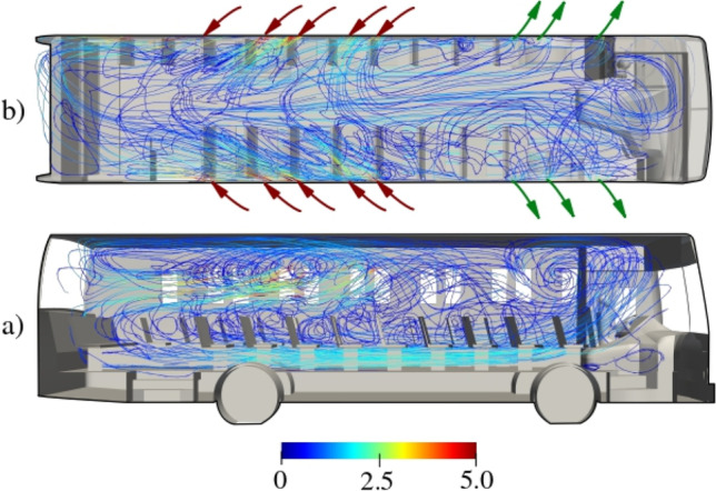
Fully windows opening case. Streamlines inside the bus: a lateral view and b top view

A secondary stream also flows forwards close to the roof with a velocity of around 1.5 m/s. In summarizing, the air flows from the rear to the front mainly close to the floor and roof of the bus. On the other hand, in the mean height zone, the flow is quite complex and highly turbulent without a clear flow direction. This unsteady turbulent flow is caused by the intermittent flow through the windows W8 to W13 placed in the central zone of the bus.

The streamlines in the top view (Fig. 7b) show a non-symmetry flow caused by the different number of windows on both sides of the bus and the influence of the baffle divisor placed at the back of the driver. Coarsely, the high velocity of the flow through the windows and the seats promotes high mixing and turbulence.

To better understand the flow inside the bus, Fig. 8 shows the time average velocity vectors in three horizontal cross-cut planes. The plane in Fig. 8a is at the middle height between the floor and the seats (y = 0.15 m from the floor). As above-mentioned, the air flows mainly along the bus corridor with velocities ranging between 1.5 and 2.0 m/s. The flow in the central zone is quite homogeneous.

Fig. 8.

Fully windows opening case. Time average velocity vectors over horizontal cross-cut planes at different heights from the floor. a y = 0.15 m, b y = 0.75 m, c y = 1.5 m

Figure 8b corresponds to a horizontal plane placed at the middle height between the seats and the windows (y = 0.75 m from the floor). Although the air is still moving forwards through the corridor, in this case large turbulent structures are clearly identified with many vortexes enclosed between adjacent seats. The air velocity remains mostly below 0.3 m/s in most places. At this intermediate height, the flow is changing from organized flow close to the floor side to high turbulent flow close to the roof side.

Figure 8c is just at the middle height of the windows (y = 1.5 m from the floor). The air enters predominantly through the rear windows with velocities up to 3 m/s (11 km/h) and leaves the bus through the front windows with velocities below 2 m/s. The windows at the center of the bus show an erratic behavior, changing the flow direction all the time. For this reason, the average velocity in zone VI is negligible. As noted, the air enters tangent to the windows in zones IV and V but exits the bus normal to the windows in zone VII.

Air velocity measurements were performed over the real bus using two-handed digital anemometers (PeakMeter-range from 0.8 to 30 m/s-sampling rate of 1 Hz with online data acquisition). The measurements were not as accurate to allow validation of the numerical results but they were useful to confirm the same general airflow patterns and verify some non-intuitive flow patterns, which were previously observed by means of simulation.

During tests, the bus was driven through a clearance straight route on a windless warm day. The bus speed was held quite constant around 40 km/h. During tests, the inlet flow and outlet flow through the rear and front windows were unquestionable evidence. On the central side, the erratic airflow direction was also visible. This is a transition region where the airflow is low and intermittent.

For a given window the velocity magnitude varied significantly in time and position, depending on the location and the orientation of the anemometer as can be inferred from the velocity vectors displayed in Fig. 8b. Due to the above-mentioned aspects, only two sample points on the central part of the corridor were included for comparison in Fig. 9, where the velocity magnitude is drawn over a vertical line from the floor to the roof. As previously mentioned, the velocity is maximum close to the floor it reduces at the middle height and increases again close to the roof. Despite the discrepancies between experimental and numerical results at the mid-height, two aspects should be remarked: firstly, the air flows always forward along the corridor. Secondly, a general agreement in the velocity profile is observed with velocity peaks close to the floor and roof sides.

Fig. 9.

Fully windows opening case. Horizontal mean velocity along a vertical line in the center of the bus corridor

Studies concerning the airflow inside vehicles with open windows are not usual and the forward direction of the flow reported in the current work has not been highlighted by others. For instance, Zhang et al. (2021) simulated the motion of aerosol particles inside an open windows bus and observed that the particles emitted by a passenger standing on the bus corridor could move to the front of the bus, but the reasons were not inferred by the authors.

Air flow rate through the windows for different opening configurations

The air flow rate through windows is presented in Fig. 10 for a bus speed of 20 km/h. This figure shows the time-average air flow rate through each window and the temporal variation (10–30 s) of eight representative windows covering the front, rear, and central zones of the bus. As noted, the air flow rates are far from constant, and the amplitude of oscillations is different for the three bus zones: for windows W1 to W6 (front side) the air is outflowing. In the second quarter (windows W7 to W12) the flow changes continuously and inverts its direction from inflow to outflow more than 10 times a minute. Despite the variations, the flow is predominantly outflowing in W7 and W8 and inflowing in W11 and W12. On the other hand, the flow through windows W13 to W18 is always inflowing and the flow variations are smaller with the average velocity around 0.23 m/s. Finally, the air through windows W19 to W22 in the rear zone is always inflowing and fluctuations are lower.

Fig. 10.

Fully windows opening case. Air flow rate through the windows (bus speed of 20 km/h)

The air flow fluctuation in each window explains the high level of agitation inside the bus. Note that some windows display a constant mean flow direction but the level of fluctuation causes transitory flow inversion.

Figure 11 shows the average flow in each window for bus speeds of 20 km/h, 40 km/h, and 60 km/h, which are common in urban buses. The air flow rate in most of the windows increases quite proportionally with the bus speed, which leads to total air flow rates of 2.3 m³/s, 4.8 m³/s, and 7.4 m³/s, respectively. This clear tendency is not observed for the windows W9 to W11.

Fig. 11.

Fully windows opening case. Air flow rate through the windows for three bus speeds

Based on the low relevance of the central windows on total air flow rate, a partial windows opening (PWO) case closing the windows W6 to W17 was carried out at a low speed of 20 km/h. The results are displayed in Fig. 12 along with the FWO case. Results are of great interest because the PWO case leads to an increment in the total air flow rate. Contrary to what was expected, a greater number of opening windows reduces the air renewal ratio. As noted in Fig. 12, the air flow rate at the open windows increases more than twice in the rear zone.

Fig. 12.

Average air flow rate through the windows with fully windows opening and partially windows opening

The results in terms of air renewal ratio are summarized in Table 2 for the four simulated cases. Considering that the bus has an internal volume of 58.7 m³, the theoretical time for fully indoor renewal can be estimated as the ratio between the internal volume and the total air flow rate. As noted, the theoretical renewal time for speeds of 20, 40, and 60 km/h are 25.7 s, 12.3 s, and 7.6 s, respectively. These times are very promising taking into account that a bus with FWC and HVAC commonly operates with air flow rates around 1 m³/s and renewal ratios of 25%. In this situation, the theoretical renewal time would grow up to 235 s, which is 9 times more than obtained by traveling with FWO at 20 km/h.

Table 2.

Incoming air flow rate and theoretical renewal time

Case	Incoming air flow rate [m3/s]	Theoretical renewal time [s]	Reduction in renewal time (%)*
FWO 20 km/h	2.3	25.7	-
FWO 40 km/h	4.8	12.3	52%
FWO 60 km/h	7.4	7.6	70%
PWO 20 km/h	2.7	21.9	15%

^*Relative improvement related to the case with 20 km/h

The renewal time improves almost linearly with the bus speed, although the improvement is a bit lower when the bus speed increases from 40 to 60 km/h. This is quantified in the last column on Table 1 by taking the reference case of 20 km/h; the renewal time reduces 52% by increasing the bus speed from 20 to 40 km/h, and 70% from 20 to 60 km/h. Finally, at 20 km/h there is an improvement of 15% for the PWO case.

Despite the strong benefit observed in the theoretical renewal time, this is just an ideal value because the effective renewal time is always longer than the theoretical one due to the presence of stagnant and recirculating zones and by-pass flow. Therefore, to find the real renewal time, it is necessary to evaluate the efficiency of the inflow air to clean up the indoor air by performing transient simulations to quantify the air renewal ratio inside the bus. To achieve that, it is necessary to implement a scalar transport variable (γ) representing either the fresh air or the internal air. In this paper, the tracer was used to represent the fresh air entering into the bus from the exterior. Then, γ was equal to one outside of the bus and initially equal to zero inside it. That means the tracer represents the fresh air entering the bus from the exterior. Then, the filling with fresh air (renewal of the internal air) was evidenced by visualizing γ at different times.

Simulations were performed during 60 s for the bus speed of 20 km/h. Figure 13 despite the evolution of γ in time. As noted, the tracer enters mainly from the rear windows, although a lower fraction of fresh air enters through the central windows. The tracer quickly advances forward and reaches the central zone after only 2 s. At the rear zone, the high concentration is close to the ceil zone but after 6 s it is clear that the fresh air moves mostly close to the ceil and the floor. The front of the bus shows the lower concentration but after 14 s the fresh air has filled most of the bus with a concentration of around 0.5.

Fig. 13.

Concentration of the γ in time

In order to quantify the fresh air distribution, the volume of the bus was divided into quarters and the average volumetric concentration of γ was monitored. Figure 14 despite the four regions and the corresponding concentrations in time. As shown, the tracer concentration quickly increases in the rear volumes (VOL 1 and VOL 3) and around 60% of their air is renewed after the first 10 s. However, more than 50 s are needed to reach a renewal ratio of 90%. On the other hand, at the front volumes (VOL 2 and VOL 4) more than 20 s are needed to renew 60% of the air and 60 s to renew 90%. After the first 40 s, the renewal ratio reaches an asymptotic value of 85%. This is indicating that around 15% of the volume is stagnant. Moreover, a small fraction of the air leaves the bus through the front windows and enters again through the rear windows. That is, not all the inflow air is fresh air (γ < 1). Complete air renewal (100%) is not achieved during simulations, but most of the internal air (90%) is renewed each minute. As expected, the complete air renewal could take enough time. Therefore, to assume a given percentage of effective air renewal allows the calculation of a real renewal time for comparison with the theoretical one. If 90% is assumed then the real renewal time is 60 s, which is 2.4 times larger than the theoretical time for the 20 km/h case.

Fig. 14.

Average volumetric concentration of $\gamma$ (fresh air) in the four volumes inside the bus

Finally, the effect of occupants on the air renewal ratio was investigated by considering two different bus occupation scenarios with 16 and 41 occupants, including the driver. For the first case, the 16-seated occupants were included while for the second case the totality of seats was occupied (31) and 10 standing passengers were added in the bus corridor. Both cases were simulated for a bus speed of 20 km/h and the results were compared with the empty FWO case with the same speed.

Figure 15 shows the time-averaged velocity magnitude in a horizontal plane at the window’s height for the three occupancy scenarios. Results are quite conclusive about the low influence of passengers on the internal flow. Simulations have shown that the air renewal ratio reduced only 1.3% and 2.6% with the presence of 16 and 41 occupants, respectively. It is expected that the effect of passengers becoming more notorious for a very crowded scenario, but simulations allowed to conclude that the air renewal by opening the windows remains high even for a 60% bus occupancy, according to the maximum capacity protocols imposed during the COVID pandemic.

Fig. 15.

Time average velocity over a horizontal plane at the window’s height

Conclusions

The external and internal airflow in a typical urban bus was simulated by computational fluid dynamics. Although a full validation of the numerical model was not achieved due to the complex nature of the flow patterns, the main flow characteristics were observed, giving a partial assessment of the results inside the bus.

Numerical and experimental observation clearly evidenced that the air enters through the rear windows and leaves the bus through the front windows. This particular forward circulation can be explained by the analysis of the pressure field around the bus, which causes the suction of the indoor air in the front end because of the local pressure drop around the front corners in the exterior.

Based on the renewal air flow rate and the internal volume of the bus, the theoretical and real renewal times were calculated. Results are promising even for the low bus speed of 20 km/h. For this case, the theoretical renewal time was 25.7 s, which is around 9 times lower than the expected with typical HVAC systems in closed windows buses. As expected, the real renewal time was longer than the theoretical one. However, the tracer scalar simulations showed that for a bus speed of 20 km/h, around 90% of the indoor air was renewed after 60 s. Moreover, the renewal air flow increased almost linearly with the bus speed, although the improvement was lower from 40 to 60 km/h.

Despite the fully windows opening circulation compromises the comfort of passengers during cold and hot days, the results are conclusive to recommend the circulation with fully or partially windows opening configurations in order to reduce the risk of airborne disease transmission.

Abbreviations

BTEX

Benzene, toluene, and the three xylene

CFD

Computational fluid dynamics

COVID

Coronavirus disease

FWC

Fully windows closing

FWO

Fully windows opening

HEPA

High-efficiency particulate arresting

HVAC

Heat ventilation air conditioning

LES

Large eddy simulation

MERS

Middle East respiratory syndrome

OpenFOAM

Open field operation and manipulation

PWO

Partially windows opening

RANS

Reynolds average Navier–Stokes

SARS

Severe acute respiratory syndrome

VOC

Volatile organic compounds

Author contributions

All authors contributed to the study conception and design. Particularly, conceptualization, material preparation, investigation, and analysis were performed by Santiago F. Corzo. Software programming, validation, and analysis were performed by Dario M. Godino. Formal analysis, supervision, and project administration were performed by Damian E. Ramajo. The first original draft was written by Santiago F. Corzo and the final review and editing were achieved by Dario M. Godino and Damian E. Ramajo. All authors read and approved the final manuscript.

Funding

This work was supported by “Agencia Nacional de Promoción Científica y Tecnológica” (Grant number PICT-2019–03750).

Data availability

The datasets generated during and/or analyzed during the current study are not publicly available due to an institute rule but are available from the corresponding author on request.

Declarations

Ethics approval

This study was performed without involving human or animal subjects. The current manuscript was carried out using computational models.

Consent to participate

The current investigation is not involving human subjects.

Consent for publication

No individual person is involved in the investigation.

Competing interests

The authors declare no competing interests.

References

- Ali JSM, Kashif SM, Dawood MSIS, Omar AA. Study on the effect of window opening on the drag characteristics of a car. Int J Veh Syst Model Test. 2014;9(3–4):311–320. [Google Scholar]
- Andersen KG, Rambaut A, Lipkin WI, Holmes EC, Garry RF. The proximal origin of SARS-CoV-2. Nat Med. 2020;26(4):450–452. doi: 10.1038/s41591-020-0820-9. [DOI] [PMC free article] [PubMed] [Google Scholar]
- Batterman SA, Peng C-Y, Braun J. Levels and composition of volatile organic compounds on commuting routes in Detroit Michigan. Atmos Environ. 2002;36(39):6015–6030. doi: 10.1016/S1352-2310(02)00770-7. [DOI] [Google Scholar]
- CDCP (2021) Employer information for bus transit operators. Centers for Disease Control and Prevention
- Chan LY, Lau WL, Lee SC, Chan CY. Commuter exposure to particulate matter in public transportation modes in Hong Kong. Atmos Environ. 2002;36(21):3363–3373. doi: 10.1016/S1352-2310(02)00318-7. [DOI] [Google Scholar]
- European Commission (2020) Guidelines on the progressive restoration of transport services and connectivity. https://ec.europa.eu/info/sites/default/files/communication_transportservices.pdf. Accessed 13 May 2020
- Ferziger JH, Peric M. Computational methods for fluid dynamics. Berlin: Springer; 2001. [Google Scholar]
- Hsu D-J, Huang H-L. Concentrations of volatile organic compounds, carbon monoxide, carbon dioxide and particulate matter in buses on highways in Taiwan. Atmos Environ. 2009;43(36):5723–5730. doi: 10.1016/j.atmosenv.2009.08.039. [DOI] [Google Scholar]
- Kale SR, Veeravalli SV, Punekar HD, Yelmule MM. Air flow through a non-airconditioned bus with open windows. Sadhana. 2007;32(4):347–363. doi: 10.1007/s12046-007-0029-3. [DOI] [Google Scholar]
- Noorimotlagh Z, Jaafarzadeh N, Martínez SS, Mirzaee SA. A systematic review of possible airborne transmission of the COVID-19 virus (SARS-CoV-2) in the indoor air environment. Environ Res. 2021;193:110612. doi: 10.1016/j.envres.2020.110612. [DOI] [PMC free article] [PubMed] [Google Scholar]
- OpenFOAM Foundation (2020) OpenFOAM-8 User guide
- Organization WH and Others (2019) Middle East respiratory syndrome coronavirus (MERS-CoV). https://covid-19.conacyt.mx/jspui/bitstream/1000/1335/1/107881.pdf. Accessed 13 May 2020
- Ou C, Hu S, Luo K, Yang H, Hang J, Cheng P, Hai Z, Xiao S, Qian H, Xiao S, Jing X, Xie Z, Ling H, Liu L, Gao L, Deng Q, Cowling BJ, Li Y. Insufficient ventilation led to a probable long-range airborne transmission of SARS-CoV-2 on two buses. Build Environ. 2022;207:108414. doi: 10.1016/j.buildenv.2021.108414. [DOI] [PMC free article] [PubMed] [Google Scholar]
- Parra MA, Elustondo D, Bermejo R, Santamaría JM. Exposure to volatile organic compounds (VOC) in public buses of Pamplona, Northern Spain. Sci Total Environ. 2008;404(1):18–25. doi: 10.1016/j.scitotenv.2008.05.028. [DOI] [PubMed] [Google Scholar]
- Smagorinsky J. General circulation experiments with the primitive equations: I The Basic Experiment. Monthly Weather Rev. 1963;91(3):99–164. doi: 10.1175/1520-0493(1963)091<0099:GCEWTP>2.3.CO;2. [DOI] [Google Scholar]
- Solmaz H, İçingür Y. Drag coefficient determination of a bus model using Reynolds number independence. Int J Auto Eng Technol. 2015;4(3):146. [Google Scholar]
- UK (2021) Coronavirus (COVID-19): safer transport guidance for operators
- Van Driest ER (1956) On turbulent flow near a wall. J Aeronaut Sci 10.2514/8.3713
- Vijayanand P, Wilkins E, Woodhead M (2004) Severe acute respiratory syndrome (SARS): a review. Clin Med (Lond) 4(2):152–160. 10.7861/clinmedicine.4-2-152 [DOI] [PMC free article] [PubMed]
- World Health Organization (2020) Transmission of SARS-CoV-2: implications for infection prevention precautions: scientific brief, 09 July 2020. World Health Organization. https://apps.who.int/iris/bitstream/handle/10665/333114/WHO-2019-nCoV-Sci_Brief-Transmission_modes-2020.3-rus.pdf
- Wurps H, Steinfeld G, Heinz S. Grid-resolution requirements for Large-eddy simulations of the atmospheric boundary layer. Bound-Layer Meteorol. 2020;175(2):179–201. doi: 10.1007/s10546-020-00504-1. [DOI] [Google Scholar]
- You R, Lin C-H, Wei D, Chen Q. Evaluating the commercial airliner cabin environment with different air distribution systems. Indoor Air. 2019;29(5):840–853. doi: 10.1111/ina.12578. [DOI] [PubMed] [Google Scholar]
- Zhang Z, Han T, Yoo KH, Capecelatro J, Boehman AL, Maki K. Disease transmission through expiratory aerosols on an urban bus. Phys Fluids. 2021;33(1):015116. doi: 10.1063/5.0037452. [DOI] [PMC free article] [PubMed] [Google Scholar]
- Zhao L, Zhou H, Jin Y, Li Z. Experimental and numerical investigation of TVOC concentrations and ventilation dilution in enclosed train cabin. Build Simul. 2022;15(5):831–844. doi: 10.1007/s12273-021-0827-2. [DOI] [PMC free article] [PubMed] [Google Scholar]
Associated Data
This section collects any data citations, data availability statements, or supplementary materials included in this article.
Data Availability Statement