Human colorectal cancer tissue assessment using optical coherence tomography catheter and deep learning

Abstract

Optical coherence tomography (OCT) can differentiate normal colonic mucosa from neoplasia, potentially offering a new mechanism of endoscopic tissue assessment and biopsy targeting, with a high optical resolution and an imaging depth of ~1 mm. Recent advances in convolutional neural networks (CNN) have enabled application in ophthalmology, cardiology, and gastroenterology malignancy detection with high sensitivity and specificity. Here, we describe a miniaturized OCT catheter and a residual neural network (ResNet)-based deep learning model manufactured and trained to perform automatic image processing and real-time diagnosis of the OCT images. The OCT catheter has an outer diameter of 3.8 mm, a lateral resolution of ~7 μm, and an axial resolution of ~6 μm. A customized ResNet is utilized to classify OCT catheter colorectal images. An area under the receiver operating characteristic (ROC) curve (AUC) of 0.975 is achieved to distinguish between normal and cancerous colorectal tissue images.

Graphical Abstract

1 |. INTRODUCTION

Cancer of the colon and rectum is the third most common malignancy and the third leading cause of cancer mortality in the United States.¹ Current endoluminal screening or surveillance for colorectal malignancy is performed by flexible endoscopy, which relies on a white-light camera and human visual assessment. However, small or sessile lesions are difficult to detect with the naked eye, resulting in missed identification of early malignancy. Additionally, visual endoscopy can only evaluate the endoluminal surface of the bowel, which limits efficacy in evaluating deeper tissue submucosal or residual malignancy identification after neoadjuvant treatment.

Optical coherence tomography (OCT) endoscopy has been demonstrated to overcome the shortcomings of traditional camera endoscopy in the upper gastrointestinal tract² and large intestine,³ with a high optical resolution and an imaging depth of ~1 mm. However, clinical application of the technology is complicated by the large volume of data generated and the subtle qualitative differences between normal and abnormal tissues. Recent advances in convolutional neural networks (CNN) have enabled clinical application in ophthalmology and cardiology malignancy detection^4–6 Moreover, CNN has also been applied to esophageal and colorectal tissues as an image classification tool for automatic diagnosis.^7–12 Specifically, C. L. Saratxaga et al. applied transfer learning using a pretrained Xception classification model for automatic classification (benign vs. malignant) of OCT images of murine (rat) colon,¹³ achieving 97% sensitivity and 81% specificity for tumor detection.

However, cancer detection in the human large bowel is more complex than rat tumor models, complicating classification tasks. Our group previously achieved a 100% sensitivity and 99% specificity¹⁴ using a pattern recognition network, RetinaNet, in a sequence of 40 OCT B-scan images of normal and malignant colorectal specimens acquired from a benchtop OCT system. However, clinical utilization of this technology requires real-time diagnostic capability provided from OCT B-scans when the imaging catheter is advancing inside the rectrum or colon track.

Here, we advanced our benchtop system to a miniaturized OCT catheter paired with a deep neural network capable of real-time differentiation of normal and neoplastic human colorectal tissue, which shows the potential for future in vivo application. Each B-scan image has a prediction probability without requiring consecutive B-scans as in the previous RetinaNet.¹⁴ The catheter and the deep learning algorithm is validated using fresh ex vivo specimens before future in vivo patient studies.

2 |. METHODS

In this section, we describe the design of a miniaturized OCT catheter to image fresh human colorectal specimens. We have also utilized a customerized deep neural network to classify cancerous and normal OCT colorectal images.

2.1 |. OCT imaging head

As depicted in Figure 1, the OCT probe is composed of five parts: a glass tube for shielding, a motor for reflector rotation (Faulhaber, 0308B), a rod mirror (Edmund Optics, 54–092), a reflector for around 90 degree laser deflection, and a gradient refractive index (GRIN) lens focusing head.

FIGURE 1.

(A) Optical coherence tomography (OCT) probe structure; (B) 3D image of OCT probe; and (C) picture of OCT probe

The GRIN lens focusing head is composed of a single mode fiber (SMF) connected to a section of refractive index matching gel (Thorlabs, G608N3) as a spacer for laser beam expansion and a section of GRIN lens (Thorlabs, GRIN2313A) for laser focusing, as shown in Figure 1a. The interfaces are angled for back-reflection noise elimination. Figure 1c depicts the completed OCT probe. A swept source laser (Santec, HSL-2100, 1300 nm, 20 kHz) with 1200 nm to 1400 nm wavelength tunable range is used as the light source. Data acquisition is realized by a balanced detector (Thorlabs, PDB450C) and a data acquisition card (AlazarTech, ATS9462, 180 MS/s). The motor rotates at 8 Hz, with 2234 A-lines per B-scan image. It takes ~4 minutes to scan through ~6 mm distance with ~15 microns per step for 400 images. The manufactured probe has an outer diameter of 3.8 mm, a lateral resolution of ~7 μm in air, an axial resolution of ~6 μm, and the focus is set at ~300 um outside of the glass tubing. The sensitivity of the catheter at the focus is ~105 dB. The developed miniaturized OCT catheter can be attached to a standard colonoscope, enabling future in-vivo imaging of colorectal tissue. The lateral resolution and sensitivity of the benchtop system at the focus are ~10 μm and 110 dB, respectively.¹⁵

2.2 |. Human colorectal specimens

We imaged a total of 43 colorectal specimens (26 imaged with a legacy benchtop system¹⁵ and 17 imaged with the OCT catheter described above) from 43 patients undergoing extirpative colonic resection at Washington University School of Medicine. The study protocol was approved by the Intuitional Review Board, and informed consents were obtained from all patients. All samples were imaged within 1 hour after resection, and diagnoses were ascertained by subsequent pathologic examination of the surgical specimen. Due to limitations of OCT to image scar tissue (see Discussion), we have exluded one postresection scar area and three treated rectum tissue areas with no viable tumor but extensive scar tissue. We included a total of 35 cancerous areas and 43 normal areas in this study. The detailed information of imaged patients and areas is given in Table 1.

TABLE 1.

Information of imaged patients and areas

Age	Sex	Imaging system	Number of patients	Diagnosis	Number of imaged areas
63.9 ± 12.5	72.1% male	Benchtop	26	Cancer	18
				Normal	16
		Catheter	17	Cancer	17
				Normal	27

2.3 |. Image preprocessing

For both benchtop and catheter images, each figure has a different in-focus region size, so we divided each B-scan image into 8 regions of interest (ROIs) with each ROI corresponding to a 45-degree angle, and out-of-focus or low intensity ROIs were excluded. Then, the grayscale ROIs were resized using the bilinear interpolation to 128 × 256 to accommodate different sizes of images acquired with different systems.

In total, we have acquired 43, 968 cancer and 41, 639 normal ROIs with the benchtop system. Each ROI has a width of 125 pixels (1.25 mm) and depth of 512 pixels (3 mm in air). And, we have acquired 21, 401cancer and 50, 156 normal ROIs with the catheter system. Each ROI has a width of 279 pixels (1.49 mm) and depth of 512 pixels (3 mm in air). Then, the data were split into training (48 areas), validation (11 areas), and test sets (19 areas), detailed in Table 2. The training set was used to fit the model, the validation set was used to find the optimal hyperparameters, and the test set was used to independently evaluate the performance of the model. Considering potential similarities between images acquired in the same imaging areas, we ensured that the images in training, validation, and test sets are from different imaging areas.

TABLE 2.

Number of ROIs for deep learning

	Dataset
Training	Benchtop (39 968 cancerous and 37 639 normal ROIs from 28 areas) + Catheter (8552 cancer, 31 776 normal ROIs from 20 areas)
Validation	Benchtop (4000 cancerous and 4000 normal ROIs from 6 areas) + Catheter (2155 cancer, 2155 normal ROIs from 5 areas)
Testing	Catheter (10 694 cancerous and 16 225 normal ROIs from 19 areas)

2.4 |. Residual neural network

Kaiming He et al. initially described the residual neural network (ResNet) that can ease the optimization and increase accuracy in deep neural networks.¹⁶ ResNet has “shortcut connections” that skip one or more layers to perform identity mapping, and their outputs are added to the outputs of the stacked layers. Here, we used a customized ResNet-based neural network structure to perform the classification. Identity shortcut connections were used, which add neither extra parameters nor computational complexity.

Figure 2A shows the Residual Block (ResBlock) that contains such shortcut connections. The input of the ResBlock, x, passed through a 3 × 3 convolutional layer, a ReLU activation layer, another convolutional layer, and a max pooling layer with stride = 2, resulting in F(x). On the other hand, x also passes through a 1 × 1 convolutional layer with stride = 2 to achieve the same shape as F(x), and then it is added to F(x). After the elementwise addition, F(x) + x will finally go through another ReLU activation layer.

FIGURE 2.

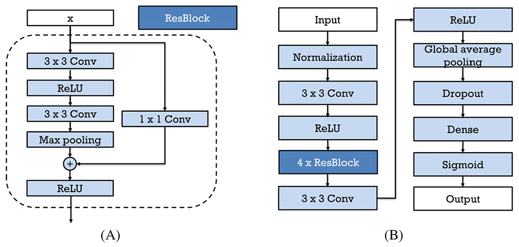
(A) ResBlock in the customized ResNet and (B) workflow of the customized ResNet

Figure 2(B) shows the structure of the ResNet used in this study. The input of the neural network is the 128 × 256 grayscale images, as described in the Image preprocessing session. The image is normalized before it goes through a 3 × 3 convolutional layer with a filter size 4 and a ReLU layer. And then, it passes four ResBlocks shown in (a) above. The filters of the convolutional layers in the four ResBlocks are 8, 16, 32, and 64, respectively. Then, the output passes through a 3 × 3 convolutional layer with 128 filters and a ReLU layer. After that, a global average pooling layer is used to generate a vector out of the feature maps, a dropout layer randomly sets input units to 0 with a frequency of 0.5 to help prevent overfitting, and a dense layer with the sigmoid activation function finally outputs a probability (a number between 0 and 1) that the input image belongs to the normal category. L2 regularization was applied to layer kernels in all convolutional layers and the dense layer. The network was trained for 200 epochs using the Adam solver¹⁷ with a batch size of 32 and a learning rate of 5e-5. The binary cross entropy loss, weighted according to the number of training images in each class, was used to deal with imbalanced dataset. Validation loss minimization was monitored for early stopping (with patience 20) to prevent overfitting. The learning rate was reduced by a factor of 0.2 of its previous value when the validation loss did not decrease for five epochs. The ResNet was implemented with Tensorflow. The training process takes about 9 hours on a Geforce GTX 2080 GPU, and the testing procedure takes <0.02 seconds for 8 ROIs, providing the potential for real-time diagnosis.

2.5 |. Image classification

After passing through the ResNet, each ROI was assigned a probability of being normal, referred to as a “score.” To enhance prediction stability, for each B-scan image, the average score of its ROIs was used to perform classification to predict if the entire B-scan image belonged to a normal or cancerous category. The area under receiver operating characteristic (ROC) curve (AUC) as well as sensitivity and specificity at the optimal point were calculated.

3 |. RESULTS AND DISCUSSION

In this section, the B scan and en face colorectal tissue images are presented. We utilize the designed ResNet to classify the B scan images, and analysis results are shown.

To better characterize the OCT imaging catheter, resolution is tested with a resolution target edge. The measured edge spread function (ESF) data along x and y directions are shown in Figure 3a and b marked with blue cross. The data are fitted with a cumulative distribution function (CDF) of normal distribution as depicted in red dashed lines. The resolution of the catheter is determined by the full width at half maximum (FWHM) of the derivatives of CDF, shown in green lines. The corresponding resolutions of this OCT catheter are around 6.5 um in x direction and 7.8 μm in y direction. Figure 3c shows the OCT catheter-depth wise cross-sectional B scan image of a section of layered Scotch™ tape. Around 20 layers can be discerned, corresponding to an imaging depth of ~1 mm.

FIGURE 3.

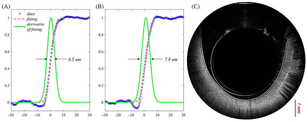
(A) Lateral resolution measurement of optical coherence tomography (OCT) catheter in the x direction (blue cross line: measured edge spread function (ESF) data; red dotted line: fitting curve with a normal distribution CDF; green solid line: derivative of the fitting CDF); (B) lateral resolution measurement in the y direction; and (C) depth-wise cross-sectional B scan image of a Scotch™ tape section wrapped around the catheter

Figure 4a shows a B-scan OCT of a rectum normal area, and Figure 4c depicts the rectum malignant tissue area with OCT endoscope images. Figure 4b and d are the corresponding H&E images. The benign region shows clear layers, while the malignant region shows a disordered structure. In Figure 4a, mucosa, muscularis mucosae, and submucosa layers can be discerned. Also, the benign region shows a dentate, or tooth-like structure, as described previously as a landmark in OCT images of normal human colorectal tissue, due to the increased optical transmissions through the normal crypt lumens.¹⁴

FIGURE 4.

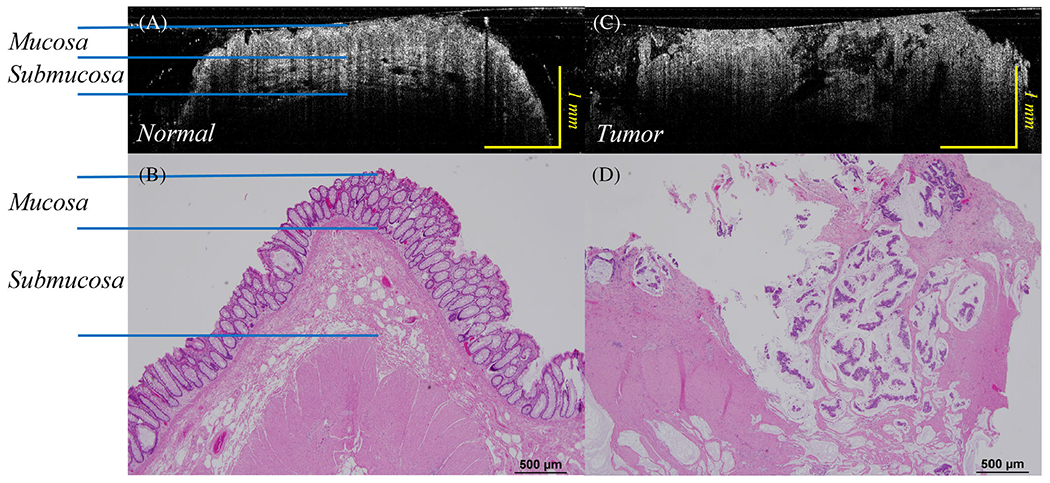
(A) B-scan optical coherence tomography (OCT) catheter image of normal rectum; (B) H&E image of corresponding normal rectal tissue; (C) B-scan OCT catheter image of a human rectal malignancy, while (D) displays a corresponding H&E image of the rectal tumor. Note the loss of regular, layered structure described by the normal images of the OCT scans from normal tissue

The en face images of a rectum sample are also shown here in Figure 5. The rectum sample image is shown in Figure 5a. Here, Figure 5b and c are acquired in the blue rectangular region and the red circular region in Figure 5a, respectively. Figure 5b depicts the en face OCT catheter image of normal rectum tissue area, and Figure 5c depicts the en face OCT catheter image of malignant rectum tissue area. A clear dotted pattern can be found in the benign rectum area shown in Figure 5b, while the rectal malignancy image shown in Figure 5c has a patchy and distorted structure. The dotted pattern can be attributed to the well-organized crypt pattern in normal colorectal tissue as shown in the corresponding H&E image Figure 5d. As colorectal cancer grows, it disrupts this well-organized pattern, and results in disordered, layer-less image patterns.

FIGURE 5.

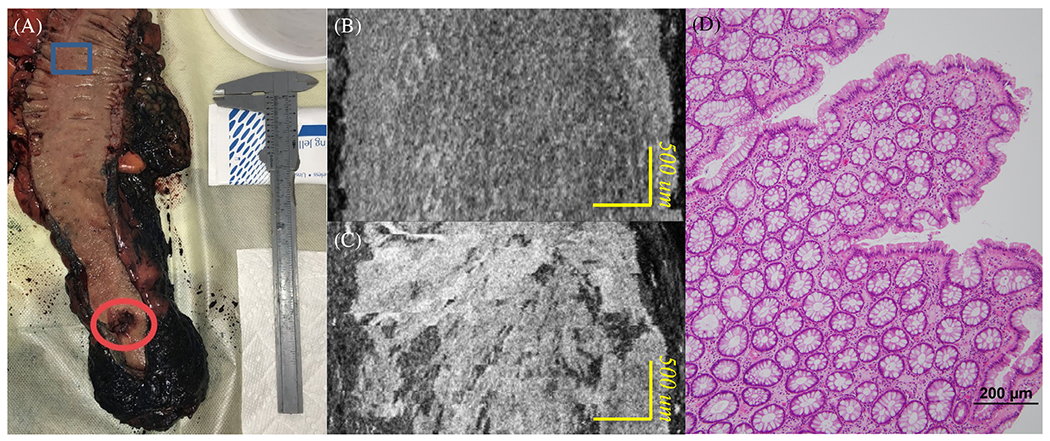
(A) Rectum sample; (B) en face OCT catheter image of a normal rectum tissue area; (C) en face OCT catheter image of a malignant rectum tissue area; and (D) en face H&E image of a normal rectum area

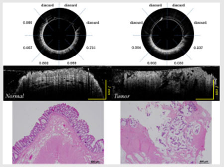
Figure 6 shows ResNet predictions for representative endoscopic images from (a) a normal region and (b) a cancerous region. The classifier gave high probabilities of being normal (>0.7) for all five ROIs in the normal region and low probabilities of being normal (<0.3) for the four ROIs in the cancerous region.

FIGURE 6.

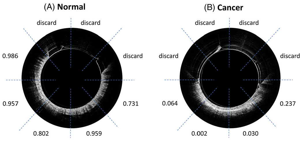
ResNet prediction of: (A) an optical coherence tomography (OCT) endoscope image of the normal region and (B) an OCT endoscope image of the cancerous region

Table 3 shows the average probabilities of no malignancy for thirteen testing areas acquired with the catheter. The classifier gave low probabilities (<0.5) to be normal for nine cancerous areas, and probabilities higher than 0.6 to be normal for all ten normal areas.

TABLE 3.

Testing results for catheter images from nine cancerous and ten normal areas

Case number, age, sex, tumor site	Number of B-scans	Predicted probability of normal (mean ± std)	Expected probability of normal	Pathologic results
T1, 52, m, rectum	214	0.4173 ± 0.0966	0	1.4 cm residual invasive adenocarcinoma, ypT3
T2, 52, f, rectum	292	0.2708 ± 0.2217	0	0.6 cm residual invasive adenocarcinoma, ypT3
T3, 44, m, rectum	235	0.4845 ± 0.1611	0	3 cm residual invasive adenocarcinoma, ypT3
T4, 86, f, colon	376	0.1754 ± 0.1550	0	5.5 cm invasive poorly differentiated adenocarcinoma of the cecum
T5, 72, m, rectum	400	0.3660 ± 0.1100	0	2.7 cm residual invasive adenocarcinoma, yPT2
T6, 60, f, rectum	318	0.2846 ± 0.1386	0	4.2 residual invasive rectal adenocarcinoma
T7, 73, m, rectum	698	0.3282 ± 0.1456	0	1.5 cm residual adenocarcinoma
T8, 67, m, rectum	390	0.4322 ± 0.1932	0	Moderately differentiated invasive adenocarcinoma, ypT2
T9, 71, f, rectum	376	0.3671 ± 0.1472	0	Moderately differentiated adenocarcinoma with invasion to muscular propria, ypT2
N1, 52, f, rectum	400	0.8770 ± 0.1110	1	Normal
N2, 44, m, rectum	400	0.8619 ± 0.0921	1	Normal
N3, 50, m, rectum	400	0.9233 ± 0.0412	1	Normal
N4, 86, f, colon	365	0.8039 ± 0.1093	1	Normal
N5, 72, m, rectum	379	0.6688 ± 0.1488	1	Normal
N6, 46, f, rectum	400	0.8159 ± 0.1168	1	Normal
N7, 60, f, rectum	390	0.8270 ± 0.0812	1	Normal
N8,73, m, rectum	395	0.8449 ± 0.1603	1	Normal
N9, 67, m, rectum	393	0.8508 ± 0.0911	1	Normal
N10, 71, f, rectum	387	0.9098 ± 0.0670	1	Normal

Figure 7 shows the ROC curve of the nine cancerous areas and ten normal areas. To balance the two classes, we picked 1890 B-scan images from cancer areas, with 210 images per area, and 1890 B-scan images from normal areas, with 189 images per area. The AUC is 0.975. If we pick 0.60 as a threshold for classification, then a sensitivity of 93.3% and a specificity of 92.6% can be achieved to classify a single B-scan image.

FIGURE 7.

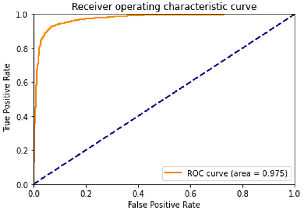
Receiver operating characteristic curve of nine cancerous and ten normal areas

There are several limitations to this study. Firstly, due to limited number of samples imaged with the catheter, the training data include both images from benchtop and catheter systems; however, the resolution and the ROI size of the benchtop and catheter are similar. Also, different areas have different numbers of ROIs, and images acquired in the same area have some level of similarities. Considering this, we split the dataset based on independent areas and balanced the ROI number in each area for the validation set. A larger catheter dataset will be acquired in the near future to validate the catheter system and the deep-learning model on in vivo colorectal cancer diagnosis. Secondly, this study is focused on diagnosis of colorectal cancer or residual cancer after treatment. However, OCT is not suitable to characterize treated tumor bed with no residual cancer due to extensive scar tissue. We have excluded three treated areas with no residual tumor, as the CNN model provides diagnosis close to those with cancer. Finally, this technology has not been evaluated with other colorectal pathologies. For example, the ability to differentiate adenomatous polyps from hyperplastic polyps is more clinically relevant. This task is planned for future in vivo studies.

4 |. SUMMARY

We describe the successful coupling of an OCT catheter designed for endoscopic application with a deep neural network to classify endoluminal OCT images as normal or malignant in real time. The fabricated probe has a lateral resolution of ~7 μm with an imaging depth of ~1 mm in tissue. By incorporating ResNet, our OCT system can achieve automated image classification and provide accurate diagnosis with AUC of 0.975 in real time.

Abbreviations:

AUC

the area under the ROC curve

CNN

convolutional neural network

GRIN

gradient refractive index

OCT

optical coherence tomography

ResNet

residual neural network

ROC

receiver operating characteristic

SMF

single-mode fiber

DATA AVAILABILITY STATEMENT

The data that support the findings of this study are available from the corresponding author upon reasonable request.

REFERENCES

- [1].Siegel RL, Miller KD, Fuchs HE, Jemal A, CA Cancer J. Clin 2021, 71(1), 7. 10.3322/caac.21654. [DOI] [PubMed] [Google Scholar]
- [2].Gora MJ, Quénéhervé L, Carruth RW, Lu W, Rosenberg M, Sauk JS, Fasano A, Lauwers GY, Nishioka NS, Tearney GJ, Gastrointest. Endosc 2018, 88(5), 830. 10.1016/j.gie.2018.07.009. [DOI] [PMC free article] [PubMed] [Google Scholar]
- [3].Gora MJ, Suter MJ, Tearney GJ, Li X, Biomed. Opt. Express 2017, 8(5), 2405. 10.1364/boe.8.002405. [DOI] [PMC free article] [PubMed] [Google Scholar]
- [4].Lee CS, Baughman DM, Lee AY, Ophthalmol. Retina 2017, 1(4), 322. [DOI] [PMC free article] [PubMed] [Google Scholar]
- [5].Gessert N, Heyder M, Latus S, Lutz M, Schlaefer A, arXiv 2018, 49(0), 1. 10.1007/s11548-018-1766-y. [DOI] [Google Scholar]
- [6].Abdolmanafi A, Duong L, Dahdah N, Adib IR, Cheriet F, Biomed. Opt. Express 2018, 9(10), 4936. 10.1364/boe.9.004936. [DOI] [PMC free article] [PubMed] [Google Scholar]
- [7].Urban G, Tripathi P, Alkayali T, Mittal M, Jalali F, Karnes W, Baldi P, Gastroenterology 2018, 155(4), 1069. 10.1053/j.gastro.2018.06.037. [DOI] [PMC free article] [PubMed] [Google Scholar]
- [8].Zhang R, Zheng Y, Mak TWC, Yu R, Wong SH, Lau JYW, Poon CCY, IEEE J. Biomed. Heal. Informatics 2017, 21(1), 41. 10.1109/JBHI.2016.2635662. [DOI] [PubMed] [Google Scholar]
- [9].Qi X, Sivak MV, Isenberg G, Willis JE, Rollins AM, J. Biomed. Opt 2006, 11(4), 044010. 10.1117/1.2337314. [DOI] [PubMed] [Google Scholar]
- [10].Hong J, Park BY, Park H, Proc. Annu. Int. Conf. IEEE Eng. Med. Biol. Soc. EMBS 2017, No. C, 2017, 2892. 10.1109/EMBC.2017.8037461. [DOI] [Google Scholar]
- [11].Zacharia R, Samarasena J, Luba D, Duh E, Dao T, James R, Ninh A, Karnes W, Am. J. Gastroenterol 2020, 115(1), 138. 10.14309/ajg.0000000000000429.Prediction. [DOI] [PMC free article] [PubMed] [Google Scholar]
- [12].Repici A, Badalamenti M, Maselli R, Correale L, Radaelli F, Rondonotti E, Ferrara E, Spadaccini M, Alkandari A, Fugazza A, Anderloni A, Galtieri PA, Pellegatta G, Carrara S, Di Leo M, Craviotto V, Lamonaca L, Lorenzetti R, Andrealli A, Antonelli G, Wallace M, Sharma P, Rosch T, Hassan C, Gastroenterology 2020, 159(2), 512. 10.1053/j.gastro.2020.04.062. [DOI] [PubMed] [Google Scholar]
- [13].Saratxaga CL, Bote J, Ortega-Morán JF, Picón A, Terradillos E, del Río NA, Andraka N, Garrote E, Conde OM, Appl. Sci 2021, 11(7), 1. 10.3390/app11073119. [DOI] [Google Scholar]
- [14].Zeng Y, Xu S, Chapman WC, Li S, Alipour Z, Abdelal H, Chatterjee D, Mutch M, Zhu Q, Theranostics 2020, 10(6), 2587. 10.7150/thno.40099. [DOI] [PMC free article] [PubMed] [Google Scholar]
- [15].Zeng Y, Nandy S, Rao B, Li S, Hagemann AR, Kuroki LK, McCourt C, Mutch DG, Powell MA, Hagemann IS, Zhu Q, J. Biophotonics 2019, 12(11), 1. 10.1002/jbio.201900115. [DOI] [PMC free article] [PubMed] [Google Scholar]
- [16].He K, Zhang X, Ren S, Sun J, Proc. IEEE Comput. Soc. Conf. Comput. Vis. Pattern Recognit 2016, 2016-Decem, 770. 10.1109/CVPR.2016.90. [DOI] [PMC free article] [PubMed] [Google Scholar]
- [17].Kingma DP; Ba Adam JL: A Method for Stochastic Optimization. 3rd Int. Conf. Learn. Represent. ICLR 2015 - Conf. Track Proc. 2015, 1–15. [Google Scholar]
Associated Data
This section collects any data citations, data availability statements, or supplementary materials included in this article.