Training Spiking Neural Networks in the Strong Coupling Regime

Abstract

Recurrent neural networks trained to perform complex tasks can provide insight into the dynamic mechanism that underlies computations performed by cortical circuits. However, due to a large number of unconstrained synaptic connections, the recurrent connectivity that emerges from network training may not be biologically plausible. Therefore, it remains unknown if and how biological neural circuits implement dynamic mechanisms proposed by the models. To narrow this gap, we developed a training scheme that, in addition to achieving learning goals, respects the structural and dynamic properties of a standard cortical circuit model: strongly coupled excitatory-inhibitory spiking neural networks. By preserving the strong mean excitatory and inhibitory coupling of initial networks, we found that most of trained synapses obeyed Dale’s law without additional constraints, exhibited large trial-to-trial spiking variability, and operated in inhibition-stabilized regime. We derived analytical estimates on how training and network parameters constrained the changes in mean synaptic strength during training. Our results demonstrate that training recurrent neural networks subject to strong coupling constraints can result in connectivity structure and dynamic regime relevant to cortical circuits.

1. Introduction

With recent advances in machine learning, recurrent neural networks are being applied to a wide range of problems in neuroscience as a tool for discovering dynamic mechanisms underlying biological neural circuits. The activity of network models trained either on tasks that animals perform or to directly generate neural activity has been shown to be consistent with neural recordings. Examples include context-dependent computation (Mante, Sussillo, Shenoy, & Newsome, 2013), neural responses in motor cortex (Sussillo, Churchland, Kaufman, & Shenoy, 2015), decision making with robust transient activities (Chaisangmongkon, Swaminathan, Freedman, & Wang, 2017), and flexible timing by temporal scaling (Wang et al., 2018). However, due to the large number of parameters, the network connectivities are often not constrained to be biologically plausible; thus, it remains unclear if and how biological neural circuits could implement the proposed dynamic mechanisms.

One approach for imposing biological constraints is to develop model architectures based on the detailed connectivity structure of the neural system. The complete connectome is available for certain invertebrates such as Drosophila, and it is possible to build recurrent neural network models constrained by the detailed structure of the connectome (Litwin-Kumar & Turaga, 2019; Eschbach et al., 2020; Zarin, Mark, Cardona, Litwin-Kumar, & Doe, 2019). In cortical regions of higher animals, however, obtaining a connectome and applying it for computational modeling purposes pose significant technical and conceptual challenges. Therefore, it is important to develop alternative methods for constraining the connectivity in a biologically plausible manner independent of the detailed connectome structure.

Recent studies have applied training methods to rate-based and spiking cortical circuits of excitatory and inhibitory neurons (Song, Yang, & Wang, 2016; Nicola & Clopath, 2017; DePasquale, Churchland, & Abbott, 2016; Kim, Li, & Sejnowski, 2019), but the focus was to preserve the excitatory-inhibitory structure (i.e., Dale’s law) without constraining the synaptic strength to a strong coupling regime (but see Ingrosso & Abbott, 2019, and Baker, Zhu, & Rosenbaum, 2019) that exhibits chaotic dynamics (Sompolinsky, Crisanti, & Sommers, 1988), asynchronous spiking (van Vreeswijk & Sompolinsky, 1996; Renart et al., 2010; Rosenbaum, Smith, Kohn, Rubin, & Doiron, 2017), spiking rate fluctuations (Ostojic, 2014), and inhibition stabilization (Tsodyks, Skaggs, Sejnowski, & McNaughton, 1997) as observed in neural recordings. Here, we show that by preserving the mean excitatory and inhibitory synaptic weights of a strongly coupled network, trained networks can exhibit large trial-to-trial variability in spiking activities, respect Dale’s law in most synapses without imposing strict constraints, and show a paradoxical phenomenon found in inhibition-stabilized networks. We provided analytical estimates on how the network and training parameters constrain the size of synaptic updates during network training. Our findings demonstrate that including synaptic constraints that maintain strong coupling strength allows spiking networks to respect dynamic properties of standard cortical circuit models in addition to achieving the learning goal.

2. Results

2.1. Learning under Excitatory and Inhibitory Synaptic Constraints.

The initial network consisted of an equal number of excitatory and inhibitory leaky integrate-and-fire neurons (N_E, N_I = 500) randomly connected with connection probability p = 0.1. The recurrent synaptic weights W_ij and the external inputs were sufficiently strong such that the total excitatory inputs to neurons (i.e., the sum of recurrent excitatory current and external input) exceeded spike threshold, and inhibitory feedback was necessary to prevent runaway excitation (see Figure 1A.i). In this parameter regime, neurons emitted spikes asynchronously and irregularly (see Figure 1A.ii) and had large trial-to-trial variability as measured by the Fano factor of spike counts in a 500 ms time window across trials starting at random initial conditions (see Figure 1A.iii). The synaptic connections to every neuron were statistically identical in that the presynaptic neurons were randomly selected, but the number of excitatory (pN_E) and inhibitory (pN_I) synaptic connections was fixed and their weights were constant depending only the the connections type, W_αβ, α,β ∈ {E, I} (i.e., fixed in-degree and constant weights). This network configuration resulted in a homogeneous firing-rate distribution (see Figure 1A.iv). Initial networks with nonidentical connectivity statistics that generate wide rate distributions were also investigated in section 2.6.

Figure 1:

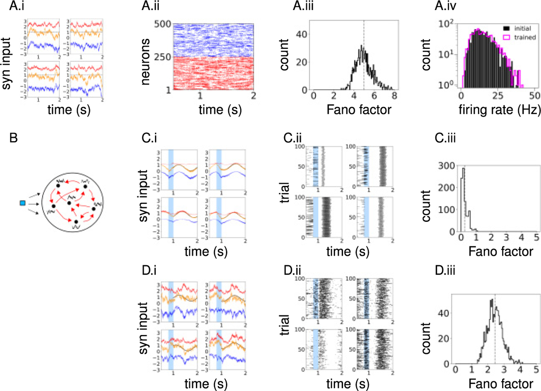
Comparison of FORCE- and ROWSUM-trained network activities. (A) Population activity of the initial network. (A.i) Synaptic inputs to example neurons; excitatory (red), inhibitory (blue), and total (orange) inputs; external input is added to the excitatory and total inputs; dashed line indicates the spike threshold. (A.ii) Spike raster of sample neurons. (A.iii) Fano factor of all neurons; spike counts across trials in a 500 ms time window are used to compute the Fano factor and averaged over the training window to obtain a time-averaged Fano factor for each neuron. (A.iv) Firing-rate distribution of neurons; initial network (black), ROWSUM-trained network (magenta). (B) Schematic of network training. Brief external input (blue) is applied to trigger learned response; individual neurons learn their own target patterns (black); recurrent synaptic connections (red) are modified to generate the target patterns. (C) Population activity of a FORCE-trained network. (C.i) Synaptic inputs to example neurons. (C.ii) Spike trains of the same neurons in panel C.i across trials starting at random initial conditions. (C.iii) Fano factor of trained neurons. (D) Population activity of a ROWSUM-trained network; same color codes as in panel C.

In the present study, spiking neural networks were trained to generate desired recurrent activity patterns. In related work, Rajan, Harvey, and Tank (2016) trained a recurrent rate network to generate sequential activity observed in the posterior parietal cortex in mice, Laje and Buonomano (2013) stabilized inherent chaotic trajectories of the initial rate network, and Kim and Chow (2018) generated arbitrarily complex activity patterns in recurrent spiking networks. We point out that these tasks are different from the standard machine learning tasks, such as image classification, in that individual neurons within the network learn to generate certain activity patterns. Other studies have investigated performing machine learning tasks in spiking networks (Nicola & Clopath, 2017; Huh & Sejnowski, 2018).

Specifically, our goal was to train the synaptic current u_i(t) to each neuron i = 1,…, N such that it followed target activity pattern f_i(t) defined on time interval t ∈ [0, T]. To trigger the target response, each neuron was stimulated by a constant input with random amplitude for 200 ms (see Figure 1B). We treated every neuron’s synaptic current as a read-out, which made our task equivalent to training N recurrently connected read-outs. For spiking network models with current-based synapses, neuron i’s synaptic current u_i can be expressed in terms of the spiking activities of other neurons r_j, j = 1,…, N through the exact relationship $u_i={\sum }_j{W}_{ij}{r}_j$ (see equations 4.1 and 4.4 for details). Therefore, we adjusted the incoming synaptic connections W_ij, j = 1,…, N to neuron i by the recursive least squares algorithm (Haykin, 1996) in order to generate the target activity. This training scheme allowed us to set up independent objective functions for each neuron and potentially update them in parallel.

The objective function included the error between the synaptic currents and target patterns, and, importantly, we considered two types of synaptic regularization The first type regularized the standard L₂-norm of the incoming synaptic weights to each neuron i,

$$C_{FORCE}^i={\int }_0^T{\left(f_i\left(t\right)-u_i\left(t\right)\right)}^{2}dt+\lambda \sum _j{W}_{ij}^2,$$ (2.1)

and $C_{FORCE}={\sum }_{i=\mathbf{1}}^N{C}_{FORCE}^i$ was the full objective function. The second type regularized the sums of excitatory and inhibitory synaptic weights, respectively, to each neuron i, in addition to the L₂-norm,

$$C_{ROWSUM}^i={\int }_0^T{\left(f_i\left(t\right)-u_i\left(t\right)\right)}^{2}dt+\lambda \sum _j{W}_{ij}^2+\mu \sum _{\alpha \in \left\{E,I\right\}}{\left(\sum _{j\in \alpha }{W}_{ij}\right)}^2,$$ (2.2)

and $C_{ROWSUM}={\sum }_{i=\mathbf{1}}^N{C}_{ROWSUM}^i$ was the full objective function. The first type, which is equivalent to the algorithm of Sussillo and Abbott (2009) and used previously in spiking networks (Kim & Chow, 2018; Nicola & Clopath, 2017), will be referred to as FORCE training. The second type will be referred to as ROWSUM training since it regularizes the sum of excitatory and inhibitory weights, respectively, in each row of the connectivity matrix.

We note how the hyperparameters λ and μ can be interpreted. At first glance, it appears that large, positive values of λ and μ should reduce the magnitude of synaptic weights in trained networks. However, the recursive least squares is different from the standard gradient descent algorithms in that the synaptic update rule is not derived from the gradient of cost function. Instead, it finds a critical point to the difference of gradients of cost function at two consecutive time points (see section 4.2). This implies that large, positive values of λ and μ penalize the size of synaptic updates, resulting in small synaptic updates or slow learning rate (see Sussillo & Abbott, 2009, for further discussion). Therefore, the synaptic weights trained with large λ and μ stay close to their initial weights if trained by the recursive least squares algorithm.

We first considered simple target patterns consisting of sinusoidal waves $f_i\left(t\right)=A\sin \left(2\pi t/T+{\varphi }_i\right)+{\overline{u}}_i$ defined on t ∈ [0, T] with duration T = 1000 ms, random phase ϕ_i, fixed amplitude A, and bias ${\overline{u}}_i$. The amplitude A was the standard deviation of synaptic currents in time averaged over all neurons, and the bias ${\overline{u}}_i$ for neuron i was the mean synaptic current to neuron i in the initial network. After adjusting the recurrent weights with two training schemes, we examined the differences in trained network activities. Notably, the large fluctuations of excitatory and inhibitory synaptic currents in the initial network were not observed in FORCE-trained networks. Instead, the total synaptic currents closely followed the target patterns with little error (see Figure 1C.i). Such synaptic currents led to highly regular spikes with little variability across trials starting at random initial conditions (see Figure 1C.ii), resulting in a small Fano factor (see Figure 1C.iii). In contrast, ROWSUM-trained networks, which were encouraged to preserve the initial excitatory and inhibitory synaptic weights, exhibited strong synaptic fluctuations, irregular spike trains, and large trial-to-trial variability (see Figure 1D.i,ii,iii). Also, the firing-rate distribution of trained neurons closely followed the firing-rate distribution of untrained neurons, showing that sinusoidal targets minimally altered the firing-rate distribution (see Figure 1A.iv).

2.2. ROWSUM Constraint Can Preserve the Mean Excitatory and Inhibitory Synaptic Strength.

We examined the trained synaptic weights to better understand the underlying network structure that led to different levels of variability in neuron activities in the FORCE- and ROWSUM-trained networks. We found that the excitatory and inhibitory synaptic weights of the initial network were both redistributed around zero by the FORCE learning (see Figure 2A.i), and the fraction of synapses that violated Dale’s law increased gradually as the number of training iteration increased (see Figure 2A.ii). The mean strength of excitatory and inhibitory synaptic connections to each neuron also moved toward zero (see Figure 2A.iii). This shift in synaptic weight distributions can be explained by the L₂-regularization term in equation 2.1 that allowed small synaptic weights, and, as a consequence, the mean excitatory and inhibitory synaptic connections to each neuron were significantly smaller than those of the initial network. After removing synaptic connections that violated Dale’s law, the FORCE-trained network was able to generate the target patterns with high accuracy (see Figure 2A.iv). These findings suggested that the network connectivity resulting from FORCE training was degenerating and highly tuned to produce the target dynamics with minimal error.

Figure 2:

Network connectivity of trained networks. (A) FORCE-trained network. (A.i) Distribution of synaptic weights of the FORCE-trained network (120 training iterations); red (blue) shows synapses that are excitatory (inhibitory) in the initial network; dotted line shows the initial synaptic strength. (A.ii) Fraction of excitatory (red) and inhibitory (blue) synapses that violate Dale’s law after each training iteration. (A.iii) Mean strength of synaptic connections to individual neurons after FORCE training; orange (green) dots show connections that are excitatory (inhibitory) in the initial network; black dots show the initial mean synaptic weights. Mean excitatory and inhibitory weights to neurons were identical in the initial network since in-degrees were fixed and synaptic weights were constant. (A.iv) Performance of trained networks, measured as the correlation between target patterns and synaptic activities, when synapses violating Dale’s law are removed; fraction of clipped synapses equals one if all synapses violating Dale’s are removed. (B) Same as in panel A, but for a ROWSUM-trained network with fixed in-degree and constant weights. (C) Same as in panel A, but for a ROWSUM-trained network with random indegrees and gaussian weights; correction terms are added to reconcile differences in synaptic weights each neuron receives.

For the ROWSUM training, we used the same network and training parameters as the FORCE training but included the additional penalty that constrained the sums of excitatory and inhibitory synaptic weights, respectively, to each neuron. We found that the excitatory and inhibitory weights of the trained synapses were distributed around their initial values (see Figure 2B.i), and the fraction synapses that violated Dale’s law increased in the early stage of training but gradually decreased and stabilized as the training continued (see Figure 2B.ii). The mean strength of excitatory and inhibitory synaptic connections to each neuron after training deviated little from the initial mean synaptic weights (see Figure 2B.iii), demonstrating that the ROWSUM regularization allowed the trained network to preserve the mean excitatory and inhibitory strength of the strongly coupled initial network. The fraction of synapses that violated Dale’s law after training (approximately 5% and 2% of excitatory and inhibitory connections, respectively) was significantly smaller than a FORCE-trained network (40% and 20%, respectively), and removing them had only a small impact on the network performance (see Figure 2B.iv).

Next, we investigated if ROWSUM training was applicable to initial networks with random in-degrees and weights. To this end, we constructed an Erdos-Renyi graph where each synaptic connection was generated independently with probability p, that is, Pr(W_ij ) = p, if neuron j connects to neuron i, resulting in a connectivity matrix with a nonconstant in-degree distribution. The synaptic weight of each connection was sampled from gaussian distribution with mean W_αβ and standard deviation W_αβ/5 for α, β ∈ {E, I} to ensure the initial network respected Dale’s law. In order to reconcile differences in synaptic weights neurons received, we added a correction term to nonzero elements in each row of the connectivity matrix such that the sum of excitatory and inhibitory synaptic weights to neuron i ∈ α was equal to pN_Ew_αE and pN_Iw_αI, respectively. Including such correction terms resulted in a homogeneous rate distribution, as opposed to a wide rate distribution, and trained networks qualitatively agreed with those initialized with fixed indegrees and constant weights (see Figure 2C.i–iv).

These findings demonstrated that constraining the sums of excitatory and inhibitory synaptic weights, respectively, allowed the individual synapses to learn target patterns while keeping the mean synaptic strength close to the initial values. Since the excitatory and inhibitory synaptic weights of the initial network were strong enough to generate variable spiking activity, the trained network was able to inherit the dynamic property of the initial network.

Before turning to limitations of training complex target patterns and initial networks without the correction terms in sections 2.4 and 2.6 we examined if other aspects of the initial network dynamics were inherited by the trained network when the mean excitatory and inhibitory synaptic weights were preserved.

2.3. ROWSUM Constrained Networks Inherit Dynamic Features of Inhibition-Stabilized Network.

The initial network was set up to be an inhibition-stabilized network (ISN), where strong recurrent excitatory connections were stabilized by inhibitory feedback without which the network would exhibit runaway excitation (Tsodyks et al., 1997; Sanzeni et al., 2019; Sadeh & Clopath, 2020). An ISN exhibits a paradoxical phenomenon where an external stimulus that excites inhibitory neurons decreases their firing rates. Although the stimulus can transiently increase the firing rates of inhibitory neurons, this activity inhibits excitatory neurons that in turn reduce recurrent excitatory input to inhibitory neurons. The reduction in recurrent excitation is larger than the external stimulus, resulting in a net decrease in excitatory input to inhibitory neurons. Such large reduction in recurrent excitation occurs because strongly connected excitatory neurons respond to changes in input with large gain (Tsodyks et al., 1997; Sanzeni et al., 2019; Sadeh & Clopath, 2020).

To verify that the initial network operated in the inhibition-stabilized regime, we injected additional excitatory stimulus to inhibitory neurons (see Figure 3A) and found that both excitatory and inhibitory population firing rates decreased (see the shaded region in Figure 3B.i). As the external stimulus to inhibitory neurons was further increased, the excitatory population rate decreased gradually, and once the excitatory population activity was fully suppressed, the firing rate of inhibitory neurons started increasing with the external stimulus (see Figure 3B.ii). These dynamic features are consistent with a theoretical analysis of ISNs that the paradoxical phenomenon occurs only within a limited range of stimulus intensity. In a strong stimulus regime, the network is effectively reduced to a single inhibitory population: therefore, the paradoxical phenomenon can no longer exist.

Figure 3:

ROWSUM-trained networks exhibit dynamic features of inhibition-stabilization. The shaded region shows the time period during which inhibitory neurons are excited by additional external stimulus. (A) Schematic of network structure where inhibitory neurons are stimulated. (B) Initial network activities in response to stimulating inhibitory neurons. (B.i) Excitatory (red) and inhibitory (blue) population firing rates with (dotted) and without (solid) the additional stimulus to inhibitory neurons. (B.ii) Population firing rates as a function of stimulus intensity. (B.iii) Trial-averaged firing rates of individual neurons without stimulus versus changes in neurons, firing rates due to the stimulus. (C) Synaptic inputs to individual neurons. (C.i) Distribution of changes in time-averaged synaptic inputs to individual neurons due to the stimulus. For excitatory (inhibitory) inputs, negative (positive) value implies reduction in the average input; excitatory (red), inhibitory (blue), and total (orange). (C.ii) Synaptic inputs to a neuron in an unstimulated network are compared to those in a stimulated network (green). (D) Changes in total synaptic input versus changes in the number of emitted spikes due to the stimulus; dots show individual neurons. (E) The number of emitted spikes in an unstimulated network versus changes in the number of emitted spikes due to the stimulus; dots show individual neurons. (F) Trial-averaged firing rate of sample neurons with (dotted) and without (solid) the stimulus. (G) Same as in panel B but for a ROWSUM-trained network. (H) Same as in panel B but for a FORCE-trained network.

To better understand how individual neurons responded to the external stimulus, we stimulated inhibitory neurons over multiple trials and examined the trial-averaged firing rates of individual neurons with and without the stimulus. The relationship between the trial-averaged firing rate of unstimulated neurons and changes in their firing rates due to the stimulus revealed that neurons with high baseline firing rates resulted in a large reduction in their spiking activities (see Figure 3B.iii).

Since the ROWSUM training preserved the mean synaptic strength of the initial network, we investigated if, in addition to learning target activity patterns, the trained network preserved unique features of the initial network’s population dynamics characterized by strong excitation and feedback inhibition. To test if the ROWSUM-trained network exhibited the dynamic features of ISN, we evoked the learned activity patterns in the trained network and then injected an external stimulus that excited all inhibitory neurons during the second half of the target patterns. We found that although the temporal average of recurrent excitatory and inhibitory inputs to individual neurons were both reduced in their magnitudes due to the stimulus (see Figure 4Ci, red and blue), the distribution of total synaptic inputs to neurons was centered around zero and did not exhibit apparent hyperpolarizing effects at the population level (see Figure 4Ci, orange). When we examined single trial responses with and without the stimulus, neurons whose total synaptic inputs were hyperpolarized by the stimulus (negative side of the orange curve in Figure 4C.i) had a large reduction in their spiking activities (negative side in Figure 4D) in comparison to the increased spiking activities (positive side in Figure 4D) in other neurons whose total synaptic inputs were depolarized by the stimulus (positive side of the orange curve in Figure 4C.i). As a result, the population firing rate decreased by 5 Hz (see the red line in Figure 4D) consistently with the firing-rate reduction seen in the stimulated initial network (see Figure 4B.i). In addition, neurons with a high spiking rate in the unstimulated network had a large reduction in their emitted spikes (see Figure 3E) in agreement with the trial-averaged response in the initial network (see Figure 3B.iii).

Figure 4:

Learning complex activity patterns under the ROWSUM constraint on excitatory and inhibitory synapses. Target patterns consist of trajectories generated from the Ornstein-Ulenbeck process. (A) Synaptic inputs to trained neurons; excitatory (red), inhibitory (blue), and the total (orange) inputs; external input is added to the excitatory and total inputs. (B) Spike trains of the same neurons in panel A across trials. (C) Fano factor of trained neurons; dashed line indicates the mean. (D) Distribution of neurons firing rates during the trained time window. (E) Mean strength of trained synaptic weights to each neuron; orange (green) dots show the mean strength of synaptic weights that are excitatory (inhibitory) prior to training; black dots show the mean strength of initial excitatory (positive) and inhibitory (negative) synaptic weights. (F) Fraction of excitatory (red) and inhibitory (blue) synapses that violate Dale’s law after each training iteration. (G) Distribution of trained synaptic weights; red (blue) shows synapses that are excitatory (inhibitory) in the initial network; dotted line shows the initial synaptic strength. (H) Distribution of trained synaptic weights; all the synapses (black); outgoing synapses from top (green) and bottom (purple) 40% of neurons ordered by their firing rates.

The effects of exciting inhibitory neurons were observed more clearly in trial-averaged firing rates in individual neurons and population rates. Without additional stimulus to inhibitory neurons, the trial-averaged firing rates followed the target rate patterns as trained (see Figure 3F). However, when the external stimulus was injected to excite the inhibitory neurons, their firing rates decreased compared to those of unstimulated neurons, and similar effects were observed in both the excitatory and inhibitory population firing rates (see Figure 3G.i). We also found that the paradoxical effect was observed in a limited stimulus range for the ROWSUM-trained network (see Figure 3G.ii), and the neurons with high trial-averaged firing rates in an unstimulated network had a larger reduction in their spiking activities due to the stimulus (see Figure 3G.iii). These findings show that the ROWSUM-trained network inherited the dynamic features of the initial network.

To test if the FORCE-trained network exhibited similar dynamic features, we trained an inhibition-stabilized network without the ROWSUM regularization term. Injecting excitatory inputs to inhibitory neurons in the FORCE-trained network did not elicit a paradoxical effect: the inhibitory population rate increased, and the excitatory population rate decreased (see Figure 3H.i). Moreover, the paradoxical effect was not observed over a wide range of stimulus intensity (see Figure 3H.ii). Also, a large number of neurons increased their trial-averaged firing rates due to the stimulus (see Figure 3H.iii). These findings suggest that the FORCE-trained network did not operate in the inhibition-stabilized regime.

2.4. Limitations of Constraining Excitatory and Inhibitory Synaptic Weights.

So far, (1) the initial network connectivity was adjusted such that the sum of excitatory and inhibitory synaptic weights to neurons was uniform, and (2) the target patterns were simple sinusoidal perturbations of the initial synaptic activities. These initial network setup and target patterns led to a relatively homogeneous firing-rate distribution. We asked if the ROWSUM training was still effective when either the initial network connectivity or the set of target patterns was no longer fine-tuned. To this end, we investigated if both the initial network setup and the choice of target functions can limit the effectiveness of ROWSUM training. In this section, we consider initial networks whose total excitatory and inhibitory synaptic weights across neurons were uniform as before, but neurons were trained on complex target patterns to encourage a wide range of activity patterns. Initial networks with nonidentical synaptic weights across neurons are discussed in section 2.6.

To generate complex target patterns, we sampled trajectories from the Ornstein-Ulenbeck process with decay time constant 200 ms and applied the moving average with a 100 ms time window to smooth out fast fluctuations. The amplitude of trajectories was scaled so that their standard deviation matched with that of synaptic currents of the initial network. Each neuron was trained on independently generated trajectories with the ROWSUM constraints on the sum of excitatory and inhibitory synaptic weights, respectively. We found that although the trained neurons successfully tracked the complex trajectory patterns (see Figure 4A), the trial-to-trial variability was relatively low (see Figures 4B and 4C), and the firing-rate distribution was wide, including many low-firing-rate neurons (see Figure 4D).

Examining the trained weights showed that the mean strength of excitatory and inhibitory synaptic connections to each neuron did not deviate from their initial values, showing that the ROWSUM constraints worked effectively (see Figure 4E). However, the fraction of synapses that violated Dale’s law increased gradually with training iterations (see Figure 4F), and the distribution of synaptic weights of the trained network showed that a large number of synapses were degenerating (see Figure 4G). In particular, the synapses outgoing from neurons with high firing-rate were concentrated near zero, in contrast to those from neurons with low firing rates (see Figure 4H).

To better understand how the trained synaptic weights might depend on the firing-rate distribution of presynaptic neurons, we analytically estimated the size of synaptic weight updates assuming presynaptic neurons followed simplified rate distributions (see section 4.4 for details). The analytical expressions suggested that for a homogeneous rate distribution (i.e., all neurons have the same rate), the size of synaptic update is small, O(1/(μK)), due to the cancellation effect by the ROWSUM regularization (see equation 4.21). On the other hand, for an inhomogeneous rate distribution consisting of high- and low-firing-rate neurons, the size of the synaptic update is large, O(1), and the synaptic connections from two neuron types are updated in opposite directions (see equation 4.22). The analytical results from the inhomogeneous rate distribution were consistent with the full ROWSUM training in that the synapses from high-firing-rate neurons concentrated near zero, while those from low-firing-rate neurons had a wide distribution, including strong synapses (see Figure 4H). Moreover, analysis of the homogeneous rate distribution suggested that applying the ROWSUM constraints to subpopulations that share similar activity levels can reduce deviations of individual synaptic weights from their mean values.

2.5. ROWSUM Constraints on Multiple Subpopulations.

In order to overcome the limitations of applying ROWSUM constraints to a population of neurons with a wide firing-rate distribution, we further divided the neurons into multiple subpopulations where neurons within a subpopulatioin shared similar levels of spiking activities. First, to estimate an individual neuron’s firing rate after training, external inputs that followed the target patterns were injected into each neuron. Then the excitatory and inhibitory neurons were respectively ordered by their time-averaged firing rates and divided into M subpopulations of equal sizes by assigning the αth N_E/M excitatory and N_I/M inhibitory neurons to E_α and I_α, respectively. Finally, the ROWSUM constraint was applied to synapses from each subpopulation E_α, I_α, α = 1,…, M, separately, resulting in the following synaptic constraint for training neuron i:

$$\sum _{\alpha =\mathbf{1}}^M\left[{\left(\sum _{j\in E_{\alpha }}{W}_{ij}\right)}^2+{\left(\sum _{j\in I_{\alpha }}{W}_{ij}\right)}^2\right].$$ (2.3)

See Figure 5A for a schematic of constraining multiple subpopulations.

Figure 5:

Learning complex activity patterns under the ROWSUM constraint on multiple subpopulations. Target patterns consist of trajectories generated from the Ornstein-Ulenbeck process. (A) Schematic of constraining multiple subpopulations; black dot indicates one neuron; transparency indicates the within-group firing rate. (B) Excitatory (red), inhibitory (blue), and total (orange) synaptic inputs to trained neurons. (C) Spike trains of the same neurons in panel A across multiple trials. (D) Fano factor of trained neurons; dashed line indicates the mean. (E–G) Excitatory and inhibitory neurons are ordered by firing rates and assigned to five subpopulations (i.e., 100 neurons in each group); low- to high-rate groups are shown from left to right; neurons in the αth excitatory and inhibitory subpopulations are shown in the same panel, group α. (E) Distribution of firing rates of neurons in group α; the within-group average firing rates shown. (F) Mean strength of synaptic connections that each neuron in the αth excitatory (orange) and inhibitory (green) subpopulations receive from other neurons in the same subpopulation; black dots show the mean strength of initial connections. (G) Synaptic weight distribution of outgoing connections from neurons in the αth excitatory (red) and inhibitory (blue) subpopulations. The percentage of synapses (with respect to the total number of synapses in the network) that violates Dale’s law by the neurons in each group are shown. (H) Fraction of excitatory (red) and inhibitory (blue) synapses that violates Dale’s law after each training iteration; each line represents outgoing synapses from neurons in the αth subpopulation; light to dark color shows subpopulation 1 to 5. (I) Distribution of trained synaptic weights (black); outgoing synapses from top (green) and bottom (purple) 40% of neurons ordered by firing rates; dashed lines indicate initial synaptic weights. (J) Performance of trained networks after removing synapses that violate Dale’s law; constraints on multiple (black) and excitatory-inhibitory (orange) populations.

Overall, we found that the synaptic fluctuations (see Figure 5B) and trial-to-trial spiking variability (see Figures 5C and 5D; average Fano factor 1.5) increased when multiple subpopulations were constrained, in contrast to the network constrained by the excitatory and inhibitory connections only (see Figures 4B and 4C).

Next, we combined the αth excitatory and inhibitory subpopulations into one group and examined their features. The within-group average firing rates increased sequentially in agreement with how neurons were assigned to each group (see Figure 5E; αth excitatory and inhibitory groups shown in the same panel). The mean strength of synaptic connections from low-rate neurons showed little deviation from their initial mean values (see Figure 5F, group 1), while synaptic connections from high-rate neurons (group 5) showed larger deviations. As will be further analyzed in section 2.7, the firing rates of presynaptic neurons and the inverse of the number synapses constrained under the ROWSUM regularization are among the factors that determine how much a recursive least squares algorithm can change the mean synaptic weights. In light of this analysis, the high firing rates and the reduced number of neurons in a subpopulation provide an explanation of why the mean synaptic weights from neurons in high-rate groups deviated from the initial mean weights.

Importantly, the fraction of synapses that violated Dale’s law was reduced (8%; see Figures 5G and 5H) compared to that found in the network trained under constrained excitatory and inhibitory connections (14%; see Figure 4F). Also, the distribution of synaptic weights from the low- and high-firing-rate neurons no longer exhibited drastic differences (see Figure 5I). Interestingly, the fraction of synapses that violated Dale’s law was smaller in groups consisting of high-firing-rate neurons (see the percentages shown in Figure 5G). Tracking the synapses that violated Dale’s law during training revealed that although such synapses increased rapidly during the early phase of training, they diminished quickly and stabilized to lower values, particularly in the high-firing-rate groups (see Figure 5H). Moreover, removing the synapses that violated Dale’s law did not significantly affect the performance in networks trained under multiple subpopulation constraints; however, a network trained under the excitatory and inhibitory constraints suffered from reduced performance (see Figure 5J).

2.6. Training Initial Networks with Random Connectivity.

In this section, we turn to initial networks for which the sums of excitatory and inhibitory synaptic weights to each neuron, respectively, are no longer identical across neurons. We constructed an Erdos-Renyi graph with connection probability p, which resulted in a nonconstant in-degree distribution and assigned constant weights to each connection type W_αβ for α, β ∈ {E, I}. To revive the inactive neurons present in such a network, we selected the bottom half of the neurons from their mean synaptic weight distribution and added a correction term to the incoming synaptic weights such that the sum matched the expected value pN_βW_αβ (see section 4.1 for details). The resulting network exhibited a wide firing-rate distribution, including many low-firing-rate neurons (see Figure 6A.i) and large trial-to-trial spiking variability (see Figures 6A.ii and 6A.iii).

Figure 6:

Training initial networks with random connectivity. Synaptic weights to neurons in the bottom half of the mean synaptic weight distribution are corrected to their expected values pN_βW_αβ . Target patterns consist of sinusoidal waves with random phases and fixed amplitude. (A) Population activity of an initial network. (A.i) Distribution of neurons’ firing rates. (A.ii) Distribution of neurons’ Fano factor. (A.iii) Spike raster of sample neurons. (B) Network trained with the ROWSUM constraint on excitatory and inhibitory synapses. (B.i) Fraction of synapses that violates Dale’s law after each training iteration. (B.ii) Fano factor of trained neurons. (B.iii) Synaptic weight distribution of a trained network (black); Outgoing synapses from top 40% of neurons ordered by firing rates (green). (C) Same as in panel B but for a network trained with the ROWSUM constraint on multiple subpopulations.

To avoid compounding the effects of network initialization and target choices, we chose sinusoidal functions as the target patterns since they minimally altered the initial firing-rate distribution. Then we trained the initial network with two different ROWSUM constraints developed in sections 2.4 and 2.5.

First, when only the excitatory and inhibitory synaptic connections to neurons were constrained, the fraction of synapses that violated Dale’s law increased with training iterations (see Figure 6B.i) and the spiking activities of the trained network were highly regular across trials (see Figure 6B.ii). We found that, similar to networks trained to learn complex target patterns (see Figure 4H), the synaptic connections from high-firing-rate neurons were degenerating (see Figure 6B.iii).

On the other hand, when the ROWSUM constraint was applied to multiple excitatory and inhibitory subpopulations as discussed in section 2.5 (i.e., five subpopulations for the excitatory and inhibitory neurons, respectively), the fraction of synapses violating Dale’s law remained low (see Figure 6C.i), and the spiking variability was relatively large, with the mean Fano factor close to 1.5 (see Figure 6C.ii). Moreover, the synaptic weight distribution, particularly the synaptic connections from high-rate neurons, did not converge toward zero (see Figure 6C.iii). These training results demonstrated that applying the ROWSUM constraint on multiple subpopulations can be an effective training scheme even when the the initial network included random connectivity that generated a wide firing-rate distribution.

2.7. Analytical Upper Bound on Synaptic Weight Updates.

Since retaining the strong coupling strength of the initial network was critical for generating large synaptic fluctuations and inhibition-dominant dynamics, we inquired how the ROWSUM training was able to tightly constrain the mean synaptic weights such that the mean excitatory and inhibitory synaptic weights to each neuron stayed close to their initial values (Figures 2B, 2C, 2E, and 2F). In particular, we sought to derive an analytical upper bound on the changes in the sums of excitatory and inhibitory synaptic weights, respectively, in terms of the network and training parameters.

For the analysis, we considered a vector of synaptic connections w to an arbitrary neuron i in the network whose weights were modified by the recursive least squares (RLS) algorithm under the ROWSUM regularization. Elements of w are denoted by w_j = W_ij for j = 1,…, K, where K is the total number of synapses modified under ROWSUM regularization. Then the sums of excitatory and inhibitory synaptic weights are defined, respectively, by

$$z_{\alpha }=\mathbf{w}\cdot {\mathbf{1}}_{\alpha }\hspace{1em}\text{for}\hspace{1em}\alpha =E,I.$$ (2.4)

Here, 1_E denotes a vector (1,…, 1, 0,…, 0) where the number of 1’s is equal to the number of excitatory synapses K_E modified under ROWSUM regularization and the rest of K_I = K – K_E elements is 0. 1_I = (0,…, 0, 1,…, 1) is defined similarly for the inhibitory synapses modified under the ROWSUM regularization.

From the RLS algorithm (see equation 4.9), the changes in the sums of excitatory and inhibitory synaptic weights at each synaptic update obey

$$\delta z_{\alpha }^n=z_{\alpha }^n-z_{\alpha }^{n-\mathbf{1}}=e^n{\mathbf{\sigma }}_{\alpha }^n\cdot {\mathbf{r}}^n\hspace{1em}\text{for}\hspace{1em}\alpha =E,I,$$ (2.5)

where

$${\mathbf{\sigma }}_{\alpha }^n=P^n{\text{1}}_{\alpha }$$ (2.6)

and

$$P^n={\left[\sum _{t=\mathbf{1}}^n{\mathbf{r}}^t{\left({\mathbf{r}}^t\right)}^{\prime }+\lambda I+\mu {\mathbf{1}}_E{\mathbf{1}}_E^{\text{'}}+\mu {\mathbf{1}}_I{\mathbf{1}}_I^{\text{'}}\right]}^{-\mathbf{1}}.$$ (2.7)

Since ${\mathbf{\sigma }}_{\alpha }^n$ was the only term in the synaptic update rule (see equation 2.5) that depended on training and network parameters, it constrained the upper bound on synaptic weight changes. In simulations, the elements of ${\mathbf{\sigma }}_{\alpha }^n$ fluctuated in the early phase of training but stabilized as the training iteration n increased (see Figure 7A). Based on this observation, we derived an approximation of ${\mathbf{\sigma }}_{\alpha }^n$ for large n and obtained an estimate on its upper bound.

Figure 7:

Analytical upper bound on synaptic updates. (A) Elements in ${\mathbf{\sigma }}_{\alpha }^n$ stabilize if the training iteration d becomes large. ${\mathbf{\sigma }}_{\alpha }^n$ of sample neurons are shown; excitatory (red) and inhibitory (blue). ${\sigma }_{\alpha }^0={\left(\lambda +\mu K_{\alpha }\right)}^{-1}$ denotes the initial value. (B) Comparison of the actual ${\mathbf{\sigma }}_{\alpha }^n$ and the theoretical estimate ${\widehat{\mathbf{\sigma }}}_{\alpha }^d$ as a function of training iteration d; actual (solid), theory (dotted), and difference of actual and theoretical (red). (C) Comparison of the actual values ${\mathbf{\sigma }}_{\alpha }^n$ and the theoretical estimates ${\widehat{\mathbf{\sigma }}}_{\alpha }^d$ at training iteration d = 120. Scatter plot shows the vector elements of all neurons; identity line (gray). (D) Total changes in the mean synaptic weights $\text{Δ}\overline{\mathbf{w}}={\sum }_{t=1}^n\overline{\delta z_{\alpha }^t}$ due to training, normalized by the mean initial weight ${\overline{\mathbf{w}}}^0$, are shown as a function of μ; theoretical estimate of the scaling factor O(μ⁻¹ ) (black dotted line); mean excitatory (red) and inhibitory (blue) weights. (E) Same as in panel D but varying the number of synapses constrained by ROWSUM regularization; fraction of synapses equals one if all synapses are regularized by the ROWSUM constraint. Color code same as in panel D; theoretical estimate of scaling factor is $O\left(K_{\alpha }^{-1}\right)$.

The analysis of ${\mathbf{\sigma }}_{\alpha }^n$ presented below revealed that (1) the initial vector ${\mathbf{\sigma }}_{\alpha }^0={\left(\lambda +\mu K_{\alpha }\right)}^{-1}{\mathbf{1}}_{\alpha }$ for α = E, I can be made arbitrarily small if the product μK_α of ROWSUM penalty μ and the number of modified synapses K_α is large (see section 4.5.1), (2) ${\mathbf{\sigma }}_{\alpha }^n$ is bounded by ${\mathbf{\sigma }}_{\alpha }^0$ uniformly in n ≥ 1 up to a uniform constant (see section 4.5.2), and (3) the update size of mean synaptic weights $\overline{\delta z_{\alpha }^n}=K_{\alpha }^{-\mathbf{1}}\delta z_{\alpha }^n$ has an upper bound with a scaling factor O(1/(μK_α)) thanks to (1) and (2) (see section 4.5.3). This analysis result showed that the product of μ and K_α tightly constrained the mean synaptic updates because ${\mathbf{\sigma }}_{\alpha }^0$ effectively served as a uniform upper bound on ${\mathbf{\sigma }}_{\alpha }^n$ that persisted throughout the training iterations n.

An approximation of ${\mathbf{\sigma }}_{\alpha }^n$ was derived in a few steps. First, the spiking activity r^t during training was approximated by the firing rates ${\overline{\mathbf{r}}}^t$ induced by the target patterns and a noise term ${\overline{\mathbf{\epsilon }}}^t$ that modeled the spiking fluctuations around the firing rates (see section 4.5.2 for details). Such an approximation was based on the observation that the spiking activity stayed close to the target patterns during training due to fast weight updates (e.g., every 10 ms) by the RLS algorithm.

Next, since the target patterns were learned repeatedly, firing rates ${\overline{\mathbf{r}}}^t$ were assumed to have a period equal to the target length (m-steps) and repeated d-times to cover the entire training duration, that is, n = d · m. Assuming such firing-rate patterns, the correlation matrix was approximated by ${\sum }_{t=1}^n{\mathbf{r}}^t{\left({\mathbf{r}}^t\right)}^{\prime }\approx d{\sum }_{t=1}^m\left({\overline{\mathbf{r}}}^t+\sqrt{d}{\overline{\mathbf{\epsilon }}}^t\right){\left({\overline{\mathbf{r}}}^t+\sqrt{d}{\overline{\mathbf{\epsilon }}}^t\right)}^{\prime }$ and substituted into the definition of Pⁿ (see equation 2.7) to obtain

$${\widehat{\mathbf{\sigma }}}_{\alpha }^d=\left[I_K-P^0\overline{R}{\left(d^{-1}{I}_m+{\overline{R}}^{\prime }{P}^0\overline{R}+d{\epsilon }^{\prime }{P}^0\epsilon \right)}^{-1}{\overline{R}}^{\prime }\right]{\mathbf{\sigma }}_{\alpha }^0.$$ (2.8)

where $\overline{R}=\left[{\overline{\mathbf{r}}}^1,\dots ,{\overline{\mathbf{r}}}^m\right]$ and $\overline{\epsilon }=\left[{\overline{\mathbf{\epsilon }}}^1,\dots ,{\overline{\mathbf{\epsilon }}}^m\right]$. We verified numerically that ${\mathbf{\sigma }}_{\alpha }^n$ and ${\widehat{\mathbf{\sigma }}}_{\alpha }^d$ decrease monotonically for large n or d (see Figure 7B), and ${\mathbf{\sigma }}_{\alpha }^n$ can be estimated by ${\widehat{\mathbf{\sigma }}}_{\alpha }^d$ (see Figure 7C). Then, by monotonicity, we can find ${\widehat{\mathbf{\sigma }}}_{\alpha }^{d_0}$ for some constant d₀ that serves as a uniform upper bound on ${\mathbf{\sigma }}_{\alpha }^n$:

$${‖{\mathbf{\sigma }}_{\alpha }^n‖}_2\approx {‖{\widehat{\mathbf{\sigma }}}_{\alpha }^d‖}_2\le {‖{\widehat{\mathbf{\sigma }}}_{\alpha }^{d_0}‖}_2\le C_{\alpha }{\sigma }_{\alpha }^0\hspace{1em}\text{ for }\hspace{1em}d\gg d_0\gg 1\hspace{1em}\text{ and }\hspace{1em}\alpha =E,I\text{. }$$ (2.9)

Moreover, the constant C_α is independent of not only n but also μ and K_α because P⁰ converges elementwise when μ or K_α becomes large (see section 4.5.3 for details).

Finally, we applied the upper bound on ${\mathbf{\sigma }}_{\alpha }^n$ (see equation 2.9) to the synaptic learning rule (see equation 2.5) to estimate the size of mean synaptic weight updates:

$$\left|\overline{\delta z_{\alpha }^n}\right|=K_{\alpha }^{-1}\left|\delta z_{\alpha }^n\right|\le \left|e^n\right|B_{\alpha }{\left(\mu K_{\alpha }\right)}^{-1}\hspace{1em}\text{ for }n\gg 1\hspace{1em}\text{and}\hspace{1em}\alpha =E,I,$$ (2.10)

where $B_{\alpha }=C_{\alpha }{r}_{\max }{q}_{\alpha }^{-1}$, r_max is the maximal firing rate induced by the target patterns, q_α = K_α/K is the proportion of α = E, I synapses relative to the total number of synapses K modified under ROWSUM regularization, and eⁿ is the learning error.

The analytical bound obtained in equation 2.10 suggested two factors that determine the size of synaptic updates. First, the ROWSUM penalty μ constrained the upper bound of $\overline{\delta z_{\alpha }^n}$ with a scaling factor μ⁻¹. To verify this analytical estimate, we set up an initial network and trained all the synaptic weights with different μ-values across training sessions. We evaluated the mean excitatory and inhibitory synaptic weights each neuron received and then averaged over all neurons in the network. We found that the total changes in the mean excitatory and inhibitory weights after training ${\sum }_{t=1}^n\overline{\delta z_{\alpha }^t}$ decreased with μ consistently to the analytical estimate O(μ⁻¹) (see Figure 7D).

Second, the upper bound on the size of mean synaptic weight updates $\left|\overline{\delta z_{\alpha }^n}\right|$ was inversely proportional to K_α if it was sufficiently large and q_α = K_α/K remained constant. In other words, increasing the number of α = E, I synapses modified under the ROWSUM regularization effectively strengthened the ROWSUM penalty. To verify this analytical result, among pN synapses each neuron received, a fraction f = K/(Np) of synapses was trained under the ROWSUM regularization while the 1 – f of the rest of the synapses were trained under the standard L₂-regularization. The fraction f of ROWSUM-regularized synapses was increased systematically, while the proportion q_α = K_α/K of ROWSUM-modified α = E, I synapses was fixed to 0.5 for both α = E, I. After training, we evaluated the mean excitatory and inhibitory synaptic weights trained under ROWSUM regularization and confirmed that the total changes in average synaptic strength decreased consistently with the analytical estimate $O\left(K_{\alpha }^{-1}\right)$ (see Figure 7C).

3. Discussion

Recurrent neural networks can learn to perform cognitive tasks (Mante et al., 2013; Sussillo et al., 2015; Chaisangmongkon et al., 2017; Wang et al., 2018) and generate complex activity patterns (Kim & Chow, 2018; Rajan et al., 2016; Laje & Buonomano, 2013). However, due to the large number of connections, the connectivity structure that achieves the learning goal is not unique (Song et al., 2016; Sussillo et al., 2015). Therefore, it is important to further constrain the recurrent connectivity structure in order to identify solutions relevant to biological neural circuits. In this study, we showed that trained networks can maintain strong excitatory and inhibitory synaptic strength and, consequently, exhibit dynamic features of strongly coupled cortical circuit models, such as stochastic spiking and inhibition-stabilization, if the mean synaptic strength of the strongly coupled initial network is preserved throughout training.

In a related work, Ingrosso and Abbott (2019) developed a training scheme that maintained strong synaptic strength in trained networks by setting up a strongly coupled excitatory-inhibitory network and penalizing the deviation of synaptic weights from their initial values. Specifically, they considered a regularizer $R_i^{\text{syn}}={\sum }_j{\left(W_{ij}-W_{ij}^0\right)}^2$ for each neuron i that constrained the L₂-distance of individual synaptic weights between the initial and trained networks. The main difference from our work is that the regularizer $R_i^{\text{sum }}={\left({\sum }_{j\in E}{W}_{ij}\right)}^2+{\left({\sum }_{j\in I}{W}_{ij}\right)}^2$ considered in our study constrained the sums of excitatory and inhibitory weights, respectively, but not the individual synaptic weights. In fact, including $R_i^{\text{syn}}$ in the cost function is equivalent to adding the standard L₂-regularizer $R_i^{L_2}={\sum }_j{W}_{ij}^2$ if the synaptic update rule is derived through the RLS algorithm. This is because the effects of subtracting constants $W_{ij}^0$ from W_ij are nullified when the gradients at two time points are compared to derive a synaptic update rule (see section 4.3). The bounded coordinate descent algorithm implemented by Ingrosso and Abbott (2019) did not suffer from this issue, and they showed that regularizing the weights with $R_i^{\text{syn}}$, but not $R_i^{L_2}$, allowed them to preserve the strong synaptic strength of initial networks. For the RLS algorithm, strengthening the L₂-regularizer $R_i^{L_2}$ will keep the weights close to their initial values. Our study demonstrated that constraining the mean synaptic strength through $R_i^{\text{sum}}$ imparts the flexibility for individual synapses to learn the task while maintaining strong coupling of the averaged synaptic weights.

Separation of excitatory and inhibitory neurons is an important feature of biological neural circuits that has implications for the dynamical state of the network. In particular, strong recurrent connections within and between the excitatory and inhibitory neurons give rise to dynamic properties such as asynchronous spiking (van Vreeswijk & Sompolinsky, 1996; Renart et al., 2010; Rosenbaum et al., 2017), balanced amplification (Murphy & Miller, 2009), and inhibition-stabilization (Tsodyks et al., 1997). In recent studies, training schemes were developed to preserve the excitatory-inhibitory structure of recurrent connections. For instance, “clipping” methods skipped synaptic updates that violated the sign constraints (Ingrosso & Abbott, 2019; Kim & Chow, 2018); backpropagation through time (BPTT) was adapted to rectify the synaptic weights in order to produce zero gradients in the opposite sign regime (Song et al., 2016); in cases where only the read-out and/or feedback weights were trained, the strong recurrent synapses of the initial network remained unchanged while other weights were constrained to respect the overall excitatory-inhibitory structure (Nicola & Clopath, 2017). However, these studies focused on respecting the excitatory-inhibitory structure without promoting the strong recurrent connections essential for generating novel network dynamics. Our study suggests that regularizing by imposing additional constraints on the mean synaptic weights can lead to trained networks that inherit dynamic properties of a strongly coupled excitatory-inhibitory network.

In recent work, Baker et al. (2019) considered network and stimulus configurations that deviated from the standard balanced state in that excessive inhibition present in such a state resulted in threshold-linear stationary rates as a function of external stimulus, as opposed to the linear relationship between positive stationary rates and external inputs in the balanced state. Using the nonlinearity present in threshold-linear activation, they showed that nonlinear computations were possible in the inhibition-excessive excitatory-inhibitory network, pointing out the importance of a dynamic regime determined by the synaptic connectivity.

Developing general-purpose machine learning algorithms for training spiking neural networks is an active area of research that has made significant progress in the past several years. Recent work has demonstrated that including biological mechanisms, such as spike frequency adaptation, can enhance a spiking neural networks capability (Bellec, Salaj, Subramoney, Legenstein, & Maass, 2018), and biologically inspired alternatives to BPTT can be applied to perform supervised and reinforcement learning tasks (Bellec et al., 2019). This progress provides a fertile ground to discover the potential role of connectivity constraints present in biological neural circuits. Spiking neural networks trained with relevant biological features and connectivity constraints may serve as a biologically interpretable alternative to artificial neural networks that can provide further insights into the inner working of biological neural circuits.

4. Methods

4.1. Spiking Network Model.

The spiking network model consisted of an equal number of N_E excitatory and N_I inhibitory leaky integrate-and-fire neurons connected randomly with connection probability p. The network activity was governed by a set of equations,

$$\begin{array}{l}{\tau }_m{\dot{v}}_i=-v_i+X_i+{\tau }_m{u}_i\\ {\tau }_s{\dot{u}}_i=-u_i+\sum _j{W}_{ij}\sum _s\delta \left(t-t_j^s\right),\end{array}$$ (4.1)

where v_i is the membrane potential of neuron i, τ_m is the membrane time constant, X_i is external input, u_i is the synaptic current to neuron i, τ_s is the synaptic time constant, W_ij is recurrent synaptic weights from neuron j to i, and $t_j^s$ is spike times of neuron j. Neurons emitted spikes when the membrane potential reached the spike threshold v_thr = 1, after which the membrane potential was immediately reset to v_reset = 0. Specific parameter values used in simulations are summarized in Table 1.

Table 1:

Default Simulation and Training Parameters.

		Values
Neuron parameters
τm	membrane time constant	10 ms
vthr	spike threshold	1
vreset	voltage reset	0
Network parameters
N	number of neurons	1000
NE	number of excitatory neurons	500
NI	number of inhibitory neurons	500
p	connection probability	0.1
Synaptic parameters
τs	synaptic time constant	20 ms
K	mean in-degree	pN
KE	mean excitatory in-degree	pNE
KI	mean inhibitory in-degree	pN I
WE	excitatory synaptic weight	$\mathbf{1}/\sqrt{K_E}$
WI	inhibitory synaptic weight	$-1.5/\sqrt{K_I}$
X	external input	$0.1\sqrt{K_I}$
γE	relative strength of recurrent excitation to excitatory population	1.0
γI	relative strength of recurrent inhibition to excitatory population	1.25
γX	relative strength of external input to excitatory population	1.5
WEE	E to E synaptic weight	γ E W E
WIE	E to I synaptic weight	W E
WEI	I to E synaptic weight	γ I W I
WII	I to I synaptic weight	W I
XE	external input to excitatory neurons	γX X
XI	external input to inhibitory neurons	X
Training parameters
λ	penalty for L2 regularization	0.1
μ	penalty for ROWSUM regularization	2.0
Nloop	number of training iterations	120
T	length of target patterns	1000 ms

Note: Any differences from these parameters are mentioned in the main text.

The initial recurrent synaptic weights W_ij and the external inputs X_i were sufficiently strong such that the total excitatory inputs to a neuron, that is, the sum of excitatory current and external input, exceeded the spike threshold; therefore, feedback inhibition was necessary to stabilize the network activity. Each synaptic weight was determined by its connection type, W_ij = W_αβ , for neuron j in population β to neuron i in population α, and neurons in the same population received identical inputs, X_i = X_α for i ∈ α where α, β ∈ {E, I} . The relative strength of recurrent excitation, recurrent inhibition, and external input to the excitatory population, that is, _γE = W_EE/W_IE, _γI = W_EI/W_II, _γX = X_E/X_I, was chosen to be consistent with the balanced condition (van Vreeswijk & Sompolinsky, 1998; Renart et al., 2010; Rosenbaum & Doiron, 2014):

$${\gamma }_E<{\gamma }_I<{\gamma }_X.$$ (4.2)

Finally, the recurrent synaptic weights and the external inputs were defined with reference to $W_E=1/\sqrt{K_E}$, $W_I=-1.5/\sqrt{K_I}$, and $X=0.1\sqrt{K_I}$:

$$\begin{array}{l}{W}_{EE}={\gamma }_E{W}_E,\hspace{1em}{W}_{EI}={\gamma }_I{W}_I,\hspace{1em}{X}_E={\gamma }_{X}X,\\ \hspace{0.17em}{W}_{IE}=W_E,\hspace{1em}{W}_{II}=W_I,\hspace{1em}{X}_I=X,\end{array}$$ (4.3)

where K_E = _pN_E and K_{I = p}N_I are the mean excitatory and inhibitory indegrees, respectively.

In case of an instantaneous synapse (τ_s = 0), one spike with weights W_E and W_I would deflect the membrane potential by 0.14 and 0.21, respectively, with the chosen network size N_E, N_I = 500 and connection probability p = 0.1. Since the spike threshold was v_thr = 1, approximately eight incoming spikes were enough to trigger a spike. However, due to synaptic filtering, the actual deflection in membrane potential by a spike was scaled by a factor 1/τ_s.

We investigated several types of random connectivity structures for the initial network. First, we considered a network in which the number of synaptic connections to each neuron was fixed to the mean in-degree pN, but the pN_E excitatory and pN_I inhibitory presynaptic neurons were selected randomly. The synaptic weights in this network structure were set to constants as described in equation 4.3. Since the mean synaptic weights were identical across neurons, we observed homogeneous firing-rate distribution in this connectivity type (see Figure 1A.iv). Previous studies considered spiking networks with fixed in-degree and constant weights (Brunel, 2000; Ostojic, 2014; Nicola & Clopath, 2017). This network structure was trained on sinusoidal functions in sections 4.1 to 4.3 and on complex target functions in sections 4.4 and 4.5.

Second, we constructed an Erdos-Renyi graph where each synaptic connection was generated independently with probability p, resulting in a connectivity matrix with a nonconstant in-degree distribution. The synaptic weights were assigned in two ways. They were either constants as described in equation 4.3 or were sampled from gaussian distributions with mean W_αβ and standard deviation W_αβ/5 to ensure Dale’s law was not violated. In these networks, the sums of excitatory and inhibitory synaptic weights to each neuron—Σ_j∈E W_ij and Σ_j∈I W_ij, respectively—were not identical across neurons and therefore resulted in a wide firing-rate distribution including many low firing-rate neurons (see Figure 6A.i). To reconcile the differences in synaptic weights across neurons, we added a correction term $\delta w_i=\left(p{N}_{\beta }{W}_{\alpha \beta }-{\sum }_{j\in \beta }{W}_{ij}\right)/N_{\beta }^{(i)}$ to all nonzero synaptic connections from population β to neuron i ∈ α, where $N_{\beta }^{(i)}$ is the number of nonzero connections, such that the total synaptic weight became pN_βW_αβ. In section 4.2, we considered an Erdos-Renyi connectivity with gaussian weights in which the synaptic connections to all the neurons were corrected (see Figure 2C). On the other hand, in section 4.6 we discuss a random connectivity with constant weights in which the synaptic connections were corrected in only a fraction of neurons.

4.2. Training a Network of Excitatory and Inhibitory Neurons.

Previous studies have shown that the recurrent synaptic connections can be trained using recursive least squares (RLS) to generate target activity patterns (Kim & Chow, 2018; Laje & Buonomano, 2013; DePasquale, Cueva, Rajan, Escola, & Abbott, 2018; Rajan et al., 2016). Specifically, the goal was to train the recurrent connections W_ij such that the synaptic drive u_i(t ) to all neurons i = 1,..., N in the network learned to follow their own target pattern f_i(t ) defined on time interval [0, T] when neurons were stimulated by brief external input. In this study, we included additional penalty terms to the cost function that penalized the sums of excitatory and inhibitory synaptic weights to each neuron, respectively, and then derived the RLS algorithm that included the effects of the additional penalty terms.

The learning rule described below trains the activity of one neuron in the recurrent network. However, the same scheme can be applied to all neurons synchronously (i.e., modify synaptic connections to all neuron at the same time) to update the full connectivity matrix. To simplify notation, we dropped neuron index i in the following derivation; w (W_i1, ..., W_iK ) denotes a vector of synaptic weights that neuron i receives from presynaptic neurons, r(t) = (r₁(t), ..., r_K(t)) denotes the synaptic filtering of spike trains of neurons presynaptic to neuron i, and f (t ), t ∈ [0, T] is the target pattern of neuron i. Neurons were labeled so that the first K_E are excitatory and the remaining K_I = K – K_E are inhibitory.

Using linearity in W_ij, the equation for synaptic drive u_i was rewritten as

$$\begin{array}{l}{u}_i(t)=\sum _j{W}_{ij}{r}_j(t)\\ \\ {\tau }_s{\dot{r}}_i=-r_i+\sum _s\delta \left(t-t_i^s\right).\end{array}$$ (4.4)

With this formulation, the synaptic drive was expressed as a linear function of connectivity W_ij, which allowed us to derive the RLS update rule when the synaptic drive activities were trained.

Here we derive an RLS training algorithm for a network consisting of excitatory and inhibitory neurons applied in sections 2.1 to 2.4. Extensions of the ROWSUM constraints to multiple subpopulations are discussed at the end of this section. Since maintaining strong excitatory and inhibitory synaptic strength was critical for generating dynamic features of an excitatory-inhibitory network, we constrained the sums of excitatory and inhibitory synaptic weights to each neuron, respectively. The cost function was

$$C=\frac{1}{2}\sum _{t=0}^T{\left(f^t-\mathbf{w}\cdot {\mathbf{r}}^t\right)}^2+\frac{\lambda }{2}\parallel \mathbf{w}{\parallel }_2^2+\frac{\mu }{2}{\left(\mathbf{w}\cdot {\mathbf{1}}_E\right)}^2+\frac{\mu }{2}{\left(\mathbf{w}\cdot {\mathbf{1}}_I\right)}^2,$$ (4.5)

where the first term is the learning error, the second is the L₂ regularization and the remaining two terms comprise the ROWSUM regularization that penalizes the sums of excitatory and inhibitory synaptic connections to the neuron, respectively. Here $\parallel x{\parallel }_2=\sqrt{{\sum }_{i=\mathbf{1}}^K{x}_i^2}$ is the standard L₂ norm, 1_E = (1, .., 1, 0,..., 0) and 1_I = (0,..., 0, 1,..., 1) where the number of 1’s in 1_E and 1_I is equal to K_E and K_I, respectively.

The gradient of the cost function with respect to w is

$${\nabla }_{\mathbf{w}}C=\sum _t\left(-f^t{\mathbf{r}}^t+{\mathbf{r}}^t{\left({\mathbf{r}}^t\right)}^{\prime }\mathbf{w}\right)+\lambda \mathbf{w}+\mu {\mathbf{1}}_E{\mathbf{1}}_E^T\mathbf{w}+\mu {\mathbf{1}}_I{\mathbf{1}}_I^T\mathbf{w}.$$ (4.6)

To derive the RLS algorithm, we computed the gradients at two consecutive time points,

$$0={\nabla }_{{\mathbf{w}}^n}C=\sum _{t=1}^n\left(-f^t{\mathbf{r}}^t+{\mathbf{r}}^t{\left({\mathbf{r}}^t\right)}^{\prime }{\mathbf{w}}^n\right)+\lambda {\mathbf{w}}^n+\mu {\mathbf{1}}_E{\mathbf{1}}_E^{\text{'}}{\mathbf{w}}^n+\mu {\mathbf{1}}_I{\mathbf{1}}_I^{\text{'}}{\mathbf{w}}^n$$ (4.7)

and

$$\begin{array}{l}0={\nabla }_{{\mathbf{w}}^{n-1}}C=\sum _{t=1}^{n-1}\left(-f^t{\mathbf{r}}^t+{\mathbf{r}}^t{\left({\mathbf{r}}^t\right)}^{\prime }{\mathbf{w}}^{n-1}\right)+\lambda {\mathbf{w}}^{n-1}+\mu {\mathbf{1}}_E{\mathbf{1}}_E^{\text{'}}{\mathbf{w}}^{n-1}\\ \hspace{1em}\hspace{1em}\hspace{1em}\hspace{1em}\hspace{1em}\hspace{0.17em}+\mu {\mathbf{1}}_I{\mathbf{1}}_I^{\text{'}}{\text{w}}^{n-1},\end{array}$$ (4.8)

and subtracted equation 4.8 from equation 4.7 to obtain

$$\begin{array}{c}{\mathbf{w}}^n={\mathbf{w}}^{n-1}+e^n{P}^n{\mathbf{r}}^n,\\ e^n=f^n-{\mathbf{w}}^{n-1}\cdot {\mathbf{r}}^n,\end{array}$$ (4.9)

where

$$P^n={\left[\sum _{t=1}^n{\mathbf{r}}^t{\left({\mathbf{r}}^t\right)}^{\prime }+\lambda I+\mu {\mathbf{1}}_E{\mathbf{1}}_E^{\text{'}}+\mu {\mathbf{1}}_I{\mathbf{1}}_I^{\text{'}}\right]}^{-\mathbf{1}}\text{ for}\hspace{1em}n\ge \mathbf{1}$$ (4.10.)

with the initial value

$$P^0={\left[\lambda I+\mu {\mathbf{1}}_E{\mathbf{1}}_E^{\text{'}}+\mu {\mathbf{1}}_I{\mathbf{1}}_I^{\text{'}}\right]}^{-\mathbf{1}}.$$ (4.11)

To update Pⁿ iteratively, we used the Woodbury matrix identity,

$${(A+UCV)}^{-\mathbf{1}}=A^{-\mathbf{1}}-A^{-\mathbf{1}}U{\left(C^{-\mathbf{1}}+V{A}^{-\mathbf{1}}U\right)}^{-\mathbf{1}}V{A}^{-\mathbf{1}},$$ (4.12)

where A is invertible and N-by-N, U is N-by-T, C is invertible and T-by-T and V is T-by-N matrices. Then Pⁿ can be calculated iteratively:

$$P^n=P^{n-\mathbf{1}}-\frac{P^{n-\mathbf{1}}{\mathbf{r}}^n{\left({\mathbf{r}}^n\right)}^{\prime }{P}^{n-\mathbf{1}}}{\mathbf{1}+{\left({\mathbf{r}}^n\right)}^{\prime }{P}^{n-\mathbf{1}}{\mathbf{r}}^n}.$$

For ROWSUM training on multiple subpopulations, the cost function constrains the sum of synaptic connections from each subpopulation,

$$C=\frac{1}{2}\sum _{t=0}^T{\left(f^t-\mathbf{w}\cdot {\mathbf{r}}^t\right)}^2+\frac{\lambda }{2}\parallel \mathbf{w}{\parallel }_2^2+\frac{\mu }{2}\sum _{\alpha =1}^M\left[{\left(\mathbf{w}\cdot {\mathbf{1}}_{E_{\alpha }}\right)}^2+{\left(\mathbf{w}\cdot {\mathbf{1}}_{I_{\alpha }}\right)}^2\right],$$ (4.13)

where (1_Eα )_{i =} 1 if i ∈ E_α and zero otherwise. A sum of multiple block matrices is introduced into the inverse correlation matrix,

$$P^n={\left[\sum _{t=1}^n{\mathbf{r}}^t{\left({\mathbf{r}}^t\right)}^{\prime }+\lambda I+\mu \sum _{\alpha =1}^M\left({\mathbf{1}}_{E_{\alpha }}{\mathbf{1}}_{E_{\alpha }}^{\text{'}}+{\mathbf{1}}_{I_{\alpha }}{\mathbf{1}}_{I_{\alpha }}^{\text{'}}\right)\right]}^{-1}\hspace{1em}\text{ for }\hspace{1em}n\ge 1,$$ (4.14)

with the initial condition

$$P^n={\left[\lambda I+\mu \sum _{\alpha =1}^M\left({\mathbf{1}}_{E_{\alpha }}{\mathbf{1}}_{E_{\alpha }}^{\text{'}}+{\mathbf{1}}_{I_{\alpha }}{\mathbf{1}}_{I_{\alpha }}^{\text{'}}\right)\right]}^{-1}.$$ (4.15)

4.3. Translation Invariance of RLS Algorithm.

Here we show that the RLS algorithm is invariant to translation in the sense that adding arbitrary constants to the quadratic penalty terms does not change the synaptic update rule derived from the RLS. Translation invariance arises because of the recursive nature of RLS, that is, the synaptic update rule uses the difference of the gradient at two time points and thus constants are removed. This justifies the form of the penalty terms in the cost function, equation 4.5, since adding a constant to w in the regularization terms (e.g., w – m in the example below) does not affect the synaptic update rule (see equation 4.9).

To demonstrate translation invariance, we shifted w_i in the penalty terms by arbitrary number m_i and rewrote the cost function in the following form:

$$\begin{array}{l}C=\frac{\mathbf{1}}{2}\sum _{t=0}^n{\left(f^t-\mathbf{w}\cdot {\mathbf{r}}^t\right)}^2+\frac{\lambda }{2}\parallel \mathbf{w}-\mathbf{m}{\parallel }_2^2+\frac{\mu }{2}{\left((\mathbf{w}-\mathbf{m})\cdot {\mathbf{1}}_E\right)}^2\\ \hspace{1em}\hspace{0.17em}\hspace{0.17em}\hspace{0.17em}\hspace{0.17em}+\frac{\mu }{2}{\left((\mathbf{w}-\mathbf{m})\cdot {\mathbf{1}}_I\right)}^2.\end{array}$$ (4.16)

Although this cost function is different from the one considered in the previous section, we now show that the synaptic update rule derived from this alternative form is identical to the previously derived equation 4.9. Differentiating the cost function, equation 4.16, with respect to wⁿ and w^n–1 yields

$$\begin{gathered} 0={\nabla }_{{\mathbf{w}}^n}C=\sum _{t=0}^n\left(-f^t{\mathbf{r}}^t+{\mathbf{r}}^t{\left({\mathbf{r}}^t\right)}^{\prime }{\mathbf{w}}^n\right) \\ \hspace{1em}\hspace{1em}\hspace{1em}\hspace{1em}\hspace{0.17em}\hspace{0.17em}\hspace{0.17em}\hspace{0.17em}+\lambda \left({\mathbf{w}}^n-\mathbf{m}\right)+\mu {\mathbf{1}}_E{\mathbf{1}}_E^{\text{'}}\left({\mathbf{w}}^n-\mathbf{m}\right)+\mu {\mathbf{1}}_I{\mathbf{1}}_I^{\text{'}}\left({\mathbf{w}}^n-\mathbf{m}\right) \end{gathered}$$ (4.17)

and

$$\begin{array}{l}0={\nabla }_{{\mathbf{w}}^{n-1}}C=\sum _{t=0}^{n-1}\left(-f^t{\mathbf{r}}^t+{\mathbf{r}}^t{\left({\mathbf{r}}^t\right)}^{\prime }{\mathbf{w}}^{n-1}\right)+\lambda \left({\mathbf{w}}^{n-1}-\mathbf{m}\right)\\ \hspace{1em}\hspace{1em}\hspace{1em}\hspace{1em}\hspace{1em}\hspace{0.17em}+\mu {\mathbf{1}}_E{\mathbf{1}}_E^{\text{'}}\left({\mathbf{w}}^{n-1}-\mathbf{m}\right)+\mu {\mathbf{1}}_I{\mathbf{1}}_I^{\text{'}}\left({\mathbf{w}}^{n-1}-\mathbf{m}\right).\end{array}$$ (4.18)

The m terms drop out in the final synaptic update rule when we subtract equation 4.18 from equation 4.17. Therefore, the synaptic update rule we obtain from the alternative cost function, equation 4.16, is identical to equation 4.9 derived previously from the original cost function, equation 4.5.

4.4. Effects of Rate Distribution on Synaptic Weight Updates.

To gain insights into how the firing-rate distribution of presynaptic neurons affects the ROWSUM training, we derived an analytical expression for the learning rule at the first synaptic update assuming simplified rate distributions. For a homogeneous rate distribution, we considered a rate vector r = r₀1 where all K presynaptic neurons have the same rate r₀. For an inhomogeneous rate distribution with high- and low-rate neurons, we considered a rate vector r = (r₀,..., r₀, ∈,...,∈ ), where the first L neurons fire at rate r₀ and the rest of the K – L neurons have a small firing rate ∈.

We focused on a ROWSUM constraint applied to connections from all the presynaptic neurons instead of considering excitatory and inhibitory neurons separately. The first synaptic update can be written as

$$\text{Δ}{\mathbf{w}}^1={\mathbf{w}}^1-{\mathbf{w}}^0=e^1{P}^1\mathbf{r}\approx e^1{P}^0\mathbf{r},$$ (4.19)

where

$$P^0={\left[\lambda I+\mu 11^{\prime }\right]}^{-\mathbf{1}}=\frac{\mathbf{1}}{\lambda }I-\frac{\mu }{\lambda (\lambda +\mu K)}\mathbf{1}{\mathbf{1}}^{\prime },$$ (4.20)

and P¹ = [r(r)^ʹ + λI + μ11^ʹ]⁻¹ was approximated by P⁰ for simplicity.

For the homogeneous rate distribution, the size of synaptic updates is small, that is, order O(1/(μK)), for all neurons, thanks to the cancellation of two terms in P⁰1:

$$\text{Δ}{\mathbf{w}}^1=\frac{e{r}_0}{\lambda +\mu K}\mathbf{1}\cdot$$ (4.21)

However, for the inhomogeneous rate distribution with high- and low-rate neurons, the size of the synaptic update can be of order O(1) (i.e., note the factors K – L and L in equation 4.22), and the direction of synaptic updates for the high- and low-rate neurons can be opposite to each other (i.e., note the difference in their signs):

$$\text{Δ}{w}_i^1=\left\{\begin{array}{lll}\frac{e{r}_0}{\lambda +\mu K}\left(1+{\lambda }^{-1}\mu (K-L)\right)>0\hfill & \text{if}\hfill & 1\le i\le L,\hfill \\ \frac{e{r}_0}{\lambda +\mu K}\left(-{\lambda }^{-1}\mu L\right)<0\hfill & \text{if}\hfill & L+1\le i\le K\hfill \end{array}\right.$$ (4.22)

in the limit ∈ → 0.

The analysis presented here addresses only the first synaptic update. The full training results are in section 2.4.

4.5. Analytical Upper Bound on Mean Synaptic Weight Updates.

In this section, we derived analytical estimates on how the training and network parameters constrained the trained synaptic weights. The sums of excitatory and inhibitory synaptic weights to a neuron were defined, respectively, as

$$z_{\alpha }^n=\sum _{i\in \alpha }{w}_i^n={\mathbf{w}}^n\cdot {\mathbf{1}}_{\alpha }\hspace{1em}\text{ for }\hspace{1em}\alpha =E,I\text{.}$$ (4.23)

We rearranged the RLS learning rule equation 4.9, find an expression for changes in the sums of excitatory and inhibitory synaptic weights:

$$\delta z_{\alpha }^n=z_{\alpha }^n-z_{\alpha }^{n-1}=e^n{P}^n{\mathbf{r}}^n\cdot {\mathbf{1}}_{\alpha }=e^n{\sigma }_{\alpha }^n\cdot {\mathbf{r}}^n,$$ (4.24)

where

$${\mathbf{\sigma }}_{\alpha }^n=P^n{\mathbf{1}}_{\alpha }\hspace{1em}\text{for }\hspace{1em}\alpha =E,I\text{. }$$ (4.25)

Here we give an overview of the fulls analysis. We first obtained analytical expressions for the initial value ${\sigma }_{\alpha }^0={\left(\lambda +\mu K_{\alpha }\right)}^{-1}$ and ${\mathbf{\sigma }}_{\alpha }^n$, n ≥ 1 to be used in the subsequent analysis. We found that the initial value ${\sigma }_{\alpha }^0$ is of order O((μK_α )⁻¹) and used it as the main quantity to bound the rest of ${\mathbf{\sigma }}_{\alpha }^n$, n ≥ 1 (see section 4.5.1). To show that ${\mathbf{\sigma }}_{\alpha }^n$ is uniformly bounded in n, we decomposed the spiking activity as a sum of spiking rate and noise and then obtained an approximation ${\widehat{\mathbf{\sigma }}}_{\alpha }^d$ of ${\mathbf{\sigma }}_{\alpha }^n$ that decreases monotonically and thus has a uniform upper bound ${\widehat{\mathbf{\sigma }}}_{\alpha }^{d_0}$ for some $d\gg d_0$ (see section 4.5.2). We numerically verified that ${\mathbf{\sigma }}_{\alpha }^n\approx {\widehat{\mathbf{\sigma }}}_{\alpha }^d$, and they both decrease monotonically, which led to the uniform upper bound on ${‖{\mathbf{\sigma }}_{\alpha }^n‖}_2\approx {‖{\widehat{\mathbf{\sigma }}}_{\alpha }^d‖}_2\le C_{\alpha }{\sigma }_{\alpha }^0$ and mean synaptic weights $\left|\overline{\delta z_{\alpha }^n}\right|=K_{\alpha }^{-1}\delta z_{\alpha }^n\sim O\left({\left(\mu K_{\alpha }\right)}^{-1}\right)$ (see section 4.5.3).

The main result deduced from the analysis is that the changes in mean synaptic weights $\left|\overline{\delta z_{\alpha }^n}\right|$ are constrained by the product μK_α. By either increasing the μ-penalty or the number of synapses K_α modified by the ROWSUM regularization, the changes in mean synaptic weights can be constrained tightly.

4.5.1. Analytical Expressions for ${\mathbf{\sigma }}_{\alpha }^n$.

To find the initial ${\mathbf{\sigma }}_{\alpha }^0$ for α = E, I, we substituted A = λI_K, U = [1_E, 1_I], V = U^ʹ, and C = I₂ in the Woodbury matrix identity, equation 4.12, to obtain

$$P^0=\frac{1}{\lambda }{I}_K-\frac{\mu }{\lambda \left(\lambda +\mu K_E\right)}{\mathbf{1}}_E{\mathbf{1}}_E^{\text{'}}-\frac{\mu }{\lambda \left(\lambda +\mu K_I\right)}{\mathbf{1}}_I{\mathbf{1}}_I^{\text{'}}\text{. }$$ (4.26)

Here the subscript in I_K denotes the dimensionality of the K × K identity matrix. Then,

$$\begin{gathered} \hspace{1em}\hspace{1em}\hspace{1em}\hspace{0.33em}\hspace{0.17em}{\mathbf{\sigma }}_{\alpha }^0={\sigma }_{\alpha }^0{\mathbf{1}}_{\alpha } \\ \text{where }\hspace{1em}{\sigma }_{\alpha }^0=\frac{1}{\lambda +\mu K_{\alpha }}\hspace{1em}\text{ for }\hspace{1em}\alpha =E,I\text{. } \end{gathered}$$ (4.27)

We can see immediately that the initial value ${\sigma }_{\alpha }^0$ is of order O(1/(μK_α)). To obtain estimates for ${\mathbf{\sigma }}_{\alpha }^n$ with n ≥ 1, we used the Woodbury matrix identity, equation 4.12, to express Pⁿ in the form

$$P^n=P^0-P^0{R}^n{\left[I+{\left(R^n\right)}^{\prime }{P}^0{R}^n\right]}^{-1}{\left(R^n\right)}^{\prime }{P}^0,$$ (4.28)

where $R^n=\left[{\mathbf{r}}^1,\dots ,{\mathbf{r}}^n\right]$ and obtained

$${\mathbf{\sigma }}_{\alpha }^n=\left[I-P^0{R}^n{\left[I+{\left(R^n\right)}^{\prime }{P}^0{R}^n\right]}^{-1}{\left(R^n\right)}^{\prime }\right]{\mathbf{\sigma }}_{\alpha }^0.$$ (4.29)

4.5.2. Asymptotic Approximation of ${\mathbf{\sigma }}_{\alpha }^n$.

To show that ${\mathbf{\sigma }}_{\alpha }^n$ can be bounded uniformly in n, it suffices to show that the right-hand side of equation 4.29 does not depend on n. To this end, we analyzed its asymptotic behavior as the training iteration n grew arbitrarily large. We used the fact that (1) the same target pattern was learned repeatedly during training and (2) fast synaptic weight updates (e.g., every 10 ms) by the RLS algorithm kept the spiking activity close to the target pattern. Then the actual spiking activity r^t was approximated with a firing-rate function ${\overline{\mathbf{r}}}^t$ induced by the target patterns where ${\overline{\mathbf{r}}}^t$ is a periodic function with a period equal to the target length (m-steps) and repeated d-times to cover the entire training duration—n = d · m.

To make it clear that $\overline{\mathbf{r}}$ is periodic in time, we used a time index $\overline{t}$ that denotes the time point within the target pattern that has period m. Specifically, the spiking activity is expressed as

$${\mathbf{r}}^t={\overline{\mathbf{r}}}^{\overline{t}}+{\mathbf{\epsilon }}_s^{\overline{t}}\hspace{1em}\text{ for }\hspace{1em}t=1,\dots ,n,$$ (4.30)

where $t=sm+\overline{t}$ and s = 1,..., d indicate the training iteration number. We introduced a noise term ${\mathbf{\epsilon }}_s^{\overline{t}}$ whose ith component is the fluctuation of neuron iʹs spiking activity around the firing rate ${\overline{\mathbf{r}}}^{\overline{t}}$ at the sth training session. For the following analysis, we assumed a simple noise model that ${\mathbf{\epsilon }}_s^{\overline{t}}$ is a multivariate random variable at each $\overline{t}$ with no correlations between neurons within and across training sessions:

$$\text{Cov}\left[{\mathbf{\epsilon }}_s^{\overline{t}},{\mathbf{\epsilon }}_s^{\overline{t}}\right]=\text{E}\left[{\mathbf{\epsilon }}_s^{\overline{t}}{\left({\mathbf{\epsilon }}_s^{\overline{t}}\right)}^{\prime }\right]=\alpha I_K\hspace{1em}\text{ for }\hspace{1em}1\le s\le d,$$ (4.31)

$$\text{Cov}\left[{\mathbf{\epsilon }}_s^{\overline{t}},{\mathbf{\epsilon }}_q^{\overline{t}}\right]=\text{E}\left[{\mathbf{\epsilon }}_s^{\overline{t}}{\left({\mathbf{\epsilon }}_q^{\overline{t}}\right)}^{\prime }\right]=0\hspace{1em}\text{ for }\hspace{1em}s\ne q\text{ and}\hspace{0.17em}1\le s,q\le d.$$ (4.32)

To derive an alternative expression for ${\mathbf{\sigma }}_{\alpha }^n$ amenable to asymptotic analysis, we expressed the correlation of spiking activities in terms of the firing rates and fluctuations around them:

$$\sum _{t=1}^n{\mathbf{r}}^t{\left({\mathbf{r}}^t\right)}^{\prime }=\sum _{\overline{t}=1}^m\sum _{s=1}^d\left({\overline{\mathbf{r}}}^{\overline{t}}+{\mathbf{\epsilon }}_s^{\overline{t}}\right){\left({\overline{\mathbf{r}}}^{\overline{t}}+{\mathbf{\epsilon }}_s^{\overline{t}}\right)}^{\prime }$$ (4.33)

$$=\sum _{\overline{t}=1}^m\left(d{\overline{\mathbf{r}}}^{\overline{t}}{\left({\overline{\mathbf{r}}}^{\overline{t}}\right)}^{\prime }+d{\overline{\mathbf{r}}}^{\overline{t}}{\left({\mathbf{\epsilon }}^{\overline{t}}\right)}^{\prime }+d{\mathbf{\epsilon }}^{\overline{t}}{\left({\overline{\mathbf{r}}}^{\overline{t}}\right)}^{\prime }+\sum _{s=1}^d{\mathbf{\epsilon }}_s^{\overline{t}}{\left({\mathbf{\epsilon }}_s^{\overline{t}}\right)}^{\prime }\right)$$ (4.34)

$$\approx d\sum _{\overline{t}=1}^m\left({\overline{\mathbf{r}}}^{\overline{t}}{\left({\overline{\mathbf{r}}}^{\overline{t}}\right)}^{\prime }+{\overline{\mathbf{r}}}^{\overline{t}}{\left({\mathbf{\epsilon }}^{\overline{t}}\right)}^{\prime }+{\mathbf{\epsilon }}^{\overline{t}}{\left({\overline{\mathbf{r}}}^{\overline{t}}\right)}^{\prime }+d{\mathbf{\epsilon }}^{\overline{t}}{\left({\mathbf{\epsilon }}^{\overline{t}}\right)}^{\prime }\right)$$ (4.35)

$$\approx d\sum _{\overline{t}=1}^m\left({\overline{\mathbf{r}}}^{\overline{t}}+\sqrt{d}{\overline{\mathbf{\epsilon }}}^{\overline{t}}\right){\left({\overline{\mathbf{r}}}^{\overline{t}}+\sqrt{d}{\overline{\mathbf{\epsilon }}}^{\overline{t}}\right)}^{\prime }.$$ (4.36)

The noise approximation in equation 4.35 is equivalent to following relationship,

$$d{\overline{\mathbf{\epsilon }}}^{\overline{t}}{\left({\overline{\mathbf{\epsilon }}}^{\overline{t}}\right)}^{\prime }=d^{-1}\sum _{s=1}^d{\mathbf{\epsilon }}_s^{\overline{t}}{\left({\mathbf{\epsilon }}_s^{\overline{t}}\right)}^{\prime }+d^{-1}\sum _{s=1}^d\sum _{q\ne s}{\mathbf{\epsilon }}_s^{\overline{t}}{\left({\mathbf{\epsilon }}_q^{\overline{t}}\right)}^{\prime }\approx d^{-1}\sum _{s=1}^d{\mathbf{\epsilon }}_s^{\overline{t}}{\left({\mathbf{\epsilon }}_s^{\overline{t}}\right)}^{\prime }$$ (4.37)

where

$${\overline{\mathbf{\epsilon }}}^{\overline{t}}=d^{-1}\sum _{s=1}^d{\mathbf{\epsilon }}_s^{\overline{t}},$$ (4.38)

and the cross-training correlations in equation 4.37 were ignored by the noise assumption given in equation 4.32. In equations 4.35 and 4.36, the dominant term is $d{\mathbf{\epsilon }}^{\overline{t}}{\left({\mathbf{\epsilon }}^{\overline{t}}\right)}^{\prime }$, so ${\overline{\mathbf{r}}}^{\overline{t}}{\left({\mathbf{\epsilon }}^{\overline{t}}\right)}^{\prime }$ and ${\mathbf{\epsilon }}^{\overline{t}}{\left({\overline{\mathbf{r}}}^{\overline{t}}\right)}^{\prime }$ in equation 4.35 were replaced by $\sqrt{d}\overline{\mathbf{r}}{\left({\mathbf{\epsilon }}^{\overline{t}}\right)}^{\prime }$ and $\sqrt{d}{\mathbf{\epsilon }}^{\overline{t}}{\left({\overline{\mathbf{r}}}^{\overline{t}}\right)}^{\prime }$ in equation 4.36.

Next, we substituted the approximated ${\sum }_t{\mathbf{r}}^t(\mathbf{r}{)}^{\prime }$, equation 4.36, into the definition of Pⁿ, equation 4.28, and suppressed $O(\sqrt{d})$-terms to obtain

$${\widehat{\mathbf{\sigma }}}_{\alpha }^d=\left[I_K-P^0\overline{R}{\left(d^{-1}{I}_m+{\overline{R}}^{\prime }{P}^0\overline{R}+d{\epsilon }^{\prime }{P}^0\epsilon \right)}^{-1}{\overline{R}}^{\prime }\right]{\mathbf{\sigma }}_{\alpha }^0$$ (4.39)

where

$$\overline{R}=\left[{\overline{\mathbf{r}}}^1,\dots ,{\overline{\mathbf{r}}}^m\right]\hspace{1em}\text{ and }\hspace{1em}\overline{\epsilon }=\left[{\overline{\mathbf{\epsilon }}}^1,\dots ,{\overline{\mathbf{\epsilon }}}^m\right].$$ (4.40)

Note that for uncorrelated noise, the term ${\epsilon }^{\prime }{P}^0\epsilon$ yields an identity matrix that effectively serves as a regularizer that makes it possible to invert ${\overline{R}}^{\prime }{P}^0\overline{R}+d{\epsilon }^{\prime }{P}^0\epsilon$.

We verified numerically that the actual ${\mathbf{\sigma }}_{\alpha }^n$ can be well approximated by ${\widehat{\mathbf{\sigma }}}_{\alpha }^d$ (see Figure 7B). Moreover, since ${‖{\widehat{\mathbf{\sigma }}}_{\alpha }^d‖}_2$ decreases monotonically with d, there exists a constant d₀ such that

$${‖{\widehat{\mathbf{\sigma }}}_{\alpha }^d‖}_2\le {‖{\widehat{\mathbf{\sigma }}}_{\alpha }^{d_0}‖}_2\hspace{1em}\text{ for }\hspace{1em}d\gg d_0\gg 1.$$ (4.41)

4.5.3. Upper Bound on the Size of Synaptic Updates.

By its definition in equation 4.39, ${\widehat{\sigma }}_{\alpha }^{d_0}$ can be expressed in terms of the initial value ${\sigma }_{\alpha }^0$:

$${\widehat{\mathbf{\sigma }}}_{\alpha }^{d_0}={\sigma }_{\alpha }^0{\mathbf{v}}_{\alpha },$$ (4.42)

where

$${\mathbf{v}}_{\alpha }=\left[I_K-P^0\overline{R}{\left(d_0^{-1}{I}_m+{\overline{R}}^{\prime }{P}^0\overline{R}+d_0{\epsilon }^{\prime }{P}^0\epsilon \right)}^{-1}{\overline{R}}^{\prime }\right]{\mathbf{1}}_{\alpha }\text{. }$$ (4.43)

Next, we made two observations regarding the upper bound on v_α. First, it can be bounded by a constant C_α that does not depend on d or n since P⁰ = P⁰(μ, λ, K) is a function of the penalty terms μ, λ and the number of synapses K, and $\overline{R}$ and $\overline{\epsilon }$ are functions of spiking rate $\overline{\mathbf{r}}$ and noise $\overline{\mathbf{\epsilon }}$, respectively; thus,

$${‖{\mathbf{v}}_{\alpha }‖}_2\le C_{\alpha }.$$ (4.44)

Second, the constant C_α does not depend on μ and K_α if they become sufficiently large. This can be seen from the fact that P⁰ converged elementwise as μ or K_α become arbitrarily large. Specifically,

$$P^0\approx \frac{1}{\lambda }{I}_K-\frac{1}{\lambda K_E}{1}_E{\mathbf{1}}_E^{\text{'}}-\frac{1}{\lambda K_I}{\mathbf{1}}_I{\mathbf{1}}_I^{\text{'}}\hspace{1em}\text{ if }\hspace{1em}\mu \gg 1$$ (4.45)

$$P^0\approx \frac{1}{\lambda }{I}_K\text{ if }\hspace{1em}{K}_E,K_I\gg 1.$$ (4.46)

These observations led to the uniform upper bound,

$${‖{\widehat{\mathbf{\sigma }}}_{\alpha }^d‖}_2\le {‖{\widehat{\mathbf{\sigma }}}_{\alpha }^{d_0}‖}_2\le C_{\alpha }{\sigma }_{\alpha }^0\hspace{1em}\text{ for }\hspace{1em}d\gg d_0\gg 1,$$ (4.47)

where C_α does not depend on d, μ, and K_α.

Applying this upper bound to the synaptic learning rule equation 4.24, we obtained that the update sizes of the sums of excitatory and inhibitory synaptic weights, respectively, at each update are constrained by

$$\left|\delta z_{\alpha }^n\right|\approx \left|e^n{\widehat{\mathbf{\sigma }}}_{\alpha }^d\cdot {\mathit{r}}^n\right|$$ (4.48)

$$\le \left|e^n\right|\cdot {‖{\widehat{\mathbf{\sigma }}}_{\alpha }^{d_0}‖}_2\cdot {‖{\mathbf{r}}^n‖}_2$$ (4.49)

$$\le \left|e^n\right|\cdot C_{\alpha }{\sigma }_{\alpha }^0\cdot K{r}_{\max }$$ (4.50)

$$\approx \left|e^n\right|B_{\alpha }{\mu }^{-\mathbf{1}}\hspace{1em}\text{ for all }n,$$ (4.51)

where B_α = C_αr_maxK/K_α. We used ${\mathbf{\sigma }}_{\alpha }^n\approx {\widehat{\mathbf{\sigma }}}_{\alpha }^d$ to approximate $\left|\delta z_{\alpha }^n\right|$ in the first line, the uniform upper bound on ${\widehat{\mathbf{\sigma }}}_{\alpha }^d$, equation 4.47, in the second and third lines, and ${\sigma }_{\alpha }^0=O\left(\mathbf{1}/\left(\mu K_{\alpha }\right)\right)$, equation 4.27, in the last line.

This estimate showed that the upper bound on the sum of synaptic weights (1) is inversely proportional to μ and (2) does not depend on the number of synaptic connections K_α modified under the ROWSUM regularization as long as the proportion q_α = K_α/K remains constant. Finally, we concluded that the upper bound on the average synaptic weights was inversely proportional to the product μK_α:

$$\left|\overline{\delta z_{\alpha }^n}\right|=K_{\alpha }^{-1}\left|\delta z_{\alpha }^n\right|\le \left|e^n\right|B_{\alpha }{\left(\mu K_{\alpha }\right)}^{-1}.$$ (4.52)

References

- Baker C, Zhu V, & Rosenbaum R (2019). Nonlinear stimulus representations in neural circuits with approximate excitatory-inhibitory balance. bioRxiv:841684 [DOI] [PMC free article] [PubMed] [Google Scholar]
- Bellec G, Salaj D, Subramoney A, Legenstein R, & Maass W (2018). Long short-term memory and learning-to-learn in networks of spiking neurons. In Bengio S, Wallach H, Larochelle H, Grauman K, Cesa-Bianchi N, & Garnett R (Eds.), Advances in neural information processing systems, 31 (pp. 787–797). Red Hook, NY: Curran. [Google Scholar]
- Bellec G, Scherr F, Subramoney A, Hajek E, Salaj D, Legenstein R, & Maass W (2019). A solution to the learning dilemma for recurrent networks of spiking neurons. bioRxiv:738385 [DOI] [PMC free article] [PubMed] [Google Scholar]
- Brunel N (2000). Dynamics of sparsely connected networks of excitatory and inhibitory spiking neurons. Journal of Computational Neuroscience, 8(3), 183–208. [DOI] [PubMed] [Google Scholar]
- Chaisangmongkon W, Swaminathan SK, Freedman DJ, & Wang X-J (2017). Computing by robust transience: How the frontoparietal network performs sequential, category-based decisions. Neuron, 93(6), 1504–1517. [DOI] [PMC free article] [PubMed] [Google Scholar]
- DePasquale B, Churchland MM, & Abbott L (2016). Using firing-rate dynamics to train recurrent networks of spiking model neurons. arXiv:1601.07620 [Google Scholar]
- DePasquale B, Cueva CJ, Rajan K, Escola GS, & Abbott L (2018). Full-force: A target-based method for training recurrent networks. PLOS One, 13(2), e0191527. [DOI] [PMC free article] [PubMed] [Google Scholar]
- Eschbach C, Fushiki A, Winding M, Schneider-Mizell CM, Shao M, Arruda R,... Zlatic M (2020). Recurrent architecture for adaptive regulation of learning in the insect brain. Nature Neuroscience, 23(4), 544–555. [DOI] [PMC free article] [PubMed] [Google Scholar]
- Haykin S (1996). Adaptive filter theory (3rd ed.). Upper Saddle River, NJ: Prentice Hall. [Google Scholar]
- Huh D, & Sejnowski TJ (2018). Gradient descent for spiking neural networks. In Bengio S, Wallach H, Larochelle H, Grauman K, Cesa-Bianchi N, & Garnett R (Eds.), Advances in neural information processing systems, 31 (pp. 1433–1443). Red Hook, NY: Curran. [Google Scholar]
- Ingrosso A, & Abbott L (2019). Training dynamically balanced excitatory-inhibitory networks. PLOS One, 14(8). [DOI] [PMC free article] [PubMed] [Google Scholar]
- Kim CM, & Chow CC (2018). Learning recurrent dynamics in spiking networks. eLife, 7, e37124. [DOI] [PMC free article] [PubMed] [Google Scholar]
- Kim R, Li Y, & Sejnowski TJ (2019). Simple framework for constructing functional spiking recurrent neural networks. In Proceedings of the National Academy of Sciences, 116(45), 22811–22820. [DOI] [PMC free article] [PubMed] [Google Scholar]
- Laje R, & Buonomano DV (2013). Robust timing and motor patterns by taming chaos in recurrent neural networks. Nature Neuroscience, 16(7), 925–933. [DOI] [PMC free article] [PubMed] [Google Scholar]
- Litwin-Kumar A, & Turaga SC (2019). Constraining computational models using electron microscopy wiring diagrams. Current Opinion in Neurobiology, 58, 94–100. [DOI] [PubMed] [Google Scholar]
- Mante V, Sussillo D, Shenoy KV, & Newsome WT (2013). Context-dependent computation by recurrent dynamics in prefrontal cortex. Nature, 503(7474), 78–84. [DOI] [PMC free article] [PubMed] [Google Scholar]
- Murphy BK, & Miller KD (2009). Balanced amplification: A new mechanism of selective amplification of neural activity patterns. Neuron, 61(4), 635–648. [DOI] [PMC free article] [PubMed] [Google Scholar]
- Nicola W, & Clopath C (2017). Supervised learning in spiking neural networks with force training. Nature Communications, 8(1), 2208. [DOI] [PMC free article] [PubMed] [Google Scholar]
- Ostojic S (2014). Two types of asynchronous activity in networks of excitatory and inhibitory spiking neurons. Nature Neuroscience, 17(4), 594–600. [DOI] [PubMed] [Google Scholar]
- Rajan K, Harvey CD, & Tank DW (2016). Recurrent network models of sequence generation and memory. Neuron, 90(1), 128–142. [DOI] [PMC free article] [PubMed] [Google Scholar]
- Renart A, De La Rocha J, Bartho P, Hollender L, Parga N, Reyes A, & Harris KD (2010). The asynchronous state in cortical circuits. Science, 327(5965), 587–590. [DOI] [PMC free article] [PubMed] [Google Scholar]
- Rosenbaum R, & Doiron B (2014). Balanced networks of spiking neurons with spatially dependent recurrent connections. Physical Review 10, 4(2), 021039. [Google Scholar]
- Rosenbaum R, Smith MA, Kohn A, Rubin JE, & Doiron B (2017). The spatial structure of correlated neuronal variability. Nature Neuroscience, 20(1), 107. [DOI] [PMC free article] [PubMed] [Google Scholar]
- Sadeh S, & Clopath C (2020). Patterned perturbation of inhibition can reveal the dynamical structure of neural processing. eLife, 9, e52757. [DOI] [PMC free article] [PubMed] [Google Scholar]
- Sanzeni A, Akitake B, Goldbach HC, Leedy CE, Brunel N, & Histed MH (2019). Inhibition stabilization is a widespread property of cortical networks. bioRxiv: 656710 [DOI] [PMC free article] [PubMed] [Google Scholar]
- Sompolinsky H, Crisanti A, & Sommers HJ (1988). Chaos in random neural networks. Physical Review Letters, 61(3), 259–262. [DOI] [PubMed] [Google Scholar]
- Song HF, Yang GR, & Wang X-J (2016). Training excitatory-inhibitory recurrent neural networks for cognitive tasks: A simple and flexible framework. PLOS Computational Biology, 12(2). [DOI] [PMC free article] [PubMed] [Google Scholar]
- Sussillo D, & Abbott L (2009). Generating coherent patterns of activity from chaotic neural networks. Neuron, 63(4), 544–557. [DOI] [PMC free article] [PubMed] [Google Scholar]
- Sussillo D, Churchland MM, Kaufman MT, & Shenoy KV (2015). A neural network that finds a naturalistic solution for the production of muscle activity. Nature Neuroscience, 18(7), 1025–1033. [DOI] [PMC free article] [PubMed] [Google Scholar]
- Tsodyks MV, Skaggs WE, Sejnowski TJ, & McNaughton BL (1997). Paradoxical effects of external modulation of inhibitory interneurons. Journal of Neuroscience, 17(11), 4382–4388. [DOI] [PMC free article] [PubMed] [Google Scholar]
- van Vreeswijk C, & Sompolinsky H (1996). Chaos in neuronal networks with balanced excitatory and inhibitory activity. Science, 274(5293), 1724. [DOI] [PubMed] [Google Scholar]
- van Vreeswijk C, & Sompolinsky H (1998). Chaotic balanced state in a model of cortical circuits. Neural Computation, 10(6), 1321–1371. [DOI] [PubMed] [Google Scholar]
- Wang J, Narain D, Hosseini EA, & Jazayeri M (2018). Flexible timing by temporal scaling of cortical responses. Nature Neuroscience, 21(1), 102–110. [DOI] [PMC free article] [PubMed] [Google Scholar]
- Zarin AA, Mark B, Cardona A, Litwin-Kumar A, & Doe CQ (2019). A multilayer circuit architecture for the generation of distinct locomotor behaviors in drosophila. eLife, 8, e51781. [DOI] [PMC free article] [PubMed] [Google Scholar]