

Abstract
This paper studies a general framework for high-order tensor SVD. We propose a new computationally efficient algorithm, tensor-train orthogonal iteration (TTOI), that aims to estimate the low tensor-train rank structure from the noisy high-order tensor observation. The proposed TTOI consists of initialization via TT-SVD [1] and new iterative backward/forward updates. We develop the general upper bound on estimation error for TTOI with the support of several new representation lemmas on tensor matricizations. By developing a matching information-theoretic lower bound, we also prove that TTOI achieves the minimax optimality under the spiked tensor model. The merits of the proposed TTOI are illustrated through applications to estimation and dimension reduction of high-order Markov processes, numerical studies, and a real data example on New York City taxi travel records. The software of the proposed algorithm is available online (https://github.com/Lili-Zheng-stat/TTOI).
Index Terms—: Tensor SVD, tensor-train, high-order tensors, orthogonal iteration, minimax optimality, high-order Markov chain
I. Introduction
Tensors, or high-order arrays, have attracted increasing attention in modern machine learning, computational mathematics, statistics, and data science. Some specific examples include recommender systems [2], [3], neuroimaging analysis [4], [5], latent variable learning [6], multidimensional convolution [7], signal processing [8], neural network [9], [10], computational imaging [11], [12], contingency table [13], [14]. In addition to low-order tensors (e.g., tensor with a relatively small value of order number), the high-order tensors also commonly arise in applications in statistics and machine learning. For example, in convolutional neural networks, parameters in fully connected layers can be represented as high-order tensors [15], [16]. In an order-d Markov process, where the future states depend on jointly the current and (d − 1) previous states, the transition probabilities form an order-(d + 1) tensor. For an order-d Markov decision process, the transition probabilities can be represented by an order-(2d + 1) tensor, with additional d directions representing past d actions. High-order tensors are also used to represent the joint probability in Markov random fields [17].
Compared to the low-order tensors, high-order tensors encompass much more parameters and sophisticated structure, while leading to inhibitive cost in storage, processing, and analysis: an order-d dimension-p tensor contains pd parameters. To address this issue, some low-dimensional parametrization is usually considered to capture the most informative subspaces in the tensor. In particular, the tensor-train (TT) decomposition [18], [19], [20], [1], [21] introduced a classic low-dimensional parameterization to model the subspaces and latent cores in high-order tensor structures. TT decomposition has been used in a wide range of applications in physics and quantum computation [22], [18], [21], [23], [24], signal processing [8], and supervised learning [25] among many others. For example, the TT decomposition framework is utilized in quantum information science for modeling complex quantum states and handling the quantum mean value problem [22], [18], [21], [23]. The TT-decomposition of a tensor is defined as below:
| (1) |
Here, the smallest values of r1, …, rd−1 that enable the decomposition (1) are called the TT-rank of . [1] shows that the TT-rank , i.e., the rank of the kth sequential unfolding of (see formal definition of sequential unfolding in Section II-A). , , are the TT-cores that multiply sequentially like a “train”: equals the product of i1th vector in G1, i2th matrix in matrix in , and idth vector in Gd. For convenience of presentation, we simplify (1) to
and denote r0 = rd = 1 throughout the paper. In particular, the TT rank and TT decomposition reduce to the regular matrix rank and decomposition when d = 2. If all dimensions p and ranks r are the same, the TT-parametrization involves O(2pr + (d − 2)pr2) values, which can be significantly smaller than the ones for Tucker-decomposition O(rd + dpr) and the regular parameterization O(pd).
In most of the existing literature, the TT-decomposition was considered under the deterministic settings, and the central goal was often to approximate the nonrandom high-order tensors by low-dimensional structures [26], [27], [1]. However, in modern applications in data science such as Markov processes, Markov decision processes, and Markov random fields, the (transition) probability tensor computed based on data is often a random realization of the underlying true tensor. In these cases, the estimation of the underlying low-dimensional parameters hidden in the noisy observations can be more important: an accurate estimation of the transition tensor renders reliable prediction for future states in high-order Markov chains and better decision-making in high-order Markov decision processes; an accurate estimation of probability tensor sheds light on the underlying relationship among different variables in a random system [17]. To achieve such a goal, it is crucial to develop dimension reduction methods that can incorporate TT-decomposition into probabilistic models. Since singular value decomposition (SVD) is one of the most important dimension reduction methods involving probabilistic models for matrices, and there is no counterpart of it for high-order tensors, we aim to fill this void by developing a statistical framework and a computationally feasible method for high-order tensor SVD in this paper.
A. Problem Formulation
This paper focuses on the following high-order tensor SVD model. Suppose we observe an order-d tensor that contains a hidden tensor-train (TT) low-rank structure:
| (2) |
Here, is TT-decomposable as (1) and is a noise tensor. Our goal is to estimate and the TT cores of based on . To this end, a straightforward idea is to minimize the approximation error as follows,
| (3) |
However, the approximation error minimization (3) is highly non-convex and finding the global optimal solution, even if the rank r1 = ⋯ = rd−1 = 1, is NP-hard in general [28]. Instead, a variety of computationally feasible methods have been proposed to approximate the best tensor-train low-rank decomposition in the literature. TT-SVD, a sequential singular value thresholding scheme, was introduced by [1] to be discussed in detail later. [1] also proposed TT-rounding via sequential QR decompositions, which reduces the TT-rank while ensuring approximation accuracy. [29] introduced the alternating minimal energy algorithm to reconstruct a TT-low-rank tensor approximately based on only a small proportion of revealed entries of the target tensor. [30, Section L.2] proposed a sketching-based algorithm for fast low TT rank approximation of arbitrary tensors. [26] studied the tensor-train decomposition for functional tensors. [31] proposed the FastTT algorithm for fast sparse tensor decomposition based on parallel vector rounding and TT-rounding. [32] studied dynamical approximation with TT format for time-dependent tensors. [33] proposed the alternating least squares for tensor completion in the TT format. [34] studied the completion of low TT rank tensor and the applications to color image and video recovery. [35] studied the Riemannian optimization methods for TT decomposition and completion. Also see [36] for a TT decomposition library in TensorFlow. To our best knowledge, the estimation performance of most procedures here remains unclear. Departing from these existing work, in this paper, we make a first attempt to minimize the estimation error of in addition to achieving the minimal approximation error under possibly random settings.
B. Our Contributions
Under Model (2), we make the following contributions to high-order tensor SVD in this paper.
First, we propose a new algorithm, Tensor-Train Orthogonal Iteration (TTOI), that provides a computationally efficient estimation of the low-rank TT structure from the noisy observation. The proposed algorithm includes two major steps. First, we obtain initial estimates by performing forward sequential SVD based on matricizations and projections. This step was known as TT-SVD in the literature [1]. Next, we utilize the initialization and perform the newly developed backward updates and forward updates alternatively and iteratively. The TTOI procedure will be discussed in detail in Section II.
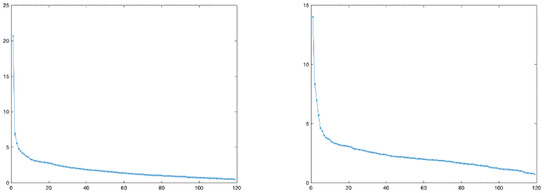
To see why the TTOI iterations yield better estimation than the classic TT-SVD method, recall that TT-SVD first performs singular value thresholding on , i.e., the unfolding of , without any additional updates (see detailed procedure of TT-SVD and formal definition of in Section II-A), which can be inaccurate since , a matrix, has a great number of columns. In contrast, TTOI iteration utilizes the intermediate outcome of the previous iteration to substantially reduce the dimension of while performing singular value thresholding. In Figure 1, we provide a simple simulation example to show that even one TTOI iteration can significantly improve the estimation of the left singular subspace of G1 (left panel) and the overall tensor (right panel). Therefore, a one-step TTOI, i.e., the initialization with one TTOI iteration, can be used in practice when the computational cost is a concern.
Fig. 1.
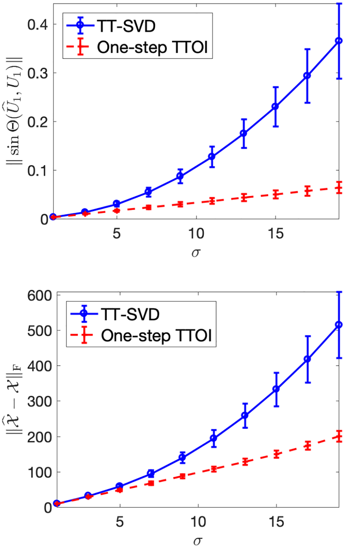
Average estimation error (dots) and standard deviation (bars) of and by TT-SVD and one-step TTOI. Both algorithms are performed based on the observation generated from (2), where , is a randomly generated order-5 tensor based on (1) with p = 20, r = 1, G1, , .
We develop theoretical guarantees for TTOI. In particular, we introduce a series of representation lemmas for tensor matricizations with TT format. Based on them, we develop a deterministic upper bound of estimation error for both forward and backward updates in TTOI iterations. Under the benchmark setting of spiked tensor model, we develop matching upper/lower bounds and prove that the proposed TTOI algorithm achieves the minimax optimal rate of estimation error. To the best of our knowledge, this is the first statistical optimality results for high-order tensors with TT format. We also prove for any high-order tensor, TTOI iteration has monotone decreasing approximation error with respect to the iteration index.
Moreover, to break the curse of dimensionality in high-order Markov processes, we study the state aggregatable high-order Markov processes and establish a key connection to TT decomposable tensors. We propose a TTOI estimator for the transition probability tensor in high-order state-aggregatable Markov processes and establish the theoretical guarantee. We conduct simulation experiments to demonstrate the performance of TTOI and validate our theoretical findings. We also apply our method to analyze a New York taxi dataset. By modeling taxi trips as trajectories realized from a citywide Markov chain, we found that the Manhattan traffic zone exhibits high-order Markovian dependence and the proposed TTOI reveals latent traffic patterns and meaningful partition of Manhattan traffic zones. Finally, we discuss several applications that our proposed algorithm is applicable to, including transition probability tensor estimation in high-order Markov decision processes and joint probability tensor estimation in Markov random fields.
C. Related Literature
In addition to the aforementioned literature on TT decomposition, our work is also related to a substantial body of work on matrix/tensor decomposition and SVD, spiked tensor model, etc. These literature are from a range of communities including applied mathematics, information theory, machine learning, scientific computing, signal processing, and statistics. Here we try to review existing literature in these communities without claiming this literature survey is exhaustive.
First, the matrix singular value thresholding was commonly used and extensively studied in various problems in data science, including matrix denoising [37], [38], [39], matrix completion [40], [41], [42], [43], principal component analysis (PCA) [44], Markov chain state aggregation [45]. Such the task was also widely considered for tensors of order-3 or higher. In particular, to perform SVD and decomposition for tensors with Tucker low-rank structures, [46], [47] introduced the higher-order SVD (HOSVD) and higher-order orthogonal iteration (HOOI). [48] established the statistical and computational limits of tensor SVD, compared the theoretical properties of HOSVD and HOOI, and proved that HOOI achieves both statistical and computational optimality. [49] introduced the sequentially truncated higher-order singular value decomposition (ST-HOSVD). [50] introduced a thresholding & projection based algorithm for sparse tensor SVD. A non-exhaustive list of methods for SVD and decomposition for tensors with CP low-rank structures include alternating least squares [51], [52], eigendecomposition-based approach [53], enhanced line search [54], power iteration with SVD-based initialization [6], simultaneous diagonalization and higher-order SVD [55].
In addition, the spiked tensor model and tensor principal component analysis (tensor PCA) are widely discussed in the literature. [56], [57], [58], [59], [60], [61] considered the statistical and computational limits of rank-1 spiked tensor model. [62] studied the statistical and computational phase transitions and theoretical properties of the approximate message passing algorithm (AMP) under a Bayesian spiked tensor model. [63], [64] developed the regularization-based methods for tensor PCA. [65], [66], [67], [68] studied the robust tensor PCA to handle the possible outliers from the tensor observation.
Different from Tucker and CP decompositions, which have been a pinpoint in the enormous existing literature on tensors, we focus on the TT-structure associated with high-order tensors for the following reasons: (1) Tucker and CP decompositions do not involve the sequential structure of different modes, i.e., the Tucker and CP decompositions still hold if the d modes are arbitrarily permuted. While in applications such as high-order Markov process, high-order Markov decision process, and fully connected layers of deep neural networks, the order of different modes can be crucial; (2) the number of entries involved in the low-Tucker-rank parameterization grows exponentially with respect to the order d (rd); (3) methods that explore CP low-rank structure can be numerically unstable for high-order tensors in computation as pointed out by [27]. In comparison, the TT-structure incorporates the order of different modes sequentially and involves much fewer parameters for high-order tensors, which renders it more suitable in many scenarios.
In Section V, we will further discuss the application of TTOI on high-order Markov processes and state aggregation. This problem is related to a body of literature on dimension reduction and state aggregation for Markov processes that we will discuss in Section V.
D. Organization
The rest of the article is organized as follows. In Section II, after a brief introduction of the notation and preliminaries, we introduce the procedure of the tensor-train orthogonal iteration. The theoretical results, including three representation lemmas, a general estimation error bound, and the minimax optimal upper and lower bounds under the spiked tensor model, are provided in Sections III and IV. The application to high-order Markov chains is discussed in Section V. The simulation and real data analysis are provided in Sections VI-A and VI-B, respectively. Discussions and further applications to Markov random fields and high-order Markov decision processes are briefly discussed in Section VII. All technical proofs are provided in Section A.
II. Procedure of Tensor-Train Orthogonal Iteration
A. Notation and Preliminaries
We first introduce the notation and preliminaries to be used throughout the paper. We use the lowercase letters, e.g., x, y, z, to denote scalars or vectors. We use C, c, C0, c0, … to denote generic constants, whose actual values may change from line to line. A random variable z is σ-sub-Gaussian if for any . We say a ≲ b or a = O(b) if a ≲ Cb for some uniform constant C > 0. We write if a = O(b logC′(b)) for constant C′ > 0. The capital letters, e.g., X, Y, Z, are used to denote matrices. Specifically, is the set of all p-by-r matrices with orthogonal columns. For , let be the orthonormal complement of U, and let PU = UU⊤ denote the projection matrix onto the column space of U. For any matrix , let be the singular value decomposition, where are the singular values of A in non-increasing order. Define , , and be the smallest non-trivial singular value, leading r left singular vectors, and leading r right singular vectors of A, respectively. We also write and as the collection of all left and right singular vectors of A, respectively. Define the Frobenius and spectral norms of A as and . For any two matrices and , let
be their Kronecker product. To quantify the distance among subspaces, we define the principle angles between U, as an r-by-r diagonal matrix: , where s1 ≥ ⋯ ≥ sr ≥ 0 are the singular values of . Define the sinΘ norm as
The boldface calligraphic letters, e.g., , , , are used to denote tensors. For an order-d tensor1 and 1 ≤ k ≤ d − 1, we define as the sequential unfolding of with rows enumerating all indices in Modes 1, …, k and columns enumerating all indices in Modes (k + 1), ⋯, d, respectively. That is, for any 1 ≤ k ≤ d and 1 ≤ ik ≤ pk,
where ξ1(i1, …, id; k) = (ik − 1)p1 ⋯ pk−1 + (ik−1 − 1)p1 ⋯ pk−2 + ⋯ + i1 and ξ2(i1, …, id; k) = (id − 1)pk+1 ⋯ pd−1 + (id−1 − 1)pk+1 ⋯ pd−2 + ⋯ + ik+1. Following the convention of reshape function in MATLAB, we define the reshape of any matrix X of dimension p1 ⋯ pk × pk+1 ⋯ pd as an inverse operation of tensor matricization: if . For any two matrices and , we denote and if and only if
We also define the tensor Frobenius norm of as . For any matrix and any tensor , let vec(A) and be the vectorization of A and , respectively. Formally, for any 1 ≤ k ≤ d and 1 ≤ ik ≤ pk,
B. Procedure of Tensor-Train Orthogonal Iteration
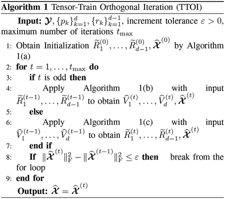
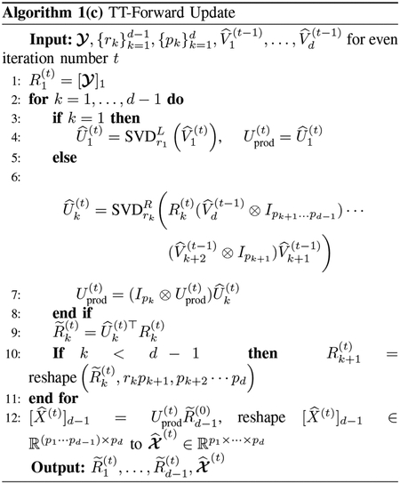
We are now in position to introduce the procedure of Tensor-Train Orthogonal Iteration (TTOI). The pseudocode of the overall procedure is given in Algorithm 1. TTOI includes three main parts: we first run initialization, then perform backward update and forward update alternatively and iteratively.
-
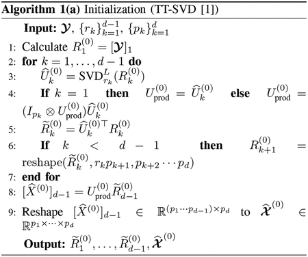
Part 1: Initialization. First, we obtain an initial estimate of TT-cores . This step is the tensor-train-singular value decomposition (TT-SVD) originally introduced by [1].
- Let be the unfolding of along Mode 1. We compute the top-r1 SVD of . Let be the first r1 left singular vectors of and calculate . Then, is an initial estimate of the subspace that G1 lies in and can be seen as the projection residual.
- Next, we realign the entries of to , where the rows and columns of correspond to indices of Modes-1, 2 and Modes-3, …, d, respectively. Then, we evaluate the top-r2 SVD of . Let be the first r2 left singular vectors of and evaluate . Again, is an estimate of the singular subspace that lies on and is the projection residual for the next calculation.
- We apply Step (ii) on to obtain and ; …; apply Step (ii) on to obtain and . Then we reshape matrix to tensor for k = 2, …, d − 1. Now, yield the initial estimates of TT-cores of and we expect that
The initialization step is summarized to Algorithm 1(a) and illustrated in Figure 2. In summary, we perform SVD on some “residual” sequentially for k = 1, …, d − 1. As will be shown in Lemma III.3, satisfies
where is the kth sequential unfolding of (see definition in Section II-A). This quantity plays a key role in the backward update next.The initialization step mainly focuses on the left singular spaces of while ignoring the information included in the right singular spaces. Due to this fact, we develop the following new backward update that utilizes both the left and right singular space estimates from the previous step to refine our estimates. Similarly, we can also perform a forward update to further improve the outcome of backward update, and then iteratively alternate between backward and forward updates. The detailed descriptions of these two updates are presented as follows, and a further explanation is given in Remark II.1.
-
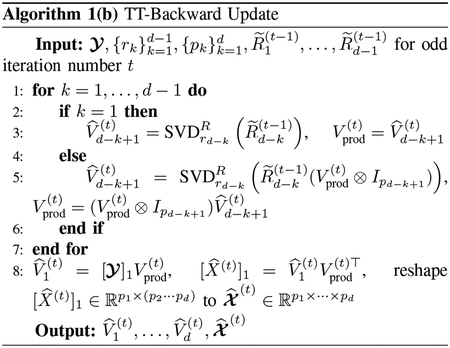
Part 2: Backward update. For iterations t = 1, 3, 5, …, we perform backward update, i.e., to sequentially obtain based on the intermediate results from the (t − 1)st iteration (0th iteration is the initialization). The pseudocode of backward update is provided in Algorithm 1(b). The calculation in Algorithm 1(b) is equivalent to
 for k = d − 1, …, 2, and
Here,
are the projection residual term in the intermediate outcome of the (t − 1)st iteration. Then, we reshape to . The backward up-dated estimate isRemark II.1 (Interpretation of backward update). The backward updates utilize and extract the right singular vectors of the intermediate products of the (t − 1)st iteration,
as opposed to the entire data . Such a dimension reduction scheme is the key to the backward update: it can simultaneously reduce the dimension of the matrix of interest, , and the noise therein, while preserving the signal strength. Different from the initialization in Step 1, the backward update utilizes the information from both the forward and backward singular subspaces of the tensor-train structure of . See Section III for more illustration. -
Part 3: Forward Update. For iteration t = 2, 4, 6, …, we perform forward update, i.e., to sequentially obtain based on the intermediate results from the (t − 1)st iteration. Essentially, the forward update can be seen as a reversion of the backward update by flipping all modes of tensor . The pseudocode of this procedure is collected in Algorithm 1(c). Recall is the intermediate product from the (t − 1)st update. We sequentially compute
for k = 2, …, d − 1, andReshape to for k = 2, …, d − 1. Then, computeWe will explain the algebraic schemes in the TTOI procedure through several representation lemmas in Section III-A. We will also show in Theorem III.2 that the objective function is monotone decreasing with respect to the iteration index t. In the large-scale scenarios that performing iterations is beyond the capacity of computing, we can reduce the number of iterations, and even to tmax = 1, i.e., the one-step iteration, which have often yielded sufficiently accurate estimation as we will illustrate in both theory and simulation studies. Such the phenomenon has been recently discovered for HOOI in the Tucker low-rank tensor decomposition [69].
Remark II.2 (Computational and storage costs of TTOI). We consider the computational and storage costs of TTOI on the p-dimensional, rank-r, order-d, and dense tensor. Since computing the first r singular vectors of an m × n matrix via block power method requires operations, initialization costs operations, each iteration of TTOI, including forward and backward updates, costs O(pdr). Therefore, the total number of operations of TTOI with T iterations is , which is not significantly more than the number of elements of the target tensor. Moreover, TTOI requires O(pd) storage cost, which is not significantly more than the storage cost of the original tensor.
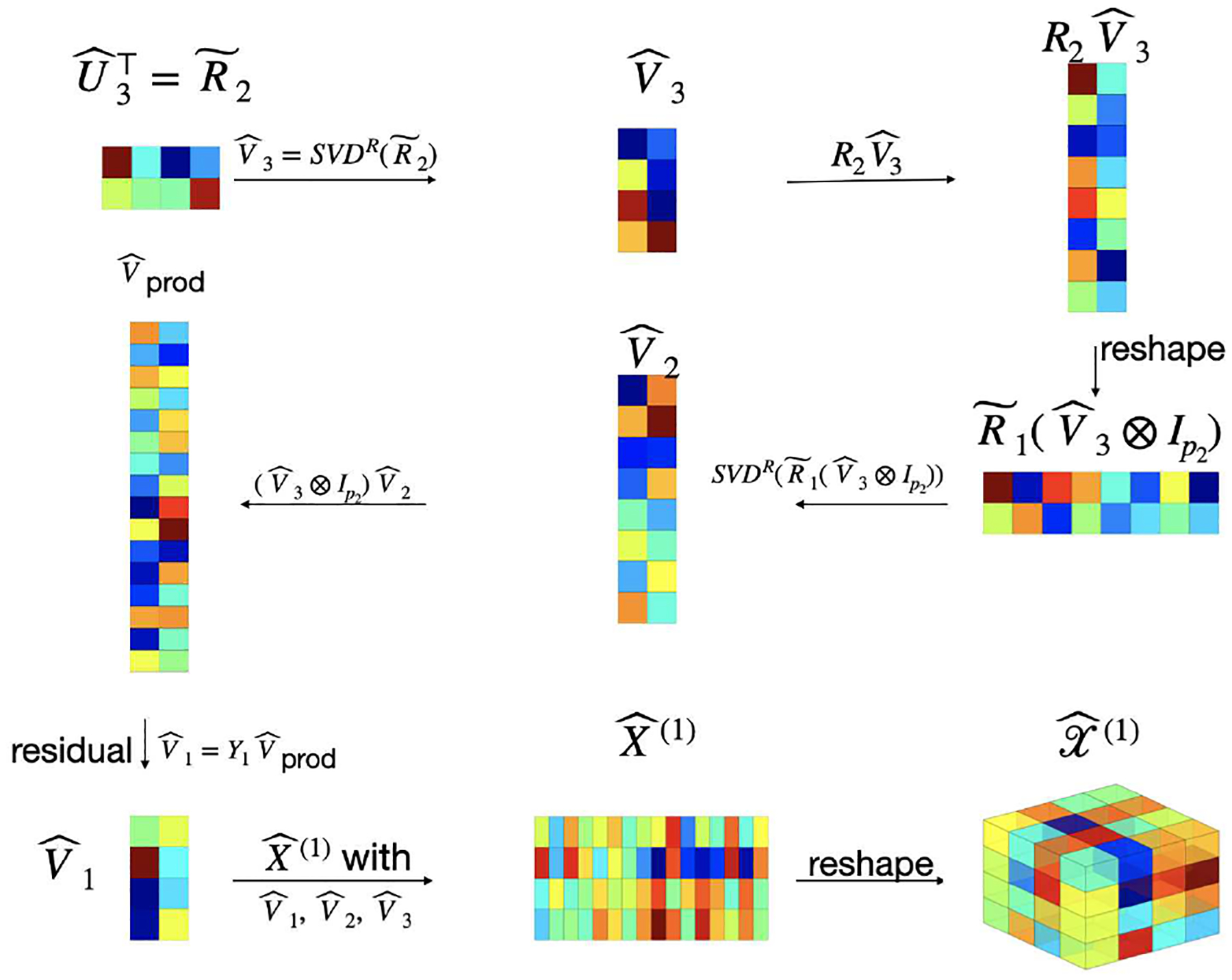
Fig. 2.
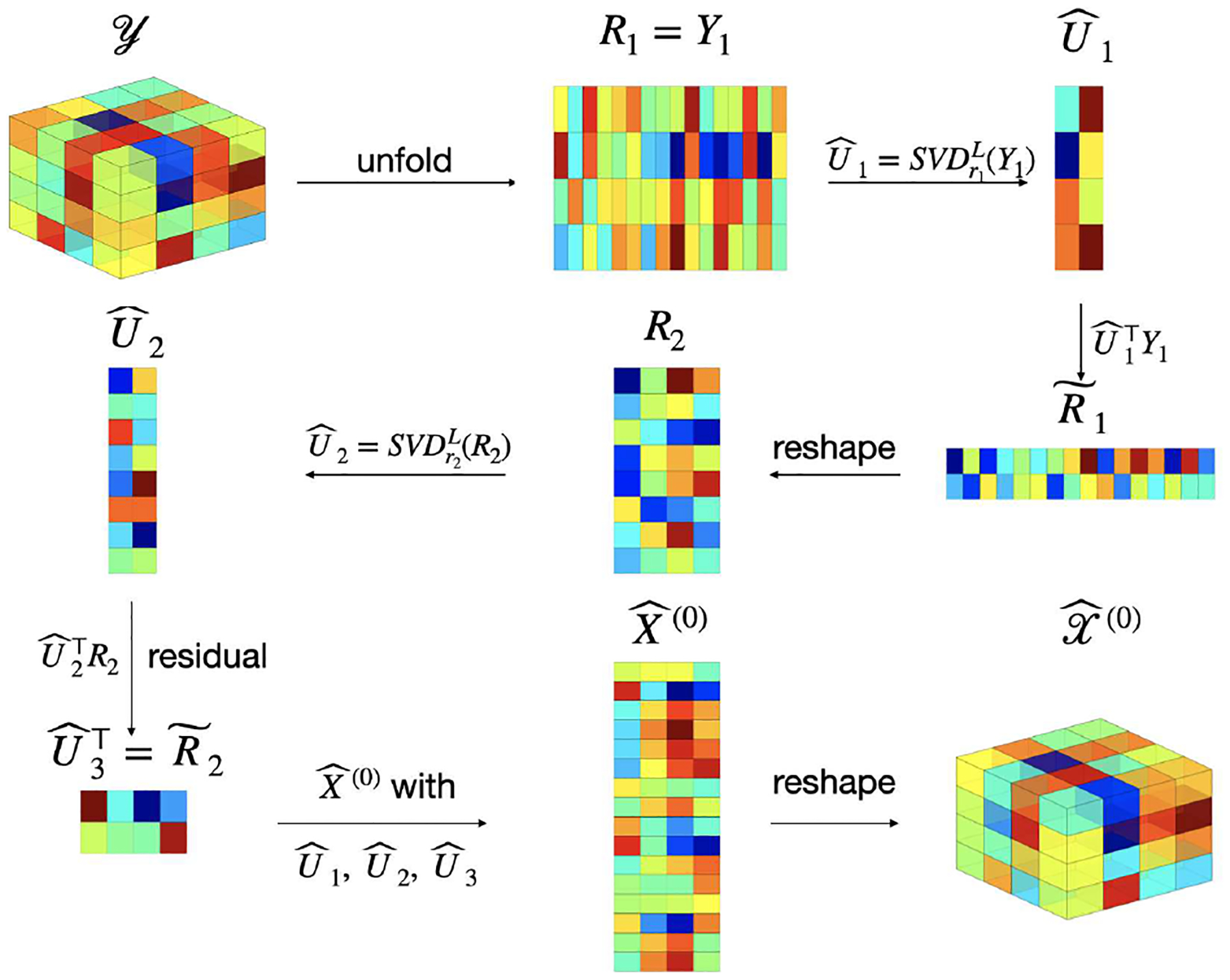
A Pictorial Illustration of Initialization (Algorithm 1(a), d = 3)
III. Theoretical Analysis
This section is devoted to the theoretical analysis of the proposed procedure. For convenience, we introduce the following two abbreviations for matrix sequential products: for , 1 ≤ i ≤ d − 1 and , 2 ≤ j ≤ d, we denote
Equivalently, and can be defined sequentially as
A. Representation Lemmas for high-order tensors
Since the computation of high-order tensors with tensor-train structures involves extensive tensor algebra, we introduce the following three lemmas on the matrix representation of high-order tensors. These lemmas play a fundamental role in the later theoretical analysis.
Lemma III.1 (Representation for sequential matricization of TT-decomposable tensor). Suppose . Then the sequential matricization of can be written as
| (4) |
Lemma III.2 (Representation of tensor reshaping). For any tensor and 1 ≤ i < j ≤ d − 1, we have
Here, we define as the kth canonical basis of and
| (5) |
Lemmas III.1 and III.2 can be proved by checking each entry of the corresponding matricizations. In addition, the following lemma provides a representation of sequential reshaping tensor, in particular for and , the key intermediate outcomes in TTOI procedure.
Lemma III.3 (Representation of sequential reshaping tensor). Suppose , for 1 ≤ i ≤ d − 1, for 2 ≤ i ≤ d, where r0 = rd = 1. Consider the following sequential multiplication:
Forward sequential multiplication: Let . For k = 1, …, d − 1, calculate
Then for any 1 ≤ k ≤ d − 1,
| (6) |
Here, if k = 1.
Backward sequential multiplication: Let . For k = d − 1, …, 1, calculate
Then for any 1 ≤ k ≤ d − 1,
Here, if k = d − 1.
In particular, , in Algorithm 1(a) and , in Algorithm 1(c) satisfy
| (7) |
B. Deterministic Upper Bounds for Estimation Error of TTOI
Now we are in position to analyze the performance of TTOI. The following Theorem III.1 introduces an upper bound on estimation error of (backward update) and (forward update).
Theorem III.1. Suppose we observe , where admits a TT decomposition as (1).
(A deterministic estimation error bound for backward updates) Let be the left singular space of . For 2 ≤ k ≤ d − 1, define as the left singular subspace of . If for some constant c0 ∈ (0, 1),
| (8) |
then there exists a constant Cd > 0 that only depends on d such that the outcome of Algorithm 1(b) satisfies
| (9) |
where
Here, if k = d − 1.
(A deterministic estimation error bound for forward updates) For 2 ≥ k ≤ d − 1, let be the right singular space of and let be the right singular space of . If for some constant c0 ∈ (0, 1),
then there exists a constant Cd > 0 that only depends on d such that the outcome of Algorithm 1(c) satisfies
| (10) |
where
Here, if k = 1.
The proof of Theorem III.1 is provided in Section A-A. Theorem III.1 shows the estimation error can be bounded by the projected noise , i.e., and B(t+1), if the estimates in initialization (t = 0) or the previous iteration (t ≥ 1), or , are within constant distance to the true underlying subspaces. The developed upper bound can be significantly smaller than , the classic upper bound induced from the approximation error (e.g., Theorem 2.2 in [1]), especially in the high-dimensional setting (p ≫ r).
Remark III.1 (Interpretation of error bounds in Theorem III.1). Here, we provide some explanation for and B(2t+1) in the error bound (9). By algebraic calculation, the TT-core estimation via backward update can be written as
for any 1 ≤ k ≤ d − 1 and
From the definition of , we have see quantifies the error of the singular subspace estimate and B(2t+1) quantifies the error of the projected residual . By symmetry, similar interpretation also applies to and B(2t+2) for the error bound of forward update (10).
Remark III.2 (Proof Sketch of Theorem III.1). While the complete proof of Theorem III.1 is provided in Section A-A, we provide a brief proof sketch here.
Without loss of generality, we focus on (9) for t = 0 while other cases follows similarly. For convenience, we simply let , denote , , respectively. First, by Lemma III.1, we can transform , the outcome of backward update, to
Then we can further bound the estimation error of as
Next, based on Lemma III.2 and (8), we can prove
Finally, we apply the perturbation projection error bound (Lemma A.3) to prove that
Theorem (IV.1) is proved by combing all inequalities above.
Next, we establish a decomposition formula for the approximation error, i.e., the objective function in (3) , and show that the approximation error is monotone decreasing through TTOI iterations.
Theorem III.2 (Approximation error decays through iterations). We implement TTOI on . Let be the outcome after the tth iteration. For any k ≥ 1, we have
| (11) |
| (12) |
IV. TTOI for Tensor-Train Spiked Tensor Model
In this section, we further focus on a probabilistic setting, spiked tensor model, where the noise tensor has independent, mean zero, and σ-sub-Gaussian entries (see definition in Section II-A). The spiked tensor model has been widely studied as a benchmark setting for tensor PCA/SVD and dimension reduction in recent literature in machine learning, information theory, statistics, and data science [62], [61], [60], [70], [48]. The central goal therein is to discover the underlying low-rank tensor . Most of the existing works focused on tensors with Tucker or CP decomposition.
Under the spiked tensor model, we can verify that the initialization step of TTOI gives sufficiently good initial estimations with high probability that matches the required condition in Theorem III.1.
Theorem IV.1 (Probabilistic bound for initial estimates and projected noise). Suppose is TT-decomposable as (1) and have independent zero mean and σ-sub-Gaussian random variables. Denote p = min{p1, ⋯, pd}. If there exists a constant Cgap such that for 1 ≤ k ≤ d − 1, then there exist some constants C, c > 0 and Cd > 0 that only depends on d, with probability at least 1 − C exp(−cp),
| (13) |
| (14) |
and for all t ≥ 1,
| (15) |
Here, , , and B(t) are defined in Theorem III.1.
The proof of Theorem IV.1 is provided in Section A–C. Based on Theorems III.1 and IV.1, we can further prove:
Corollary IV.1 (Upper bound for estimation error). Suppose can be decomposed as (1), are independent zero mean and σ-sub-Gaussian random variables, p = min{p1, ⋯, pd}. Suppose there exists a constant Cgap such that for 1 ≤ k ≤ d − 1. Then with probability at least 1 − Ce−cp, for all t ≥ 1,
| (16) |
The proof of Corollary IV.1 is provided in Section A–D.
Remark IV.1 (Interpretation of Corollary IV.1). Note that the TT-cores G1, , Gd respectively have p1r1, piriri−1, pdrd−1 free parameters, the upper bound (16) can be seen as the noise level σ2 times the degrees of freedom of the low TT rank tensors.
Next, we develop a minimax lower bound for the low TT rank structure estimation. Consider the following general class of tensors with dimension p = (p1, …, pd) and TT rank r = (r1, …, rd−1),
| (17) |
and a class of distributions of σ-sub-Gaussian noise tensors
| (18) |
Here, the constraints on the least singular value of and the σ-sub-Gaussian assumption correspond to the conditions required for upper bound in Theorem IV.1.
Theorem IV.2 (Lower bound). Consider the order-d TT spiked tensor model (2) and distribution class in (18). Assume p = min{p1, …, pd} ≥ C0 for some large constant C0, r1 ≤ p1/2, ri ≤ piri−1/2, ri−1 ≤ piri/2 for 2 ≤ i ≤ d − 1, rd−1 ≤ pd, and λi > 0. Also assume r1r2 ≤ p1 if d = 3. Then there exists a constant cd > 0 that only depends on d such that
| (19) |
V. TTOI for Dimension Reduction and State Aggregation in High-order Markov Chain
Since the introduction at the beginning of the 20th century, the Markov process has been ubiquitous in a variety of disciplines. In the literature, the first order Markov process, i.e., the future observation at (t + 1) is conditionally independent of those at times 1, …, (t − 1) given the immediate past observation at time t, has been commonly used and extensively studied. Moreover, the high-order Markov process often appear in many scenarios, where the future observation is affected by a longer history. For example, in the taxi travel trajectory, the future stop of a taxi not only depends on the current location but also the past path that reveals the direction this taxi is heading to [71]. The high-order Markov processes have also been applied to inter-personal relationship [72], financial econometrics [73], traffic flow [74], among many other applications.
We specifically consider an ergodic, time-invariant, and (d − 1)st order Markov process on a finite state space {1, …, p}. That is, the future state Xt+d depends on the current state Xt+d−1 and the previous (d − 2) states (Xt+d−2, …, Xt+1) jointly:
| (20) |
Our goal is to achieve a reliable estimation of the transition tensor and to predict the future state Xt+d based on an observable trajectory. Since the total number of free parameters in a (d − 1)st order Markov transition tensor is O(pd) without further assumptions, it may be prohibitively difficult to infer in both statistics and computation even if p and d are only of moderate scale. Instead, a sufficient dimension reduction for high-order Markov processes is in demand.
To enable the statistical inference and dimension reduction for high-order Markov processes, a powerful tool, mixed transition distribution model (MTD), was introduced [72]. The MTD model assumes that the distribution of future state is a linear combination of the distributions associated with the (d − 1) immediate past states. The readers are also referred to [75] for a survey on mixed transition distribution model. The linear assumption, however, does not take into account the potential interactions of past states that commonly appear in practice. For example in the New York taxi trip data, the interaction among past locations of a taxi indicates its potential future direction.
On the other hand, there is a recent surge of development in dimension reduction and state aggregation for first order Markov chains. For example, [76] considered the Markov chain aggregation and the application to biology; [77] considered the rank-reduced Markov model and mode clustering; [45] considered Markov rank, aggregagability, and lumpability of Markov processes and proposed the dimension reduction and state aggregation methods through spectral decomposition with theoretical guarantees; [78] proposed clustering block model and proposed efficient algorithm to solve it; [79] introduced a convex and non-convex methods to estimate the rank-reduced low-rank Markov transition matrix.
Inspired by these work, we propose and study the state aggregation model for the discrete-time high-order Markov processes as follows.
Definition V.1 ((d − 1)st order state aggregatable Markov1 process). Suppose there exist maps , , such that G2, …, Gd are linear: Gk(X, λ1u + λ2v) = λ1Gk(X, u) + λ2Gk(X, v) for any vectors u, v, scalars . We say a Markov process {X1, X2, …} is (d − 1)st order state aggregatable if for all t ≥ 0, the transition can be sequentially generated as follows,
In a (d − 1)st order state aggregatable Markov process, the future state Xt+d relies on a sequential aggregation of the previous d − 1 states Xt+1, …, Xt+d−1 as follows: we first project Xt+1 to a r1-dimensional vector via G1, then project jointly with Xt+2 to a r2-dimensional vector via G2. We repeat such the projection sequentially for Xt+3, …, Xt+d and yield the transition probability . Also, see Figure 4 for a pictorial illustration.
Fig. 4.
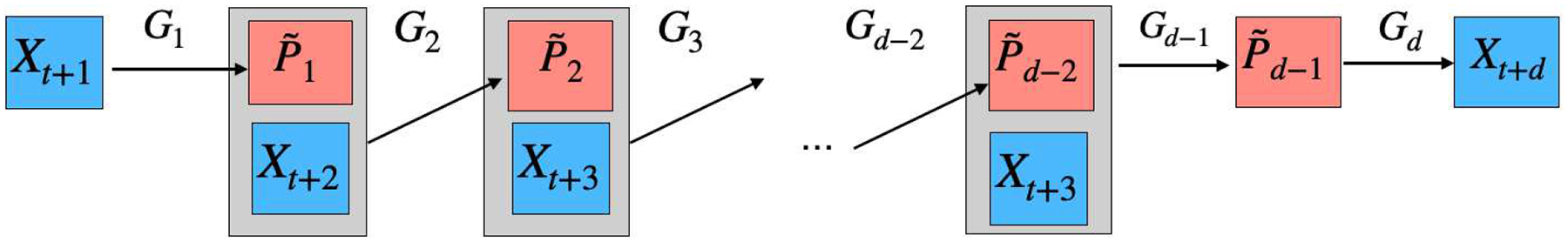
A pictorial illustration of a (d − 1)st order state aggregatable Markov chain
Based on the definition of the state aggregatable Markov chain, we can prove the corresponding probability transition tensor will have low TT rank.
Proposition V.1. The transition tensor of the rank reduced high-order Markov model in Definition V.1 has TT-rank no more than (r1, …, rd−1). In other words, satisfies .
The proof of Proposition V.1 is provided in Section A–F.
Next, we focus on a synchronous or generative setting, which can be seen as a high-order generalization of the classic observation model for the analysis of Markov (decision/reward) processes (see [80] for an introduction), for the high-order Markov process. To be specific, for each sample index k = 1, …, n and previous states (i1, …, id−1) ∈ [p]d−1, suppose we observe the next state X(i1, …, id−1; k) drawn from the Markov transition tensor . It is natural to estimate via the empirical transition tensor: for i1, …, id ∈ {1, …, p}d,
Then, is an unbiased estimator of . However, if the entries of are approximately balanced, the mean squared error of satisfies
| (21) |
To obtain a more accurate estimator, we propose to first perform TTOI on to obtain , then project each row of , or equivalently, each mode-d fiber of , onto the simplex via probability simplex projection (see an implementation in [81]) and obtain .
We establish an upper bound on estimation error for the TTOI estimator .
Proposition V.2. Consider the synchronous or generative model for a (d − 1)st order state aggregatable Markov process described above. Suppose the initialization condition (8) in Theorem III.1 holds. Then with probability at least 1 − Ce−cp, the output of one-step TTOI followed by the probability simplex projection satisfies
The proof of Proposition V.2 is provided in Section A–G. Compared to the estimation error rate of in (21), Proposition V.2 shows TTOI achieves significantly reduced estimation error by exploiting the low TT rank structure of the high-order Markov process.
Remark V.1. If the observations form one transition trajectory {X0, …, XN}, we can work on the following empirical transition tensor:
| (22) |
Then can be a nearly unbiased and strongly consistent estimator for . When the Markov process is (d − 1)st order state aggregatable, we can apply TTOI to obtain a better estimate. As will be explored by numerical studies in Section VI-A, the TTOI estimator achieves favorable performance on the estimation of .
VI. Numerical Studies
In this section, we investigate the numerical performance of TTOI.
A. Simulation
In each simulation setting, we present the numerical results in both average estimation error (denoted by dots) and standard deviation (denoted by bars) based on 100 repetitions. We assume the true TT-ranks are known in the first three settings. Afterwards, we introduce a BIC-type data-driven scheme for TT-rank selection and present its numerical performance. All experiments are conducted by a quad-core 2.3 GHz Intel Core i5 processor.
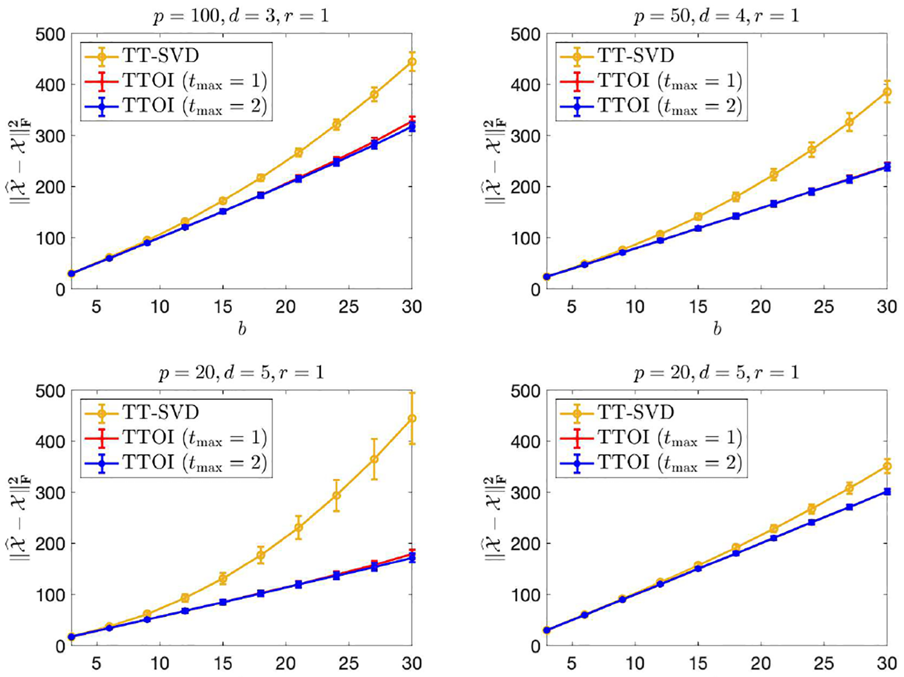
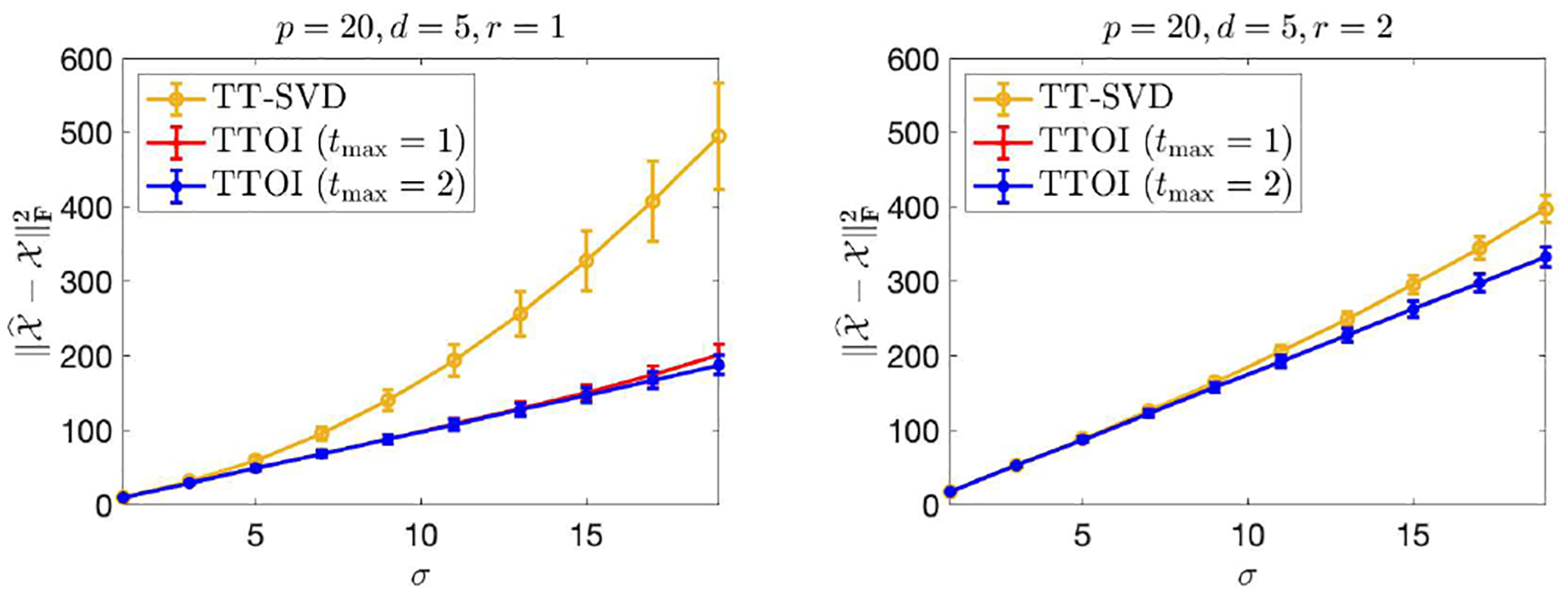
We first consider the tensor-train spiked tensor model (2) discussed in Section IV. Specifically, we randomly generate with i.i.d. standard normal entries, and generate with i.i.d. or Unif(−b, b) entries. Let p1 = ⋯ = pd = p, r1 = ⋯ = rd−1 = r, and consider four settings: (1) p = 100, d = 3, r = 1; (2) p = 50, d = 4, r = 1; (3) p = 20, d = 5, r = 1; (4) p = 20, d = 5, r = 2. For varying values of σ ∈ [1, 19] and b ∈ [3, 30], we evaluate the estimation error of the TT-SVD and TTOI estimators with 1 or 2 iterations, i.e., tmax = 0, 1, 2. From the results summarized in Figure 5 (normal noise) and Figure 6 (uniform noise), we can see TTOI, even with one iteration, performs significantly better than TT-SVD, and the advantage becomes more significant as the noise level σ, b grows. This suggests that the proposed TTOI is effective for high-order tensor SVD compared to the classic TT-SVD, especially when the observations are corrupted by substantial noise. Table I summarizes the runtime of TT-SVD and TTOI, which suggests that the additional computational cost incurred by the backward and forward updates in TTOI is negligible compared to the runtime of the original TT-SVD.
Fig. 5.
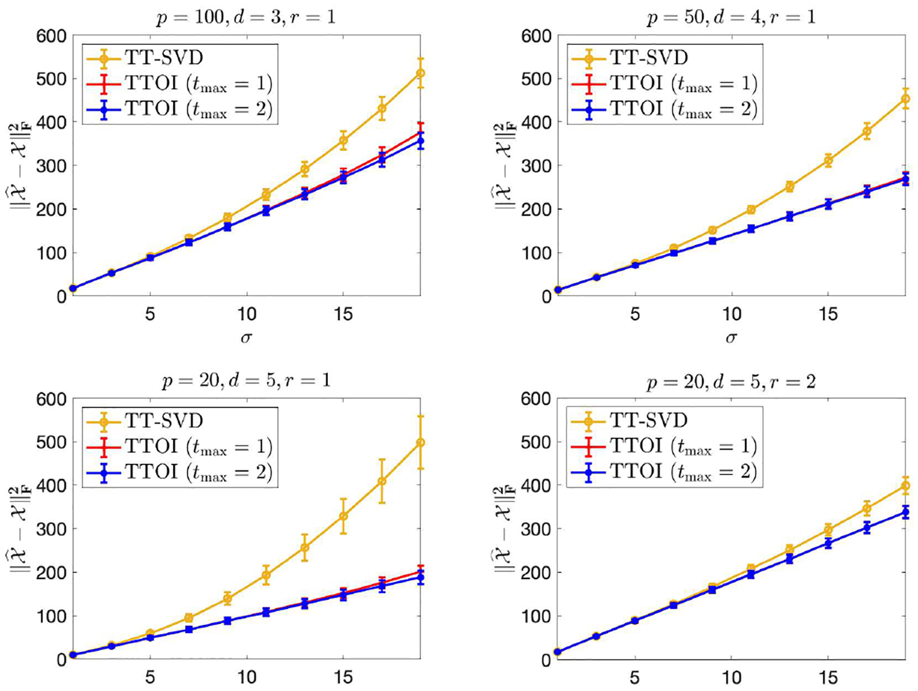
Estimation error of TT-SVD and TTOI for high-order spiked tensor model. Here, .
Fig. 6.
Estimation error of TT-SVD and TTOI for high-order spiked tensor i.i.d. model. Here, .
TABLE I.
Runtime (in seconds) of TT-SVD, TTOI with 1 iteration, and TTOI with 2 iterations under the high-order spiked tensor model with . The mean runtime of 50 independent replicates are presented and the standard deviations are listed in parentheses.
| (p, d, r) | TT-SVD | TTOI (tmax = 1) | TTOI (tmax = 2) |
|---|---|---|---|
| (100, 3, 1) | 0.332 (0.071) | 0.334 (0.071) | 0.340 (0.074) |
| (50, 4, 1) | 1.165 (0.173) | 1.169 (0.172) | 1.201 (0.171) |
| (20, 5, 1) | 0.725 (0.093) | 0.730 (0.092) | 0.751 (0.095) |
| (20, 5, 2) | 0.672 (0.100) | 0.676 (0.101) | 0.708 (0.103) |
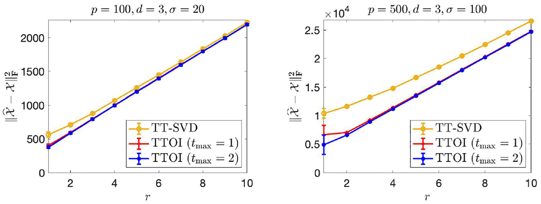
To understand the influence of TT-rank to the performance of the TT-SVD and TTOI estimators, we conduct numerical experiments under the spiked tensor model (2) with r1 = ⋯ = rd−1 = r for various values of r. In particular, are still generated with i.i.d. standard normal entries, and has i.i.d. entries. Letting p1 = ⋯ = pd = p, we consider two settings: (1) p = 100, d = 3, σ = 20; (2) p = 500, d = 3, σ = 100. For r = 1, …, 10, we evaluate the average estimation error of TT-SVD, TTOI with 1 iteration, and TTOI with 2 iterations (i.e., tmax = 0, 1, 2), and present the results in Figure 7. Figure 7 suggests that the estimation errors increase as the rank increases, while TTOI with 1 or 2 iterations both performs better than TT-SVD. The improvement of TTOI over TT-SVD is more significant under larger p or smaller r. An intuitive explanation for this phenomenon is as follows: the key idea of TTOI is to utilize the previous updates to reduce the dimension of the sequential unfolding before performing singular value thresholding; such the dimension reduction is more significant for large p or small r.
Fig. 7.
Estimation error of TT-SVD and TTOI for high-order spiked tensor model with varying TT-ranks
Next, we demonstrate the performance of TTOI on transition tensor estimation for the high-order state-aggregatable Markov chains studied in Section V. We consider the (d − 1)st order Markov chain on p states. To generate the transition tensor , we first draw , with i.i.d. standard normal entries, then normalize the rows of in absolute values as
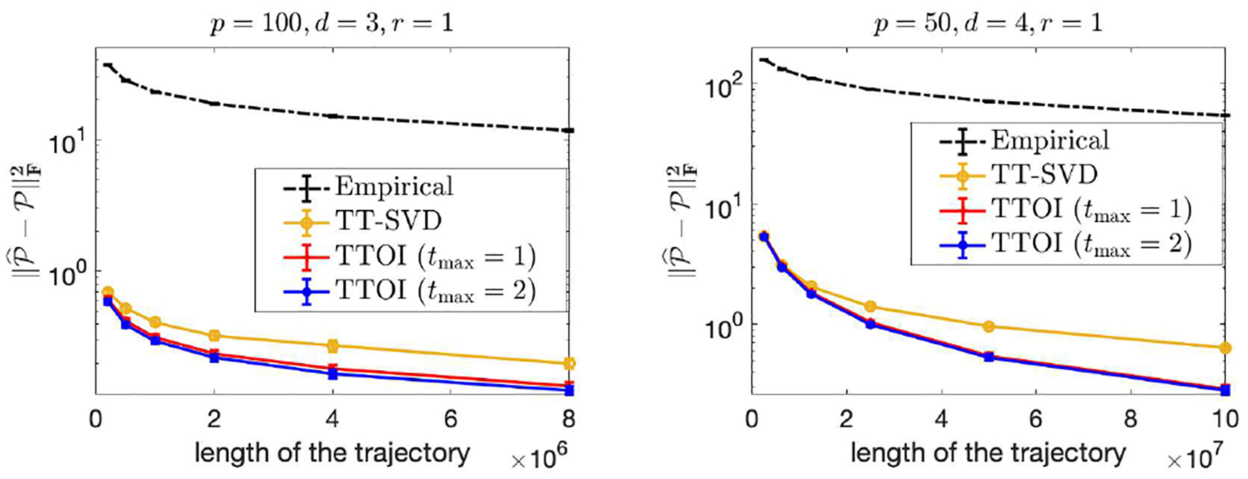
By this means, satisfies , for any (i1, …, id−1), so forms a Markov transition tensor. To generate the trajectory {X1, …, XN}, we generate the initial d − 1 states X1, …, Xd−1 i.i.d. uniformly from [p], then generate Xd, …, XN sequentially according to (20). To estimate , we construct the empirical probability tensor by (22), then apply TT-SVD and TTOI with input as detailed in Section V to obtain . We consider two numerical settings: (1) p = 100, d = 3, r = 1; (2) p = 50, d = 4, r = 1. We evaluate the estimation error for each setting and summarize the results to Figure 8. Again, TTOI exhibits clear advantage over the existing methods in all simulation settings.
Fig. 8.
Estimation error of the transition tensor versus length of the observable trajectory in high order state-aggregatable Markov chain estimation.
Selection of TT-ranks. The proposed TTOI algorithm requires specifying TT-ranks r1, …, rd−1 as inputs and the appropriate choices of r1, …, rd−1 are crucial in practice. We propose a data-driven scheme to select the TT-ranks: we choose r1, …, rd−1 ≥ 1 such that the following Bayesian information criterion (BIC) under the spiked tensor model is minimized:
| (23) |
Here, is the output of TTOI (Algorithm 1) with the input TT-ranksb r1, …, rd−1. This BIC-type criterion was also adopted in prior works on tensor clustering [82].
Then we conduct numerical experiments under the same setting as the bottom two plots in Figure 5 on the spiked tensor model with Gaussian noise. Figure 9 summarizes the estimation errors of TT-SVD and TTOI with 1 and 2 iterations, respectively, with the ranks selected based on the proposed BIC criterion (23). Comparing Figure 9 to the bottom two plots in Figure 5, we can see the proposed criterion can select the true ranks accurately and the performance of both TT-SVD and TTOI with tuned ranks is very similar to the one by inputting the true ranks.
Fig. 9.
Average estimation error of TT-SVD and TTOI for high-order spiked tensor model with BIC-tuned ranks.
B. Real Data Experiments
We apply the proposed method to investigate the Manhattan taxi data. This dataset contains the New York City taxi trip records from 14,144 drivers in 2013. We treat each travel record as a transition among different locations at New York City, then the overall dataset can be organized as a collection of fragmented sample trajectories of a Markov chain on New York City traffic. Some recent analysis on such data can be seen at, e.g., [71], [83], [45].
Due to the high-dimensional spatiotemporal nature of the dataset, a sufficient dimension reduction or state aggregation is often a crucial first step to study a metropolitan-wide traffic pattern. To this end, we apply the high-order Markov model as described in Section V. Specifically, we discretize the Manhattan region into a grid of p = 119 states that forms a state space. Then, we collect all travel records in Manhattan of each driver from the dataset, sort them by time, and form into Markovian transition trajectories. In particular, each travel record is treated as a transition from the pickup to the drop-off location. If the drop-off location i of the previous trip is different from the pickup location j of the next trip by the same driver, we also form a transition from states i to j. Based on the trajectories, we can construct a high-order Markov chain with an order d empirical transition probability tensor as described in Section V. Assuming the true probability tensor is state aggregatable (Definitionb V.1), we apply one-step TTOI proposed in Section V and obtain . It is noteworthy if d = 2, the described procedure of is equivalent to the classic matrix spectral decomposition in the literature. Figure 10 plots the singular values of the sequential unfolding matrices of for d = 3, which clearly demonstrates the low-TT-rankness of the probability transition tensor . In the following experiments, we focus on the order-2 Markov model and analyze all consecutive two transitions: i → j → k, corresponding to the d = 3 case.
Fig. 10.
Singular values of sequential unfolding matrices (left panel) and (right panel)
Inspired by the classic methods of matrix spectral decomposition, we aggregate all location states in Manhattan into a few clusters via both and . Specifically, we calculate , i.e., the last TT-core of , and , i.e., the matricization of whose columns correspond to the last mode. Then we perform k-means on all columns of and , record the cluster index, associate the index to each location state, and plot the results in Figure 11 (Panels (a)(b) are for TTOI and Panels (c)(d) are for empirical estimate). From Figure 11 (a)(b), we can clearly identify four regions: (i) lower Manhattan (orange), (ii) midtown (dark blue), (iii) upper west side (green), and (iv) upper east side (brown or black). In contrast, direct clustering on yields less interpretable results as the majority points go to one cluster. It is also worth noting even the location information is not provided to this experiment, the resulting clusters in Figures 11 (a)(b) show good spatial proximity between locations. This illustrates the effectiveness of TTOI in dimension reduction and state-aggregation for high-order Markov processes.
Fig. 11.
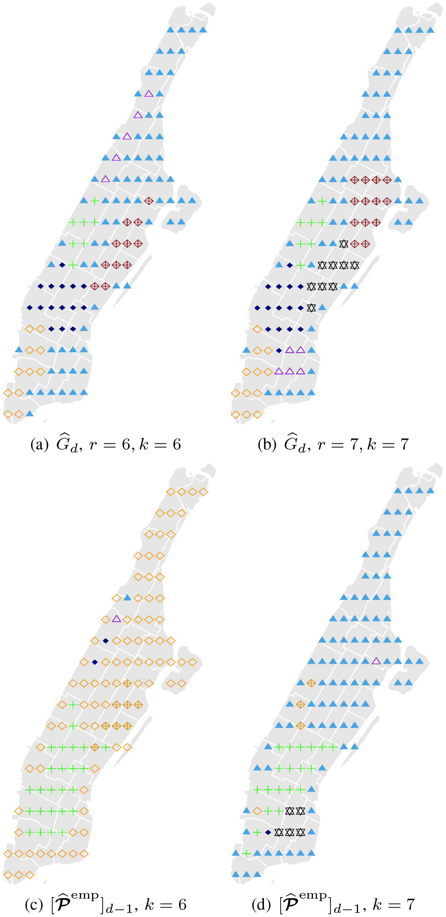
State aggregation based on TTOI and empirical estimate
Next, we illustrate the high-order nature of the city-wide taxi trip through the following experiment. For each initial state i ∈ [p], we apply k-means to cluster the column span of , where is the outcome of TTOI. We present the results in Figure 12, where the red triangles denote the given first state i and r = k = 7. If the city-wide taxi trips do not have significant high-order effects, should be reducible to a first order Markov process and should have similar values for different i. However, as we can see from Figure 12 that the clustering results highly depends on the first state i, the high-order effects exist in the city-wide taxi trip Markov process. In addition, the states in different directions of i are often clustered to different regions, which shows that the taxi drivers may tend to move to the same direction in consecutive trips, which yields the high-order effects in the driving trajectories.
Fig. 12.
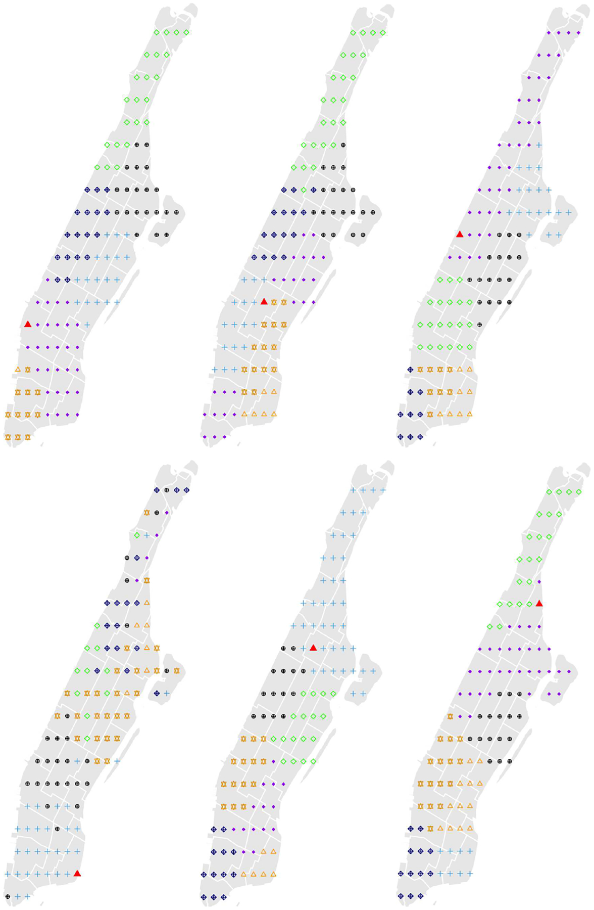
Based on second order Markov model, state aggregation results are different with different initial state (the red triangle denotes the initial state i in each subfigure)
VII. Discussions and Additional Applications
In this paper, we propose a general framework for high-order SVD. We introduce a novel procedure, tensor-train orthogonal iteration (TTOI), that efficiently estimates the low tensor train rank structure from the high-order tensor observation. TTOI has significant advantages over the classic ones in the literature. We establish a general deterministic error bound for TTOI with the support of several new representation lemmas for tensor matricizations. Under the commonly studied spiked tensor model, we establish an upper bound for TTOI and a matching information-theoretic lower bound. We also illustrate the merits of TTOI through simulation studies and a real data example in New York City taxi trips.
In addition to the high-order Markov processes, the proposed TTOI can also be applied to the Markov random field (MRF) estimation. We give a brief description of MRF below. Consider an undirected graph G = (V, E), where V = {1, …, d} is a set of vertices and E ⊆ V × V is a collection of edges. Each vertex i ∈ V is associated with a random variable Xi, taking values in {s1, …, sp}. In an MRF model, the distribution of {X1, …, Xd} can be factorized as
where is a collection of subgraphs of G and XC = (Xv, v ∈ C) denotes the random vector corresponding to vertices in C. The joint probability function can be written as a tensor , where . The MRFs have a wide range of applications, including image analysis [84], [85], genomic study [86], and natural language processing [87]. The readers are referred to, e.g., [88] for an introduction to MRFs.
A central problem of MRF is how to estimate the population density based on a limited number of samples . It is straightforward to estimate via the empirical probability tensor :
We can show that is unbiased for . Recently, [17] pointed out that is often approximately low tensor-train rank in practice. To further exploit such the structure, we can conduct TTOI on . Under regularity conditions, it can be shown that the entries of are bounded and weakly independent, then Corollary IV.1 suggests the following estimation error rate of the TTOI estimator: , which can be significantly smaller than the estimation error of original empirical estimator .
Moreover, the proposed framework can be also applied to high-order Markov decision process (high-order MDP). MDP has been commonly used as a baseline in control theory and reinforcement learning [89], [90], [91], [92]. Despite the wide applications of MDPs, most of the existing work focus on the first-order Markov processes. However, the high-order effects often appear, i.e., the transition probability at the current time depends not only on current, but also the past (d − 1) states and actions. See Figure 13 for an example. Since the number of free parameters in such MDPs can be huge, a sufficient dimension reduction for the state and action space can be a crucial first step. Similarly to the example of high-order Markov process in Section V, the TTOI can be applied to achieve better dimension reduction and state aggregation for the high-order Markov decision processes.
Fig. 13.
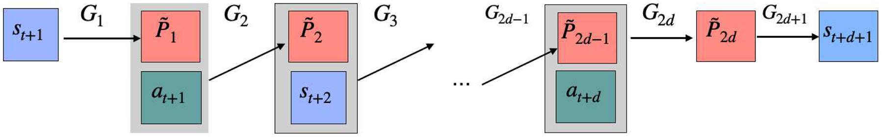
Illustration of a high-order state aggregatable Markov decision process
Fig. 3.
A pictorial illustration of TT-Backward update (Algorithm 1(b), d = 3)
Acknowledgments
The research of Yuchen Zhou and Anru R. Zhang were supported in part by NSF under Grants CAREER-1944904, DMS-1811868, and NIH under Grant R01 GM131399; the research of Yazhen Wang was supported in part by NSF under Grants DMS-1707605 and DMS-1913149. This work was done while Yuchen Zhou, Anru R. Zhang, and Lili Zheng were at the University of Wisconsin-Madison.
Biographies
Yuchen Zhou is a postdoctoral researcher in the Department of Statistics and Data Science, The Wharton School, University of Pennsylvania. He received the B.E. degree from Peking University in 2016 and the Ph.D. degree in statistics from the University of Wisconsin-Madison in 2021. His research interests include high-dimensional statistical inference, tensor data analysis, reinforcement learning and statistical learning theory.
Anru R. Zhang is the Eugene Anson Stead, Jr. M.D. Associate Professor in the Department of Biostatistics & Bioinformatics and Associate Professor in the Departments of Computer Science, Mathematics, and Statistical Science at Duke University. He was an assistant professor of statistics at the University of Wisconsin-Madison in 2015–2021. He obtained his bachelors degree from Peking University in 2010 and his Ph.D. from the University of Pennsylvania in 2015. His work focuses on high-dimensional statistical inference, non-convex optimization, statistical tensor analysis, computational complexity, and applications in genomics, microbiome, electronic health records, and computational imaging. He received the ASA Gottfried E. Noether Junior Award (2021), a Bernoulli Society New Researcher Award (2021), an ICSA Outstanding Young Researcher Award (2021), and an NSF CAREER Award (2020).
Lili Zheng is a postdoctoral researcher in the Department of Electrical and Computer Engineering at Rice University. She received her bachelor’s degree from University of Science and Technology of China (USTC) in 2016 and her Ph.D. degree in statistics from University of Wisconsin - Madison in 2021. Her research interests span dependent data, high-dimensional statistics, network analysis, tensor modeling, stochastic algorithms, and non-convex optimization.
Yazhen Wang is Chair and Professor of Statistics at the University of Wisconsin-Madison. He obtained his Ph.D in statistics from University of California at Berkeley in 1992. He is the fellows of Institute of Mathematical Statistics (IMS) and American Statistical Association (ASA). He served on numerous professional committees of ASA, IMS and ICSA, as NSF program director, editors of Statistics Sinica and Statistics and Its Interface, and associate editors of various journals including Annals of Statistics, Annals of Applied Statistics, Journal of the American Statistical Association, Journal of Business and Economic Statistics, and Statistica Sinica. His research interests are financial econometrics, quantum computation, machine learning, high dimensional statistics, nonparametric curve estimation, wavelets, change points, long-memory processes, and order restricted inference.
Appendix A
Proofs
We collect all technical proofs of this paper in this section.
A. Proof of Theorem III.1
For convenience, let , , Ri and denote , , and , respectively. By Lemma III.1 and
we have
| (24) |
To prove (9), we only need to show that for all 2 ≤ k ≤ d,
| (25) |
where
if k = 2 and
if k = d.
By Lemma III.2, we have
| (26) |
The third equation holds since the realignment doesn’t change the Frobenious norm.
Moreover, recall that is the left singular space of , and is the left singular space of for 2 ≤ j ≤ d − 1, by Lemma III.2, for any 2 ≤ k ≤ d − 1,
| (27) |
and for any 2 ≤ j < k,
| (28) |
where A(i,j) is defined in (5) for any i, j > 0. Therefore, by (27),
| (29) |
The inequality holds since for any invertible matrix and ; in the last step, we used . Similarly to (29), by (28), for 1 ≤ j ≤ k − 2,
| (30) |
| (31) |
By the definition of and Lemma III.3, we know that is the right singular space of
Lemma A.3 shows that
| (32) |
Combine (26), (31) and (32) together, we know that (25) holds for all 2 ≤ k ≤ d, which has finished the proof of Theorem III.1.
B. Proof of Theorem III.2
For i ≥ 1, by the definition of and Lemma III.1, we have
Similarly, we have
In addition, we have
The last equation holds since is the left singular space of For any and 1 ≤ l ≤ r, we can check that the l-th columns of A(m,n)B and (Im ⊗ B ⊗ Im)A(m,r) are equal:
where is the ((k−1)mn+(j−1)m+k)-th canonical basis of and A(i,j) is defined in (5). Therefore,
By the last equation and Lemma III.2, we have
Since the realignment does not change the Frobenius norm, we have
| (33) |
By similar proof of (33), we have
Similarly, we can prove (11) holds for k = 2i, i ≥ 0.
C. Proof of Theorem IV.1
Without loss of generality, we assume σ2 = 1. We still let , , Ri and denote , , and , respectively.
Lemma A.2 Part 4 immediately shows that (15) holds with probability at least 1 − Ce−cp. Next, we show that with probability at least 1 − Ce−cp,
| (34) |
Recall that
where satisfying , by Lemmas A.3 and A.2, with probability 1−Ce−cp, we have
Therefore, with probability at least 1 − Ce−cp,
For 2 ≤ i ≤ j ≤ d − 1, by the definition of and Lemma III.2, we have
| (35) |
and
| (36) |
where if i = j. Let
For k = 2, by (35) and Lemma A.1, with probability at least 1 − Ce−cp,
Since , and , by Lemma A.3 and Lemma A.1, we know that with probability at least 1 − Ce−cpr,
Combine the two previous inequalities together and recall that is the left singular space of , we have
with probability at least 1 − Ce−cp.
Assume that (34) holds for k ≤ j − 1 with probability 1 − Ce−cp. For k = j, by Lemma A.1 and (36), with probability at 1 − Ce−cp, we have
| (37) |
In the last inequality, we used the fact that d is a fixed number and .
By the definition of and Lemma III.3, we have
Note that
by Lemma A.3, with probability at least ,
Therefore, with probability at least 1 − Ce−cp,
Therefore, (13) holds with probability 1 − Ce−cp.
Finally, we consider (14). Let . Without loss of generality, we only show that under ,
| (38) |
In fact, (38) can be proved by induction. Let be the right singular space of . Then there exists an orthogonal matrix such that
Similarly to (37), under ,
Therefore, by Lemma A.3, under ,
Suppose (38) holds for j + 1 ≤ k ≤ d. For k = j, since is the right singular space of , there exists such that
By Lemma A.1, (35), (36) and (37), under
Note that is the right singular space of and
By Lemma A.3, under ,
Therefore, under , (38) holds.
Thus, we have finished the proof of Theorem IV.1.
D. Proof of Corollary IV.1
Let and Q = {(15), (34) hold}, then and
Under Qc, due to the property of projection matrices, we know that
Moreover,
Therefore, we have the following upper bound for the Frobenius norm risk of :
By selecting c0 < c/4, we have
Therefore, we have finished the proof of Corollary IV.1.
E. Proof of Theorem IV.2
Since the i.i.d. Gaussian distribution, , is a special case of and
we only need to focus on the setting that while developing the lower bound result.
Without loss of generality, assume σ2 = 1. Since d is a fixed number, we only need to show that for any 1 ≤ i ≤ d,
| (39) |
Suppose can be written as (1), and are reshaped from , G1 = U1, Gd = Vd. For any 1 ≤ i ≤ d − 1, by Lemma III.1, we have
| (40) |
For all j ≠ i, 1 ≤ j ≤ d−1, let , and U1, …, Ui−1, Ui+1, …, Ud−1, Vd are all independent. By Lemma A.1, for any 1 ≤ j ≤ d − 1, we have
Similarly,
Moreover, Lemma A.1 Part 1 tells us
| (41) |
Recall that Vj is reshaped from Uj for all 1 ≤ j ≤ d − 1, by [93][Corollary 5.35], we know that with probability at least 1 − Ce−cp, for all 1 ≤ j ≤ d − 1, j ≠ i,
| (42) |
For a fixed , define the following ball with radius ε > 0,
By Lemma 1 in [94], for 0 < α < 1 and 0 < ε ≤ 1, there exist such that
By Lemma 1 in [37], one can find a rotation matrix such that
Let , we have
Let , where . Set , [93][Corollary 5.35] shows that with probability at least 1 − Ce−cp,
| (43) |
If 2 ≤ i ≤ d − 1, since is reshaped from , we know that , where , and is realigned from . Notice that
Since , by [93][Corollary 5.35], with probability at least ,
| (44) |
Choose fixed U1, …, Ui−1, Vi+1, ⋯, Vd, S such that (42), (43) and (44) hold. Let
| (45) |
and is the corresponding tensor. (41), (42), (43) and (44) together show that
| (46) |
By setting , we have
For 1 ≤ k < j ≤ m,
In addition, let and . The KL-divergence between distributions and is
By generalized Fano’s Lemma,
By setting , α = (c0 ^ 1)/8, we know that for any 1 ≤ i ≤ d − 1,
For i = d, similarly to the case i = 1, we have
Therefore, we have proved Theorem IV.2.
F. Proof of Proposition V.1
Define , , such that
where is the i-th canonical basis of . Then
By induction, for any 2 ≤ k ≤ d − 1,
and
Therefore,
and has TT-rank (r1, …, rd−1).
G. Proof of Proposition V.2
Let , then . Let
and
Then . Moreover, by definition, for any 1 ≤ j ≤ d − 1, the rows of are independent, and there exists a partition of {1, …, pd−j} satisfying , such that are independent and
Therefore,
For any fixed and satisfying ∥x1∥2 = 1 and ∥x∥2 = 1, we have
By [95, Exercise 2.4], is -sub-Gaussian. Therefore,
is . Notice that , the Hoeffding bound [95, Proposition 2.5] shows that
Therefore, for any fixed , , , with ∥x∥2 = 1 and ∥y∥2 = 1,
Similarly to the proof of (49), with probability at least 1 − Ce−cp, for all 1 ≤ k ≤ d − 1,
Similarly, with probability at least 1 − Ce−cp,
Notice that if rank(X) = r, by the previous two inequalities and Theorem III.1, we know that with probability at least 1 − Ce−cp,
Finally, by the definition of , we have
which has finished the proof of Theorem V.2.
H. Proof of Lemma III.3
By symmetry, we only need to prove (6). By definition, (6) holds for k = 1. Suppose it holds for k = j. For k = j + 1, since is realigned from , Lemma III.2 that where the realignment matrix A(i,j) is defined in (5). Therefore,
The third equation and the fifth equation hold since (A ⊗ B)(C ⊗ D) = (AC) ⊗ (BD); the last equation holds since and A ⊗ (B ⊗ C) = (A ⊗ B) ⊗ C.
Also notice that , we have finished the proof of (6).
I. Technical Lemmas
We collect the additional technical lemmas in this section.
Lemma A.1.
- Suppose , , where m1 ≥ m2. Then
- Suppose , , , rank(X) = r, p1 ≥ m, p2 ≥ n. If , where , and , then
Proof of Lemma A.1. (1) Consider the SVD decomposition , , where , , , , and are diagonal matrices with nonnegative diagonal entries. Then
For any satisfying ∥x∥2 = 1, we have
Therefore
(2) Consider the SVD decomposition X = UΣV⊤, where , and Σ is a diagonal matrix. Then we know that there exist two matrices and satisfying U = U1L and V = V1R. Moreover,
Therefore,
□
Lemma A.2. Suppose Z is a matrix with independent zero-mean σ-sub-Gaussian entries, d is a fixed number, r0 = rd = 1.
- Suppose , , satisfy ∥A∥, ∥B∥ ≤ 1, m ≤ p, n ≤ q. Then
(47) (48) - Suppose , 2 ≤ k ≤ d − 1. Then
with probability at least .(49) - Suppose , 2 ≤ k ≤ d − 2. Then
with probability at least . Here,(50) (51) - Suppose . Then with probability at least ,
(52) - Suppose , 2 ≤ k ≤ d − 2. Then
with probability at least . Here, is defined in (51).(53)
Proof of Lemma A.2. W.O.L.G., assume σ = 1.
-
For fixed satisfying ∥x∥2 = 1, we have AZBx = (x⊤B⊤ ⊗ A)vec(Z). Since Zij is 1-sub-Gaussian, we know that Var(Zij) ≤ 1. In addition,
The first inequality holds since is a diagonal matrix with diagonal entries Var(Zij) ≤ 1; the last inequality is due to ∥A∥F ≤ min{m, p}∥A∥2 ≤m. By Hanson-Wright inequality, we have(54)
Since ∥x∥2 = 1 and ∥A∥, ∥B∥ ≤ 1,
Thus, for fixed x satisfying ∥x∥2 = 1, we have
By [93][Lemma 5.2], there exists , a 1/2-net of , such that . The union bound, [93][Lemma 5.2] and (55) together imply that(55) For ∥AZB∥F, note that AZB = (B⊤⊗A)vec(Z), Similarly to (54), we have
By Hanson-Wright inequality, we have
Since ∥A∥, ∥B∥ ≤ 1, we have
Therefore, - For fixed and satisfying ∥x∥2 = 1 and ∥A∥ ≤ 1, by (47) with B = Im, we have
By [48][Lemma 7], for 1 ≤ i ≤ k − 1, that exist ε-nets: (here r0 = 1), , such that(56)
Therefore,
Let(57)
Then for any 1 ≤ i ≤ k − 1, there exists 1 ≤ ji ≤ Ni, such that . Then
Combine (57) and the previous inequality together, we have(58)
By setting and , we have proved (49).(59)
Lemma A.3. Suppose X, , rank(X) = r. Let Y = X + Z, , . Then we have
Proof of Lemma A.3. See [48, Lemma 6] and [96, Theorem 1]. □
Footnotes
2013 Trip Data, available at https://chriswhong.com/open-data/foil_nyc_taxi/
Contributor Information
Yuchen Zhou, Department of Statistics and Data Science, The Wharton School, University of Pennsylvania, Philadelphia, PA 19104, USA.
Anru R. Zhang, Departments of Biostatistics & Bioinformatics, Computer Science, Mathematics, and Statistical Science, Duke University, Durham, NC 27710, USA
Lili Zheng, Department of Electrical and Computer Engineering, Rice University, Houston, TX 77005, USA.
Yazhen Wang, Department of Statistics, University of Wisconsin-Madison, Madison, WI 53706, USA.
REFERENCES
- [1].Oseledets IV, “Tensor-train decomposition,” SIAM Journal on Scientific Computing, vol. 33, no. 5, pp. 2295–2317, 2011. [Google Scholar]
- [2].Bi X, Qu A, and Shen X, “Multilayer tensor factorization with applications to recommender systems,” The Annals of Statistics, vol. 46, no. 6B, pp. 3308–3333, 2018. [Google Scholar]
- [3].Nasiri M, Rezghi M, and Minaei B, “Fuzzy dynamic tensor decomposition algorithm for recommender system,” UCT Journal of Research in Science, Engineering and Technology, vol. 2, no. 2, pp. 52–55, 2014. [Google Scholar]
- [4].Wozniak JR, Krach L, Ward E, Mueller BA, Muetzel R, Schnoebelen S, Kiragu A, and Lim KO, “Neurocognitive and neuroimaging correlates of pediatric traumatic brain injury: a diffusion tensor imaging (dti) study,” Archives of Clinical Neuropsychology, vol. 22, no. 5, pp. 555–568, 2007. [DOI] [PMC free article] [PubMed] [Google Scholar]
- [5].Zhou H, Li L, and Zhu H, “Tensor regression with applications in neuroimaging data analysis,” Journal of the American Statistical Association, vol. 108, no. 502, pp. 540–552, 2013. [DOI] [PMC free article] [PubMed] [Google Scholar]
- [6].Anandkumar A, Ge R, Hsu D, Kakade SM, and Telgarsky M, “Tensor decompositions for learning latent variable models,” Journal of Machine Learning Research, vol. 15, pp. 2773–2832, 2014. [Google Scholar]
- [7].Oseledets IV and Tyrtyshnikov EE, “Breaking the curse of dimensionality, or how to use svd in many dimensions,” SIAM Journal on Scientific Computing, vol. 31, no. 5, pp. 3744–3759, 2009. [Google Scholar]
- [8].Cichocki A, Mandic D, De Lathauwer L, Zhou G, Zhao Q, Caiafa C, and Phan HA, “Tensor decompositions for signal processing applications: From two-way to multiway component analysis,” IEEE signal processing magazine, vol. 32, no. 2, pp. 145–163, 2015. [Google Scholar]
- [9].Mondelli M and Montanari A, “On the connection between learning two-layer neural networks and tensor decomposition,” in The 22nd International Conference on Artificial Intelligence and Statistics, 2019, pp. 1051–1060. [Google Scholar]
- [10].Zhong K, Song Z, and Dhillon IS, “Learning non-overlapping convolutional neural networks with multiple kernels,” arXiv preprint arXiv:1711.03440, 2017. [Google Scholar]
- [11].Li N and Li B, “Tensor completion for on-board compression of hyperspectral images,” in 2010 IEEE International Conference on Image Processing. IEEE, 2010, pp. 517–520. [Google Scholar]
- [12].Zhang C, Han R, Zhang AR, and Voyles PM, “Denoising atomic resolution 4d scanning transmission electron microscopy data with tensor singular value decomposition,” Ultramicroscopy, vol. 219, p. 113123, 2020. [DOI] [PubMed] [Google Scholar]
- [13].Bhattacharya A and Dunson DB, “Simplex factor models for multi-variate unordered categorical data,” Journal of the American Statistical Association, vol. 107, no. 497, pp. 362–377, 2012. [DOI] [PMC free article] [PubMed] [Google Scholar]
- [14].Dunson DB and Xing C, “Nonparametric bayes modeling of multi-variate categorical data,” Journal of the American Statistical Association, vol. 104, no. 487, pp. 1042–1051, 2009. [DOI] [PMC free article] [PubMed] [Google Scholar]
- [15].Calvi GG, Moniri A, Mahfouz M, Yu Z, Zhao Q, and Mandic DP, “Tucker tensor layer in fully connected neural networks,” arXiv preprint arXiv:1903.06133, 2019. [Google Scholar]
- [16].Novikov A, Podoprikhin D, Osokin A, and Vetrov DP, “Tensorizing neural networks,” in Advances in neural information processing systems, 2015, pp. 442–450. [Google Scholar]
- [17].Novikov A, Rodomanov A, Osokin A, and Vetrov D, “Putting mrfs on a tensor train,” in International Conference on Machine Learning, 2014, pp. 811–819. [Google Scholar]
- [18].Fannes M, Nachtergaele B, and Werner RF, “Finitely correlated states on quantum spin chains,” Communications in mathematical physics, vol. 144, no. 3, pp. 443–490, 1992. [Google Scholar]
- [19].Oseledets I, “A new tensor decomposition,” in Doklady Mathematics, vol. 80, no. 1. Pleiades Publishing, Ltd., 2009, pp. 495–496. [Google Scholar]
- [20].Oseledets I and Tyrtyshnikov E, “Recursive decomposition of multidimensional tensors,” in Doklady Mathematics, vol. 80, no. 1. Springer, 2009, pp. 460–462. [Google Scholar]
- [21].Orús R, “Tensor networks for complex quantum systems,” Nature Reviews Physics, vol. 1, no. 9, pp. 538–550, 2019. [Google Scholar]
- [22].Bravyi S, Gosset D, and Movassagh R, “Classical algorithms for quantum mean values,” Nature Physics, vol. 17, no. 3, pp. 337–341, 2021. [Google Scholar]
- [23].Rakhuba M and Oseledets I, “Calculating vibrational spectra of molecules using tensor train decomposition,” The Journal of Chemical Physics, vol. 145, no. 12, p. 124101, 2016. [DOI] [PubMed] [Google Scholar]
- [24].Schollwöck U, “The density-matrix renormalization group in the age of matrix product states,” Annals of physics, vol. 326, no. 1, pp. 96–192, 2011. [Google Scholar]
- [25].Stoudenmire E and Schwab DJ, “Supervised learning with tensor networks,” in Advances in Neural Information Processing Systems, 2016, pp. 4799–4807. [Google Scholar]
- [26].Bigoni D, Engsig-Karup AP, and Marzouk YM, “Spectral tensor-train decomposition,” SIAM Journal on Scientific Computing, vol. 38, no. 4, pp. A2405–A2439, 2016. [Google Scholar]
- [27].Oseledets I and Tyrtyshnikov E, “Tt-cross approximation for multidimensional arrays,” Linear Algebra and its Applications, vol. 432, no. 1, pp. 70–88, 2010. [Google Scholar]
- [28].Hillar CJ and Lim L-H, “Most tensor problems are np-hard,” Journal of the ACM (JACM), vol. 60, no. 6, pp. 1–39, 2013. [Google Scholar]
- [29].Dolgov SV and Savostyanov DV, “Alternating minimal energy methods for linear systems in higher dimensions,” SIAM Journal on Scientific Computing, vol. 36, no. 5, pp. A2248–A2271, 2014. [Google Scholar]
- [30].Song Z, Woodruff DP, and Zhong P, “Relative error tensor low rank approximation,” in Proceedings of the Thirtieth Annual ACM-SIAM Symposium on Discrete Algorithms. SIAM, 2019, pp. 2772–2789. [Google Scholar]
- [31].Li L, Yu W, and Batselier K, “Faster tensor train decomposition for sparse data,” Journal of Computational and Applied Mathematics, vol. 405, p. 113972, 2022. [Google Scholar]
- [32].Lubich C, Rohwedder T, Schneider R, and Vandereycken B, “Dynamical approximation by hierarchical tucker and tensor-train tensors,” SIAM Journal on Matrix Analysis and Applications, vol. 34, no. 2, pp. 470–494, 2013. [Google Scholar]
- [33].Grasedyck L, Kluge M, and Kramer S, “Variants of alternating least squares tensor completion in the tensor train format,” SIAM Journal on Scientific Computing, vol. 37, no. 5, pp. A2424–A2450, 2015. [Google Scholar]
- [34].Bengua JA, Phien HN, Tuan HD, and Do MN, “Efficient tensor completion for color image and video recovery: Low-rank tensor train,” IEEE Transactions on Image Processing, vol. 26, no. 5, pp. 2466–2479, 2017. [DOI] [PubMed] [Google Scholar]
- [35].Steinlechner MM, “Riemannian optimization for solving highd-imensional problems with low-rank tensor structure,” EPFL, Tech. Rep, 2016. [Google Scholar]
- [36].Novikov A, Izmailov P, Khrulkov V, Figurnov M, and Oseledets IV, “Tensor train decomposition on tensorflow (t3f).” Journal of Machine Learning Research, vol. 21, no. 30, pp. 1–7, 2020.34305477 [Google Scholar]
- [37].Cai TT and Zhang A, “Rate-optimal perturbation bounds for singular subspaces with applications to high-dimensional statistics,” The Annals of Statistics, vol. 46, no. 1, pp. 60–89, 2018. [Google Scholar]
- [38].Candes EJ, Sing-Long CA, and Trzasko JD, “Unbiased risk estimates for singular value thresholding and spectral estimators,” IEEE transactions on signal processing, vol. 61, no. 19, pp. 4643–4657, 2013. [Google Scholar]
- [39].Donoho D and Gavish M, “Minimax risk of matrix denoising by singular value thresholding,” The Annals of Statistics, vol. 42, no. 6, pp. 2413–2440, 2014. [Google Scholar]
- [40].Cai J-F, Candès EJ, and Shen Z, “A singular value thresholding algorithm for matrix completion,” SIAM Journal on optimization, vol. 20, no. 4, pp. 1956–1982, 2010. [Google Scholar]
- [41].Chatterjee S, “Matrix estimation by universal singular value thresholding,” The Annals of Statistics, vol. 43, no. 1, pp. 177–214, 2015. [Google Scholar]
- [42].Klopp O, “Matrix completion by singular value thresholding: sharp bounds,” Electronic journal of statistics, vol. 9, no. 2, pp. 2348–2369, 2015. [Google Scholar]
- [43].Zhang H, Cheng L, and Zhu W, “A lower bound guaranteeing exact matrix completion via singular value thresholding algorithm,” Applied and Computational Harmonic Analysis, vol. 31, no. 3, pp. 454–459, 2011. [Google Scholar]
- [44].Nadler B, “Finite sample approximation results for principal component analysis: A matrix perturbation approach,” The Annals of Statistics, vol. 36, no. 6, pp. 2791–2817, 2008. [Google Scholar]
- [45].Zhang A and Wang M, “Spectral state compression of markov processes,” IEEE Transactions on Information Theory, vol. 66, no. 5, pp. 3202–3231, 2020. [DOI] [PMC free article] [PubMed] [Google Scholar]
- [46].De Lathauwer L, De Moor B, and Vandewalle J, “A multilinear singular value decomposition,” SIAM journal on Matrix Analysis and Applications, vol. 21, no. 4, pp. 1253–1278, 2000. [Google Scholar]
- [47].——, “On the best rank-1 and rank-(r 1, r 2,…, rn) approximation of higher-order tensors,” SIAM journal on Matrix Analysis and Applications, vol. 21, no. 4, pp. 1324–1342, 2000. [Google Scholar]
- [48].Zhang A and Xia D, “Tensor SVD: Statistical and computational limits,” IEEE Transactions on Information Theory, vol. 64, no. 11, pp. 7311–7338, 2018. [Google Scholar]
- [49].Vannieuwenhoven N, Vandebril R, and Meerbergen K, “A new truncation strategy for the higher-order singular value decomposition,” SIAM Journal on Scientific Computing, vol. 34, no. 2, pp. A1027–A1052, 2012. [Google Scholar]
- [50].Zhang A and Han R, “Optimal sparse singular value decomposition for high-dimensional high-order data,” Journal of the American Statistical Association, pp. 1–34, 2019. [DOI] [PMC free article] [PubMed] [Google Scholar]
- [51].Kolda TG and Bader BW, “Tensor decompositions and applications,” SIAM review, vol. 51, no. 3, pp. 455–500, 2009. [Google Scholar]
- [52].Sharan V and Valiant G, “Orthogonalized als: A theoretically principled tensor decomposition algorithm for practical use,” in International Conference on Machine Learning, 2017, pp. 3095–3104. [Google Scholar]
- [53].Leurgans SE, Ross RT, and Abel RB, “A decomposition for three-way arrays,” SIAM Journal on Matrix Analysis and Applications, vol. 14, no. 4, pp. 1064–1083, 1993. [Google Scholar]
- [54].Rajih M, Comon P, and Harshman RA, “Enhanced line search: A novel method to accelerate parafac,” SIAM journal on matrix analysis and applications, vol. 30, no. 3, pp. 1128–1147, 2008. [Google Scholar]
- [55].Colombo N and Vlassis N, “Tensor decomposition via joint matrix schur decomposition,” in International Conference on Machine Learning, 2016, pp. 2820–2828. [Google Scholar]
- [56].Anandkumar A, Deng Y, Ge R, and Mobahi H, “Homotopy analysis for tensor pca,” in Conference on Learning Theory. PMLR, 2017, pp. 79–104. [Google Scholar]
- [57].Arous GB, Mei S, Montanari A, and Nica M, “The landscape of the spiked tensor model,” Communications on Pure and Applied Mathematics, vol. 72, no. 11, pp. 2282–2330, 2019. [Google Scholar]
- [58].Hopkins SB, Shi J, and Steurer D, “Tensor principal component analysis via sum-of-square proofs,” in Conference on Learning Theory, 2015, pp. 956–1006. [Google Scholar]
- [59].Luo Y and Zhang AR, “Tensor clustering with planted structures: Statistical optimality and computational limits,” arXiv preprint arXiv:2005.10743, 2020. [Google Scholar]
- [60].Perry A, Wein AS, and Bandeira AS, “Statistical limits of spiked tensor models,” in Annales de l’Institut Henri Poincaré, Probabilités et Statistiques, vol. 56, no. 1. Institut Henri Poincaré, 2020, pp. 230–264. [Google Scholar]
- [61].Richard E and Montanari A, “A statistical model for tensor pca,” in Advances in Neural Information Processing Systems, 2014, pp. 2897–2905. [Google Scholar]
- [62].Lesieur T, Miolane L, Lelarge M, Krzakala F, and Zdeborová L, “Statistical and computational phase transitions in spiked tensor estimation,” in 2017 IEEE International Symposium on Information Theory (ISIT). IEEE, 2017, pp. 511–515. [Google Scholar]
- [63].Allen G, “Sparse higher-order principal components analysis,” in Artificial Intelligence and Statistics, 2012, pp. 27–36. [Google Scholar]
- [64].Allen GI, “Regularized tensor factorizations and higher-order principal components analysis,” arXiv preprint arXiv:1202.2476, 2012. [Google Scholar]
- [65].Liu Y, Chen L, and Zhu C, “Improved robust tensor principal component analysis via low-rank core matrix,” IEEE Journal of Selected Topics in Signal Processing, vol. 12, no. 6, pp. 1378–1389, 2018. [Google Scholar]
- [66].Lu C, Feng J, Chen Y, Liu W, Lin Z, and Yan S, “Tensor robust principal component analysis: Exact recovery of corrupted low-rank tensors via convex optimization,” in Proceedings of the IEEE conference on computer vision and pattern recognition, 2016, pp. 5249–5257. [Google Scholar]
- [67].——, “Tensor robust principal component analysis with a new tensor nuclear norm,” IEEE transactions on pattern analysis and machine intelligence, vol. 42, no. 4, pp. 925–938, 2019. [DOI] [PubMed] [Google Scholar]
- [68].Zhou P and Feng J, “Outlier-robust tensor pca,” in Proceedings of the IEEE Conference on Computer Vision and Pattern Recognition, 2017, pp. 2263–2271. [Google Scholar]
- [69].Luo Y, Raskutti G, Yuan M, and Zhang AR, “A sharp blockwise tensor perturbation bound for orthogonal iteration,” Journal of machine learning research, vol. 22, no. 179, pp. 1–48, 2021. [Google Scholar]
- [70].Wein AS, El Alaoui A, and Moore C, “The kikuchi hierarchy and tensor pca,” in 2019 IEEE 60th Annual Symposium on Foundations of Computer Science (FOCS). IEEE, 2019, pp. 1446–1468. [Google Scholar]
- [71].Benson AR, Gleich DF, and Lim L-H, “The spacey random walk: A stochastic process for higher-order data,” SIAM Review, vol. 59, no. 2, pp. 321–345, 2017. [Google Scholar]
- [72].Raftery AE, “A model for high-order markov chains,” Journal of the Royal Statistical Society: Series B (Methodological), vol. 47, no. 3, pp. 528–539, 1985. [Google Scholar]
- [73].Tsay RS, Analysis of financial time series. John wiley & sons, 2005, vol. 543. [Google Scholar]
- [74].Zhao J and Sun S, “High-order gaussian process dynamical models for traffic flow prediction,” IEEE Transactions on Intelligent Transportation Systems, vol. 17, no. 7, pp. 2014–2019, 2016. [Google Scholar]
- [75].Berchtold A and Raftery AE, “The mixture transition distribution model for high-order markov chains and non-gaussian time series,” Statistical Science, pp. 328–356, 2002. [Google Scholar]
- [76].Ganguly A, Petrov T, and Koeppl H, “Markov chain aggregation and its applications to combinatorial reaction networks,” Journal of mathematical biology, vol. 69, no. 3, pp. 767–797, 2014. [DOI] [PubMed] [Google Scholar]
- [77].Du Z, Ozay N, and Balzano L, “Mode clustering for markov jump systems,” in 2019 IEEE 8th International Workshop on Computational Advances in Multi-Sensor Adaptive Processing (CAMSAP). IEEE, 2019, pp. 126–130. [Google Scholar]
- [78].Sanders J, Proutière A, and Yun S-Y, “Clustering in block markov chains,” The Annals of Statistics, vol. to appear, 2020. [Google Scholar]
- [79].Zhu Z, Li X, Wang M, and Zhang A, “Learning Markov models via low-rank optimization,” arXiv preprint arXiv:1907.00113, 2019. [Google Scholar]
- [80].Kearns MJ and Singh SP, “Finite-sample convergence rates for q-learning and indirect algorithms,” in Advances in neural information processing systems, 1999, pp. 996–1002. [Google Scholar]
- [81].Duchi J, Shalev-Shwartz S, Singer Y, and Chandra T, “Efficient projections onto the l 1-ball for learning in high dimensions,” in Proceedings of the 25th international conference on Machine learning, 2008, pp. 272–279. [Google Scholar]
- [82].Han R, Luo Y, Wang M, and Zhang AR, “Exact clustering in tensor block model: Statistical optimality and computational limit,” arXiv preprint arXiv:2012.09996, 2020. [Google Scholar]
- [83].Liu Y, Wang F, Xiao Y, and Gao S, “Urban land uses and traffic source-sink areas: Evidence from gps-enabled taxi data in shanghai,” Landscape and Urban Planning, vol. 106, no. 1, pp. 73–87, 2012. [Google Scholar]
- [84].Li SZ, Markov random field modeling in image analysis. Springer Science & Business Media, 2009. [Google Scholar]
- [85].Zhang Y, Brady M, and Smith S, “Segmentation of brain mr images through a hidden markov random field model and the expectation-maximization algorithm,” IEEE transactions on medical imaging, vol. 20, no. 1, pp. 45–57, 2001. [DOI] [PubMed] [Google Scholar]
- [86].Wei Z and Li H, “A markov random field model for network-based analysis of genomic data,” Bioinformatics, vol. 23, no. 12, pp. 1537–1544, 2007. [DOI] [PubMed] [Google Scholar]
- [87].Chaplot DS, Bhattacharyya P, and Paranjape A, “Unsupervised word sense disambiguation using markov random field and dependency parser,” in Twenty-Ninth AAAI Conference on Artificial Intelligence, 2015. [Google Scholar]
- [88].Wainwright MJ and Jordan MI, “Graphical models, exponential families, and variational inference,” Foundations and Trends® in Machine Learning, vol. 1, no. 1–2, pp. 1–305, 2008. [Google Scholar]
- [89].Duan Y, Wang M, Wen Z, and Yuan Y, “Adaptive low-nonnegative-rank approximation for state aggregation of markov chains,” SIAM Journal on Matrix Analysis and Applications, vol. 41, no. 1, pp. 244–278, 2020. [Google Scholar]
- [90].Puterman ML, Markov decision processes: discrete stochastic dynamic programming. John Wiley & Sons, 2014. [Google Scholar]
- [91].Singh SP, Jaakkola T, and Jordan MI, “Reinforcement learning with soft state aggregation,” in Advances in neural information processing systems, 1995, pp. 361–368. [Google Scholar]
- [92].Sutton RS and Barto AG, Introduction to reinforcement learning. MIT press Cambridge, 1998, vol. 135. [Google Scholar]
- [93].Vershynin R, “Introduction to the non-asymptotic analysis of random matrices,” arXiv preprint arXiv:1011.3027, 2010. [Google Scholar]
- [94].Cai TT, Ma Z, and Wu Y, “Sparse pca: Optimal rates and adaptive estimation,” The Annals of Statistics, vol. 41, no. 6, pp. 3074–3110, 2013. [Google Scholar]
- [95].Wainwright MJ, High-dimensional statistics: A non-asymptotic viewpoint. Cambridge University Press, 2019, vol. 48. [Google Scholar]
- [96].Luo Y, Han R, and Zhang AR, “A schatten-q low-rank matrix perturbation analysis via perturbation projection error bound,” Linear Algebra and its Applications, vol. 630, pp. 225–240, 2021. [Online]. Available: https://www.sciencedirect.com/science/article/pii/S0024379521002962 [Google Scholar]