Diversity in spatial frequency, temporal frequency and speed tuning across mouse visual cortical areas and layers

Abstract

The mouse visual system consists of several visual cortical areas thought to be specialized for different visual features and/or tasks. Previous studies have revealed differences between primary visual cortex (V1) and other higher visual areas, namely anterolateral (AL) and posteromedial (PM), and their tuning preferences for spatial and temporal frequency. However, these differences have primarily been characterized using methods that are biased towards superficial layers of cortex, such as 2-photon calcium imaging. Fewer studies have investigated cell types in deeper layers of these areas and their tuning preferences. Because superficial versus deep layer neurons and different types of deep layer neurons are known to have different feedforward and feedback inputs and outputs, comparing the tuning preferences of these groups is important for understanding cortical visual information processing. In this study, we used extracellular electrophysiology and 2-photon calcium imaging targeted towards two different layer 5 cell classes to characterize their tuning properties in V1, AL, and PM. We find that deep layer neurons, similar to superficial layer neurons, are also specialized for different spatial and temporal frequencies, with the strongest differences between AL-V1 and AL-PM, but not V1-PM. However, we note that the deep layer neuron populations preferred a larger range of SFs and TFs compared to previous studies. We also find that extratelencephalically projecting layer 5 neurons are more direction selective than intratelencephalically projecting layer 5 neurons.

Graphical Abstract

Using extracellular electrophysiology and 2-photon calcium imaging genetically targeted to different layer 5 cell classes, we characterize the spatial frequency (SF), temporal frequency (TF), and speed tuning of deep (layer 5/6) cortical neurons in mouse primary visual cortex (V1) and higher visual cortical areas anterolateral (AL) and posteromedial (PM). We find that deep layer neurons, like superficial layer neurons, are functionally specialized for different spatial and temporal frequencies in different visual areas. However, we also found a larger range of preferred SFs and TFs than previously reported in superficial cortical layers. We also find that direction tuning is much more prominent for layer 5 extratelencelphalically than layer 5 intratelencephalically projecting neurons in multiple visual areas.

Introduction

A fundamental principle of mammalian visual systems is the specialization of visual cortical areas for processing different types of visual features (Mishkin et al., 1983; Nassi and Callaway, 2009). This specialization is thought to arise from differential sampling of inputs from the primary visual cortex, but potentially also from higher order visual thalamus and/or differences in local computations (Nassi and Callaway, 2009; Lyon et al., 2010; Glickfeld and Olsen, 2017; Li et al., 2020). In the mouse visual system, there are at least 9 different higher visual areas (HVAs) that have been identified by functional and anatomical methods (Wang and Burkhalter, 2007; Garrett et al., 2014; Glickfeld and Olsen, 2017). Although the visual information processing roles of these areas are still largely unclear, previous studies have reported that these areas contain populations of neurons that are biased in their tuning for spatial and temporal visual features, such as spatial frequency (SF), temporal frequency (TF), and/or speed (TF/SF), suggesting functional specialization (Andermann et al., 2011; Marshel et al., 2011; Roth et al., 2012).

Past studies have focused on two higher mouse visual cortical areas, anterolateral (AL) and posteromedial (PM), due to reports of strong biases in their preferred visual responses to SF, TF, and speed. AL appears to prefer high TF, low SF, or fast speeds, while PM appears to prefer low TF and high SF, or slow speeds (Andermann et al., 2011; Marshel et al., 2011; Roth et al., 2012). These biases in tuning between AL and PM have made them the subject of frequent comparative studies that examine how cortical specialization may arise from pre-defined inputs, versus de novo computations. For example, it has been suggested that the specialization found in AL and PM for SF, TF, and speed arises from segregated inputs from V1 to AL and PM (Glickfeld et al., 2013), and that V1 neurons that are AL versus PM-projecting have differential gene expression (Kim et al., 2020).

Fewer studies have investigated if neurons in deeper layers of AL and PM exhibit similar biases in tuning. Superficial versus deep cortical layers are known to play different roles in cortical circuit computations, such as receiving different feedforward and feedback inputs, as well as targeting different output regions (DeNardo et al., 2015; Kim et al., 2015; Harris et al., 2019). Additionally, excitatory neurons in layers 5 and 6 can be further divided into 2 major classes based on their outputs, either extratelencephalically projecting (ET) or intratelencephalically projecting (IT) (Baker et al., 2018). In V1, previous studies have demonstrated that different layer 5 classes exhibit different projection patterns, morphology, and responses to visual stimuli (Kim et al., 2015; Lur et al., 2016). For example, layer 5 ET (L5ET) neurons labelled by the Glt25d2-Cre mouse line are tuned to faster TFs compared to layer 5 IT (L5IT) neurons labelled by the Tlx3-Cre mouse line (Kim et al., 2015). In a different study, layer 5 neurons providing feedback from AL or PM to V1 had biases in their preferred SF, with AL feedback neurons preferring low SFs and PM feedback neurons preferring high SFs (Huh et al., 2018). Interestingly, when measuring the preferred SF and TF of L5 neurons in AL and PM that did not directly project to V1 (termed “neighbors” in Huh et al.), smaller differences in preferred SF and TF were found (Huh et al., 2018). Thus, L5IT neurons, especially those that send targeted “like-to-like” feedback to V1 (Kim et al., 2020) may be functionally specialized in specific HVAs, but L5ET neurons may exhibit different tuning preferences.

Here, we used laminar extracellular electrophysiology with high-density electrode arrays and 2-photon calcium imaging (2PCI) to look across cortical areas, layers, and cell classes to determine if tuning properties in V1, AL or PM differ between superficial versus deep layers and whether neurons in deep layers of V1, AL and PM differ from each other. From electrophysiology recordings, we find a greater diversity of tuning properties in AL and PM than previously found with superficial layer 2PCI studies. We also conducted 2PCI of genetically-targeted layer 5 excitatory neuron classes in V1, AL and PM and found differences in their preferred visual responses that were not previously revealed from V1 or superficial layer studies. Together, these results demonstrate that, while biases exist in the overall tuning preferences of AL and PM, layer and cell-type specific diversity can be found within each of these regions that do not allow AL and PM to be simply classified based on their visual response properties to different SFs and TFs.

Materials and methods

To examine the visual response properties of neurons across different layers of visual cortex, we used laminar extracellular electrophysiology recording probes (Du et al., 2011) to record from visual cortical areas V1, AL, and PM. To further characterize distinct layer 5 cell classes, we also injected Cre-dependent AAVs expressing GCaMP6s into V1, AL or PM of either Tlx3-Cre (L5IT) (Gerfen et al., 2013) or Npr3-Cre-NEO-IRES (L5ET) (Daigle et al., 2018) mice (Figure 1a schematic) and used 2PCI to record their visual responses. Laminar locations of electrode contacts in electrophysiology studies were identified using current source density (CSD) analysis (Figure 1b) (Pettersen et al., 2006). Electrophysiology and imaging locations in V1, AL and PM were guided by intrinsic signal imaging (ISI) maps overlaid on images of the surface blood vessels in each mouse (Figure 1d) (Juavinett et al., 2016). Trial responses to different visual stimuli presented were then averaged over the stimulus presentation window to calculate the mean response to each condition (Figure 1c and 1e).

Figure 1:

Identification of visual cortical areas and layers for electrophysiology and imaging experiments. (a) Experimental setup. (b) Example CSD from a V1 electrophysiology experiment with laminar borders outlined. Granular layers (layer 4) were identified as the 2–3 channels (~100–150 μm) that spanned the earliest current sink following the screen change. (c) Example spike raster (left) and mean peri-stimulus time histogram (right) of responses to different SFs and TFs presented at the neuron’s preferred direction. Gray shading represents the stimulus presentation window. Scale bars: left y= 5 trials, x=1 second; right y=10 Hz, x= 1 second. (d) Example blood vessel map overlaid with HVA borders generated using ISI. Sample field of views (FOVs) from imaging are highlighted in yellow and were identified by matching up blood vessel patterns at the surface of each FOV to ISI maps. Scale bar = 100 μm. (e) Left: Sample FOV at layer 5 imaging depth. Segmented ROI masks are pseudo-colored randomly. Scale bar = 100 μm. Right: averaged dF/F traces of circled ROI and it’s responses to SFs and TFs at it’s preferred direction. Shaded gray box represents the stimulus presentation window and gray shading around black mean dF/F trace represents the standard error (sem). Scale bar y=2 dF/F, x= 2 seconds. Abbreviations: TF = temporal frequency, SF = spatial frequency, cpd = cycles per degree, dF/F = change in fluorescence from baseline divided by baseline fluorescence, DV = dorsoventral, A = anterior, P = posterior, M = medial, L = lateral.

Animals

All experiments and procedures followed procedures approved by the Salk Animal Care and Use Committee. Male and female mice were used for all experiments. For extracellular electrophysiology experiments, Nr5a1-Cre, Scnn1a-Tg3-Cre, PV-Cre, transgenic mice and C57BLJ wildtype mice were used and ranged in age from 70–139 days. For 2PCI experiments, Tlx3-Cre and Npr3-Cre-NEO-IRES mice were used and ranged in age from 79–119 days. See Tables 1 and 2 for mice used in each experiment.

Table 1: Electrophysiology Mice Summary.

Summary of electrophysiology experiments. Columns are by mouse per recorded region with each mouse’s I.D., sex, age, and whether viral vectors were injected (see Materials and Methods). Units resp are the total number of visually responsive units per mouse. Units fit are the total number of units well-fit by the 2-D Gaussian function for estimating speed tuning. The percentage at the bottom of each region represents the total percentage of neurons per region that were well-fit by the 2-D Gaussian function.

Mouse	Sex	Age	Injected?	Units Resp	Units Fit
V1
HRV109	M	125	Y	44	23
HRV114	M	132	Y	15	4
HRV115	F	140	Y	38	22
HRV119	M	124	Y	18	10
HRV123	F	139	Y	56	19
HRV124	M	127	Y	27	15
HV115	F	71	N	38	22
Total				236	115
%					49%
AL
HR20	F	106	Y	34	21
HR23	F	138	Y	22	3
HR24	M	126	Y	24	17
PV01	F	119	Y	25	14
H15	F	70	N	21	11
H16	F	70	N	18	15
H17	M	79	N	14	10
H18	M	78	N	32	21
H19	M	79	N	17	9
Total				207	121
%					58%
PM
HR20	F	106	Y	39	10
HR23	F	138	Y	30	15
PV01	F	119	Y	28	12
PV07	M	72	Y	4	1
H15	F	70	N	49	22
H16	F	70	N	7	2
H17	M	79	N	16	2
H18	M	78	N	27	13
Total				200	77
%					39%

Table 2: 2-Photon Calcium Imaging Mice Summary.

Summary of 2-photon calcium imaging experiments. Top corresponds to animals used for SF, TF tuning experiments (STF). Bottom corresponds to animals used for orientation tuning experiments (ORI). Columns correspond to the mouse I.D., sex, and age of animals used. AL/PM/V1 total are the total number of cell body regions of interest (ROIs) in each animal. AL/PM/V1 resp are the number of visually responsive ROIs. Percentage at the bottom of each “resp” column is the total percentage of ROIs that were visually responsive across all animals per region per experiment. AL/PM/V1 fit are the number of well-fit neurons by the 2-D Gaussian function for speed tuning. Percentages at the bottom of each “fit” column is the total percentage of responsive ROIs that were well-fit.

STF Experiments
L5IT	Age	AL total	AL resp	AL fit	PM total	PM resp	PM fit	V1 total	V1 resp	V1 fit
ES02	69	69	35	11	85	34	6	145	119	49
ES05	99	474	117	43	384	151	42	236	65	18
ES09	108	399	59	35	391	50	17	146	22	8
ES13	75	171	8	3	427	19	8	354	57	25
ES19	85	296	92	69	405	94	60	383	93	48
ES21	93	NA	NA	NA	281	39	19	153	42	12
ES23	95	500	56	28	244	30	11	287	88	48
Total		1909	367	189	2217	417	163	1704	486	208
Percent			19%	51%		19%	39%		29%	43%
L5ET	Age	AL total	AL resp	AL fit	PM total	PM resp	PM fit	V1 total	V1 resp	V1 fit
ES10	101	234	12	5	314	45	9	219	25	8
ES12	106	249	47	23	256	41	11	266	102	25
ES14	109	169	31	14	340	21	7	190	97	32
ES16	119	200	23	12	181	13	6	314	54	29
ES20	80	280	54	19	NA	NA	NA	467	83	35
Total		1132	167	73	1091	120	33	1456	361	129
Percent			15%	44%		11%	28%		25%	36%
ORI Experiments
L5IT	Age	AL total	AL resp	PM total	PM resp	V1 total	V1 resp
ES05	99	474	103	384	81	236	52
ES09	108	399	59	391	46	146	19
ES13	75	171	16	427	31	354	81
ES19	85	296	70	405	104	383	52
ES21	93	NA	NA	281	27	153	25
ES23	95	500	62	244	14	287	45
Total		1840	310	2132	303	1559	274
Percent			17%		14%		18%
L5ET	Age	AL total	AL resp	PM total	PM resp	V1 total	V1 resp
ES10	101	234	12	314	17	219	26
ES12	106	249	46	256	18	266	30
ES14	109	169	51	340	19	190	43
ES16	119	200	38	NA	NA	314	54
ES20	80	280	24	453	27	467	61
Total		1132	171	1363	81	1456	214
Percent			15%		6%		15%

Surgeries and viral injections

For all surgical procedures, mice were anesthetized with either isoflurane (0.5%–2%) or a ketamine/xylazine cocktail (100 mg/kg ketamine, 10 mg/kg xylazine) and secured in a stereotaxic frame. Mice were implanted with a custom-built circular headframe centered over the left hemisphere. For surgeries that involved craniotomies >1 mm, such as cranial window implant or prior to electrophysiology recording, carprofen (5 mg/kg) and dexamethasone (2 mg/kg) were administered prior to surgery. For all surgeries, animals were given analgesics (buprenorphine SR, 0.5–1.0 mg/kg, SQ) at the end of the procedure. Some animals were also given ibuprofen medicated water (0.11 mg/mL) or enrofloxacin medicated water (0.28 mg/mL).

For electrophysiology, a subset of mice used in this analysis were injected with AAV5-EF1a-DIO-eNpHR3.0-eYFP (3-4e12 GC/ml, UNC), AAV5-EF1a-DIO-hChR2(H134R)-eYFP (Addgene #20298) (4E12 GC/mL, UNC), or AAV1-EF1a-DIO-hChR2(H134R)-eYFP.WPRE.hGH (Addgene #20298) (3.5E12 GC/mL, Addgene) mixed 1:1 or 2:1 with AAV8-CAG-mRuby (2.4E12 GC/mL, Salk Vector Core) for a total volume of 100–275 nL in V1 at 300–500 μm below the surface, 3–6 weeks prior to headframe implantation. Following headframe implantation, ISI was performed as described in previous publications to identify the location and retinotopy of V1 and HVAs (Juavinett et al., 2016). ISI maps were overlaid on images of cortical surface blood vasculature to target electrophysiology probe insertions (Figure 1d). For 2PCI experiments, ISI maps were used to guide injections of AAV1-Syn-Flex-GCaMP6s-WPRE-SV40 (Addgene #100845) (100–150 nL, 4E12–8E12 GC/ml, Addgene) into the centers of V1, AL and PM at a depth of ~500–550 μm to target layer 5 neurons through a 4–5 mm wide craniotomy (Figure 1d). Following injections, the craniotomy was covered with a glass coverslip (4–5 mm) (Warner Instruments) mounted on a custom-built ring and sealed to the rest of the headframe with dental cement. Animals were allowed to recover while the virus was expressed over ~2 weeks.

In vivo electrophysiology

Mice were acclimated to the running wheel and visual stimulus setup through 2–3 days of training sessions (15 minutes and up to 1.5 hour) prior to recordings, and given 1–3 days to recover from ISI procedures. On the day of the recording, a ~1.5 mm craniotomy was performed over V1, AL and PM. Craniotomies were targeted based on alignment of ISI maps to blood vessel patterns in the brain surface and targeted to the center of the retinotopic map of each area. Mice were given ~1.5–2 hours to recover following craniotomies and prior to the start of recording. Mice were head-fixed to the recording setup and allowed to freely run on the running wheel. Their running speed was recorded using a rotary encoder. During each recording session, 1–2 regions were targeted with silicon microprobes. Typically, regions AL and PM were recorded during 1 session, and then V1 recorded from the following day. Each microprobe contained 64–128 channels across 1–4 shanks (probe configurations 64D, 128AN, 128M) (Du et al., 2011; Shobe et al., 2015). Each shank contained channels that covered a vertical span of ~1 mm to ensure that all layers of the cortex could be recorded simultaneously. Prior to insertion, probe shanks were coated with lipophilic DiI’ or DiD’ (D282 or D7757, Thermo Fisher) to allow histological verification of recording sites. Probes were lowered with a manual micromanipulator until they penetrated the cortical surface, at which point the probes and the headframe were covered with 3% agarose (A9793, Sigma-Aldrich) to ground and stabilize the recording preparation. The probe was then slowly lowered at ~100 μm/minute until a final depth of 800–1200 μm was reached, at which point the probe was left to settle for at least 30 minutes before recordings began. Electrophysiological data were acquired at 20 kHz through the OpenEphys recording system connected to an Intan RHD2000 128-channel headstage (Siegle et al., 2017). Following the first recording session, probes and agarose were removed from the headframe and the craniotomies were covered with a silicone elastomer (Kwik-Cast, World Precision Instruments) until the next day.

In the subset of mice that were previously injected with AAV, a LED fiber was positioned over V1. Trials during which either a red LED (power ~ 8 mW) or blue LED (power ~0.8–1.5 mW) was turned on were randomly interleaved during half of the trials. For this study, only trials during which the light condition was off were used for analysis.

In vivo 2-photon calcium imaging

2PCI was performed on a custom microscope setup which includes a Sutter movable objective microscope (Sutter Instruments) with a resonant scanner (Cambridge Instruments). Data acquisition was controlled by a customized version of Scanbox (Neurolabware). GCaMP6s was excited by a Ti:sapphire laser (Chameleon Ultra II, Coherent) at 920 nm. Imaging was collected at 1–2 planes. For uniplanar experiments, continuous unidirectional scanning was done at 15.49 Hz. For biplanar experiments, an optotune lens was used to alternate between depths and a scanning rate of 7.745 Hz per plane. Planes were set ~20–30 um apart. An area of approximately 400×600 μm (some experiments 500×720 μm) was imaged using a 16x, 0.8 NA objective lens (Nikon Corporation) through the headframe filled with Immersol-W (Carl Zeiss Microscopy). Prior to imaging, mice were acclimated to the running wheel and visual stimulus setup over 3 days of training sessions. Running speed was recorded using a rotary encoder. During at least one of these training sessions, GCaMP6s expression was checked in AL, PM, and V1. If the imaging field of view (FOV) over the area of expression was obscured due to tissue growth or had poor expression of GCaMP6s, that region was not imaged. Imaging FOVs were identified by matching up the blood vessel patterns on the surface of the brain with images taken during ISI (Figure 1d). For each mouse, we imaged 1 FOV per session, per day. Most mice were imaged over 3 days, 1 day per region.

Visual stimulation

Visual stimuli were generated using custom MATLAB code and Psychtoolbox-3 and presented on a gamma corrected LCD monitor (electrophysiology, Acer S231HL, 24’’ and 2PCI, Asus PG279Q, 27’’, both 60 Hz refresh rate) positioned ~15–18 cm away from the mouse’s right eye. Prior to SF and TF tuning preferences characterization, receptive field locations were mapped by using flashed vertical and horizontal bars, or by manually moving a small drifting stimulus across the monitor until the location that elicited the most multi-unit activity for each probe shank and/or region was identified. The bar receptive field stimuli consisted of vertical or horizontal bars that were 20–21° wide that tiled the entire screen and flashed from black to white over 2 seconds with a TF = 1 Hz and a gray pre/post-stimulus screen and was repeated 10–12 times. For 2PCI experiments, responses to different bar locations were averaged across the entire FOV and the combination of vertical and horizontal bar positions that elicited the strongest response was set as the receptive field center. For electrophysiology experiments, average firing rates to each bar position from multi-unit spikes from 2–3 channels along each probe shank were used to determine the bar positions that corresponded to the receptive field location. For electrophysiology experiments, we additionally presented a sparse noise stimulus towards the end of each recording, where black or white squares 3–6° in size were flashed across the screen tiling a 50×50° area, repeated 12–15 times, and this stimulus was used to generate spike triggered average receptive fields for each sorted unit. The receptive fields for all the sorted units for each laminar shank were plotted and only shanks in which receptive fields were centered within 40° of the center of the visual stimulus were included.

To identify laminar borders in electrophysiology experiments, a full field flashed screen stimulus was presented for current source density analysis (CSD) at the beginning and end of each experiment. CSD signatures that identify laminar locations of recording contacts were found to differ between cortical areas. Details of results, and criteria used to assign layers are found below.

SF, TF, and speed tuning were measured using a series of drifting sine wave gratings that varied in 5–6 SFs (0.01–0.32 cycles per degree (cpd) in octave increments), 5 TFs (0.5–7.5 Hz in octave increments), and 2–4 directions (0, 90, 180, 270° or 90, 180°) and were presented in a 40° diameter circular aperture. Each stimulus was repeated 12–15 times. For 2PCI orientation tuning experiments, gratings varied across 8 directions (0–315° in 45° increments), and for AL and PM two SF/TFs combinations (SF/TF = 0.04 cpd/4 Hz and 0.16 cpd/1 Hz). For V1, orientation tuning was measured at SF = 0.04 cpd, and TF = 1 Hz. Each stimulus was repeated 15–20 times. For all experiments, stimulus conditions were presented randomly. For electrophysiology experiments, a 0.5 second gray screen preceded and followed each 1 second stimulus presentation. For 2PCI, a 2 second gray screen preceded and followed each 2 second stimulus presentation. For all drifting grating experiments, a stimulus that consisted of a gray screen “blank” was interleaved randomly in 10% of trials.

Histology

After all recording or imaging sessions were completed, animals were euthanized by intraperitoneal injection of euthasol (>100 mg/kg) and then perfused with phosphate-buffer saline (PBS), followed by 4% paraformaldehyde (PFA). Brains were removed from skulls and post-fixed in 2% PFA and 15% sucrose at 4C for 24 hours before being transferred to 30% sucrose at 4C for at least another 24 hours. Brains were sectioned coronally and DAPI stained. For 2PCI brains, immunohistochemistry was also performed to verify GCaMP6s viral expression by incubating sections with chicken anti-GFP (1:1000, GFP-1020, Aves Labs) at 4° overnight in 1% normal donkey serum/0.1% Triton-X 100 in PBS, followed by Alexa 488 (1:500, 703–545-155, Jackson ImmunoResearch) secondary for 2 hours. Sections were imaged on an Olympus BX63 microscope using a 10x/0.4 NA objective (Olympus).

Spike sorting and electrophysiology data processing

Single unit spikes were extracted by automated template matching using Kilosort2 and sorted into “clusters” that were assigned as good/single unit, multi-unit, or bad (Pachitariu et al., 2016a). Clusters and their labels were visually inspected using phy2 and reassigned based on spike wave-form shape, presence throughout the entire recording, and refractory period violations. Cluster quality was further assessed by measuring the fraction of refractory period violations and the “isolation distance” (Schmitzer-Torbert et al., 2005) of each unit. Only units with refractory period violations of <0.5% and isolation distance >=15 were included in subsequent grouped analysis. Refractory period violations were calculated by taking the number of spikes in the refractory period (1.5 ms) divided by total spikes. Fast spiking and regular spiking clusters were separated based on peak to trough (PtT) timing. When plotting all units, a clear separation at 0.6 ms could be seen between two peaks. Units with PtT < 0.6 ms were considered fast spiking and excluded from group analysis, while units with PtT >= 0.6 ms were classified as regular spiking. We only included regular spiking units for all analysis of tuning properties.

Current source density analysis and laminar assignment

We used a combination of current source density (CSD) and histology to estimate the borders between layers 2/3, layer 4, and layers 5/6 in the visual cortex (Figure 1b). CSDs were computed using CSDPlotter to calculate the second spatial derivative of the low-pass filtered (<1000 Hz) local field potential during the flashed screen visual stimulus (Pettersen et al., 2006). For V1, the borders of layer 4 were identified as the 3–4 channels where an early sink was found. For AL and PM, the CSD maps exhibited a less consistent layer 4 sink, but nevertheless, other patterns in the order of current sinks and sources for AL and PM allowed us to reliably identify the layer borders in these regions in combination with the known thickness of each cortical layer and the spacing of the electrode contacts (Figure 2). In PM, layer 4 was typically assigned as the 2–3 channels that were below a superficial layer 2/3 sink and above a deeper layer 5 source (Figure 2c–d). In AL, layer 4 was harder to distinguish from the bottom of layer 2/3 due to a vertically large sink that often spanned both layer 2/3 and 4, but the bottommost 2–3 channels of this sink were typically set as layer 4 (Figure 2a–b).

Figure 2:

Sample current source density (CSD) plots and histology from AL and PM recording penetrations from 2 sample recordings. (a-b) Examples from recordings in AL of 2 different mice. (c-d) Examples from recordings in PM of 2 different mice. For each example, left: CSD with layer borders outlined, middle: LFPs from channels, right: histology reconstruction of probe penetration with DiI or DiD’. Granular layers (layer 4) were defined as the 2–3 channels (~100–150 μm) that lay below a superficial sink (corresponding to the bottom of layer 2/3) and above a deeper layer source and sink (corresponding to layer 5/6) (see Methods). Scale bar on histology images= 100 μm.

Unit classification

Units were included in grouped analysis based on several criteria. Units had to be well isolated (based on refractory period violations and isolation distance), and with receptive fields that overlapped with the part of the screen that the visual stimulus was presented on. Units that were on shanks that were not centered were removed and units that were not in the cortex based on CSDs were also removed. To determine which units were visually responsive, the firing rate for each unit per trial was calculated and averaged to get the mean firing rate for each stimulus presentation. A unit was considered visually responsive if the stimulus presentation that elicited the strongest response was significantly different from the response to “blank” trials (Wilcoxon Rank-Sum, p<0.05).

2-photon calcium imaging processing

Pre-processing was done using suite2p (Version 0.9.0), which included motion correction, cell body region-of-interests (ROI) detection, and neuropil estimation (Pachitariu et al., 2016b). ROIs were visually inspected to include only cell bodies and cells that could be well visualized in a max-intensity projection image of the registered frames. The fluorescent trace for each ROI and its corresponding neuropil were then extracted for data analysis. To estimate the contribution of the neuropil to the cell body response, the fluorescent traces were corrected using F_{ROI_corrected}= F_ROI(t)− αF_neuropil(t) (Kerlin et al., 2010). The correction factor, α, was estimated by taking the average ratio of the fluorescence in the blood vessels of the FOV divided by the neuropil.

ROI classification

For each ROI, the response to each trial was calculated by measuring the change in fluorescence from baseline, divided by baseline (dF/F). The baseline for each trial was taken as the mean fluorescence during the 2 second pre-stimulus period. ROIs that were not reliably responsive were eliminated based on 3 criteria. First, the mean fluorescence for the maximum trial condition had to be less than 6% of the maximum mean fluorescence for ROIs in the FOV. Second, these low fluorescence ROIs had to have a d-prime (ẟ = (μ_max − μ_blank)/(σ_max + σ_blank)) value less than 0.5, where μ_max and σ_max are the mean and standard deviation of the response at the preferred stimulus, and μ_blank and σ_blank are the mean and standard deviation of the response at the blank stimulus (Marshel et al., 2011). Finally, some ROIs with extremely high dF/Fs due to division by a very small baseline were eliminated by removing any ROIs that had a trial dF/F that exceeded the median maximum trial dF/F per ROI + the 95% percentile maximum trial dF/F per ROI. ROIs were determined to be visually responsive for each experiment type (i.e. SF, TF experiments versus orientation tuning experiments) by one-way ANOVA with the blank condition included (p<0.05).

Quantification of tuning responses

All data analysis except for the Allen Brain Visual Coding datasets were analyzed in MATLAB R2018b. For Allen Visual Coding datasets, python 3.6.10 was used to extract summary data for each unit that was subsequently analyzed and plotted in MATLAB. For both electrophysiology and 2PCI experiments, averaged responses to each stimulus condition were calculated by averaging the firing rate or dF/F during the stimulus presentation window. Trials were separated into running versus stationary trials based on the amount of movement that was recorded by the wheel encoder during each trial. For subsequent analysis, only stationary trials (< 0.5 cm/s running) were used to avoid any confounds that running may have on neuronal activity (Niell and Stryker, 2010). On average, approximately 70% of our trials were classified as stationary, and 10% of trials between 0.5–1 cm/s, and the remaining 20% of trials >1 cm/s running speeds.

Estimation of tuning curve properties

To estimate the SF, TF properties of all visually responsive neurons in our datasets, we estimated the preferred SF, TF of each neuron by finding the visual stimulus condition that resulted in the strongest average response. The SF and TF at this stimulus condition were taken to be the preferred SF and TF of this neuron. Tuning curves for SF and TF were then generated by taking the SFs at the preferred TF and the TFs at the preferred SF (Figure 3c and 3d). We also calculated the preferred TF/SF ratio by taking the preferred TF divided by the preferred SF. Because some electrophysiology experiments sampled 5 SFs instead of 6 SFs, we restricted the analysis of SF, TF tuning to the same range of SFs (0.01–0.16 cpd) to avoid sampling biases between electrophysiology experiments that could confound the grouped analysis. All 2PCI studies used the same 6 SFs (0.01–0.32 cpd). Orientation and direction selectivity indices (OSI and DSI) were calculated using the SF, TF combination that most optimally drove each neuron to respond. OSI and DSI were computed in the same manner as previous papers (Marshel et al., 2011). Trial responses below zero were rectified to zero prior to computing the OSI and DSI.

Figure 3:

Sample 2-D Gaussian fits and non-fit SF, TF tuning curves from electrophysiology and 2PCI. (a) Examples of 2-D Gaussians (left) and non-fit SF, TF turning curves (right) from electrophysiology studies. Tuning curve plots are the mean response for each condition, with the standard error (sem) shaded gray, and individual trial firing rates as dots. Each row corresponds to a single unit example. (b) Same as (a), but 2PCI examples. (c) Non-fit SF, TF tuning curves of two example units (each row), from visually responsive units that were considered poorly fit by the 2-D Gaussian. (d) Same as (c) except for 2PCI examples. (e) Proportional histograms of d-prime values of neurons that were well-fit versus not well-fit (excluded) by the 2-D Gaussian. Neurons well-fit by 2-D Gaussian respond more reliably in both electrophysiology (left) and 2PCI (right) datasets. ***p<0.001 (Wilcoxon Rank-Sum test). Vertical line indicates the median of each distribution. Abbreviations: cpd = cycles per degree.

The Mahalanobis generalized distance was calculated using all cells in each group (i.e. region, layer, mouse line) to estimate the distance between SF, TF distributions of each group (Murakami et al., 2017; Salinas et al., 2021). First, SF and TF tuning data were Box-Cox transformed to normalize the data, then the Mahalanobis generalized distance was calculated as follows:

$$D^2(w1,w2)=\overline{d_{12}}{V}^{-1}\overline{d_{12}^{\mathrm{\prime }}}$$

where D² is the squared Mahalanobis distance, and $\overline{d_{12}}$ is the vector of the differences between the means of the SF and TF variables of the groups w1 and w2, and V is the pooled within-group dispersion matrix of the two groups (Legendre and Legendre, 1998). V is estimated as follows:

$$V=\frac{1}{n_1+n_2-2}[\left(n_1-1\right)S_1+\left(n_2-1\right)S_2]$$

Where S₁ and S₂ are each group’s dispersion matrices, and n₁ and n₂ are the number of cells in each group. Each dispersion matrix is computed by multiplying the matrix of centered data with its transpose and then dividing by n-1 (Legendre and Legendre, 1998).

2-D Gaussian fitting for speed tuning

Speed tuning is assessed by fitting the trial firing rate or dF/F of each SF and TF combination to a modified 2-dimensional Gaussian function, below using lsqcurvefit in MATLAB (Priebe et al., 2003).

$$R\left(sf,tf\right)=A\mathrm{*}exp\left(-\frac{{\left(\left(sf\right)-\left(s{f}_0\right)\right)}^2}{2{\sigma }_{sf}^2}\right)\mathrm{*}exp\left(-\frac{{\left(\left(tf\right)-\left(t{f}_p\left(sf\right)\right)\right)}^2}{2{\sigma }_{tf}^2}\right)$$

where $t{f}_p\left(sf\right)=\xi (sf-s{f}_0)+t{f}_0$

Here A = amplitude of max firing, sf₀ = preferred SF, tf_o = preferred TF, σ_sf = SF tuning width (in octaves), σ_tf = TF tuning width (in octaves). The tf_p(sf) variable accounts for the dependence of TF tuning on SF, where ξ is the speed tuning index/slope. When ξ = 1, the neuron is perfectly speed tuned as SF and TF vary in proportion. When ξ = 0, the cell is considered not speed tuned, as SF and TF tuning occur independently, and the preferred speed depends on the SF and TF. For neurons with high directional selectivity (DSI>0.4), only SF and TF trials in the preferred direction are included. Similarly, for neurons with orientation selectivity (OSI>0.2), only SF and TF trials at the preferred orientation were included. Trial responses below zero were rectified to zero prior to fitting. For neurons responsive to all directions, all SF and TF trials were included for model fitting. 95% confidence intervals (CI) were generated by sampling with replacement 500 times. Only neurons that could be well-fit by the 2-D Gaussian were included for subsequent analysis. This criterion required that the 95% CI be less than 3 octaves for the SF₀, TF₀, and σ_SF, σ_TF eliminating approximately 40– 70% of ROIs and single-units that were not well-fit. Neurons were considered “speed tuned” if the 95% CI for the speed tuning slope included a slope of 1, but not 0. All other cells were classified as “not speed tuned.” The median value from the fits was taken as each neuron’s speed tuning index and preferred speed (tf₀/sf₀). Example fits from electrophysiology and 2PCI experiments are shown in Figure 3a and 3b.

Effect of fitting on inclusion

We found that many neurons and their responses were “poorly” fit by the speed tuning 2-D Gaussian despite being visually responsive. To investigate if selecting only well-fit neurons biased our population of neurons, we compared the d-prime of neurons that were well-fit by the 2-D Gaussian to the d-prime of neurons that were visually responsive but not well-fit (Figure 3e). The d-prime was calculated as described in Methods, ROI Classification. In both our electrophysiology and 2PCI datasets, we found that well-fit neurons exhibited more reliable responses compared to non-fitted neurons. Thus, while fitting to the 2-D Gaussian allowed us to estimate speed tuning from our data, it also resulted in a biased sampling of visually responsive neurons in our data set to only the most reliably responsive neurons. However, when comparing the tuning properties of neurons that were considered “well-fit” versus poorly fit, we did not see significant differences in their preferred SF, TF or TF/SF (data not shown). Because the “robustness” of cell responses has been shown to influence the TF tuning properties of visual areas (Mesa et al., 2021), we decided to look at population SF, TF, TF/SF tuning preference across all visually responsive neurons, not just well-fit neurons. However, because fitting is necessary to estimate the speed-tuning slope, we analyzed speed tuning properties using only neurons well-fit by the 2-D Gaussian function.

Analysis of Allen Institute Visual Coding Neuropixels dataset

To compare the TF tuning properties from our electrophysiology study to other electrophysiology studies of mouse visual cortex, we used the Allen Institute Visual Coding Neuropixels dataset (Dataset:Allen Institute MindScope Program, 2019; Siegle et al., 2021a) to compare TF tuning properties in AL, PM and V1. The Neuropixels Visual Coding dataset was analyzed using Python 3 and MATLAB. First, all sessions which contained experiments where TF tuning was measured from regions V1, AL, and PM were identified. For each probe per region, the units that corresponded to cortex were identified using a combination of the CSDs calculated from the Allen Institute, probe depth versus firing rate, and the region that was assigned by the Allen Institute analysis. We only included units that were significantly responsive to both the drifting and static grating experiments (Wilcoxon rank-sum, p< 0.00125 (0.05/40) for drifting gratings, and p< 0.0004 for static gratings (0.05/120), p-value Bonferroni corrected for multiple comparisons by dividing 0.05 by number of stimulus conditions). After selecting units that were visually responsive and located in the cortex, these units were exported to MATLAB. In MATLAB, units were further filtered based on spike quality metrics pre-computed by the Allen Institute so that only regular-spiking, well-isolated units were included (waveform duration >0.4, waveform peak to trough ratio <1, inter-spike-interval violations <=0.05, amplitude cut off <0.1, and presence ratio >0.9). Preferred TF measured from drifting grating experiments were then used to plot histograms of the preferred TF in each region.

To compare our dataset with the Allen Institute dataset, we subsampled our TF tuning preferences data by recalculating the preferred TF of each unit assuming we had only sampled TF at a SF = 0.04 cpd. This would allow us to match the SF, TF sampling of the Allen Institute TF tuning experiments, where TF tuning was measured at a single SF = 0.04 cpd. We re-calculated if a unit was visually responsive based on if we had only sampled at SF = 0.04 cpd and then calculated the preferred TF at the stimulus condition that drove the strongest responses.

Experimental design and statistical analysis

For most comparisons between groups of regions, layers, or cell classes we used the Kruskal-Wallis test followed by Dunn’s post hoc test and Šidàk multiple comparisons. For two-way comparisons, we used the Wilcoxon Rank-Sum test. Statistical significance was typically set at p<0.05 unless otherwise specified. To account for potential by-animal effects, we additionally performed a hierarchical bootstrap statistical analysis (Saravanan et al., 2020). Briefly, we first resampled the experiments (or animals) in each group, then resampled the neurons from each experiment, and then averaged across all samples to generate a population of 1000 resampled means. The direct probabilities were then calculated to determine which group comparisons were significant (p<0.025). We considered findings to be significant where both the Kruskal-Wallis/Rank-Sum test and the hierarchical bootstraps were significant. Findings that were only significant with the Kruskal-Wallis/Rank-Sum test or hierarchical bootstrap (i.e. one of the tests, but not both were significant), were not considered significant. For clarity, we list the significant Kruskal-Wallis or Rank-Sum p-values in our Results, but all p-values from both methods can be found in Tables 3–7. Mahalanobis generalized distances were determined to be significant by transforming the squared Mahalanobis distance to a Hotelling’s T2 statistic followed by an F Statistics (Legendre and Legendre, 1998). Distances were considered statistically significant if p<0.016 (p<0.05/3 with Bonferroni correction for multiple comparisons).

Table 3: Electrophysiology comparisons, no layers.

All statistical comparisons between regions grouping all neurons regardless of layer assignment. Bolded black p-values are comparisons significant both with the by cell analysis and the hierarchical bootstrap. Non-bold red p-values are comparisons that are significant by cell, but not by hierarchical bootstrap. Bold red p-values are comparisons that are significant by hierarchical bootstrap, but not by cell. Non-bold black p-values are comparisons that did not reach significance for both methods. For Kruskal-Wallis followed by Dunn’s post hoc test and Šidàk multiple comparisons, significance set at p<0.05. For hierarchical bootstrap, significance set at p<0.025.

		Multiple Comparisons			Hierarchical Bootstrap
	Kruskal-Wallis	V1 vs. AL	AL vs. PM	V1 vs. PM	AL vs. V1	AL vs. PM	PM vs. V1
TF	2.53E-06	9.30E-05	1.13E-05	0.890	0.025	0.002	0.128
SF	0.335	-	-	-	0.426	0.133	0.209
TF/SF	4.22E-04	0.020	3.60E-04	0.487	0.277	0.086	0.280
xi	2.65E-06	2.60E-06	0.004	0.581	3.85E-04	0.010	0.217
speed	0.019	0.382	0.019	0.466	0.467	0.028	0.121

Table 7: 2PCI comparisons between L5 cell types.

All statistical comparisons between cell classes for each region. Bolded black p-values are comparisons significant both with the by cell analysis and the hierarchical bootstrap. Non-bold red p-values are comparisons that are significant by cell, but not by hierarchical bootstrap. Bold red p-values are comparisons that are significant by hierarchical bootstrap, but not by cell. Non-bold black p-values are comparisons that did not reach significance for both methods. For Wilcoxon Rank-Sum, significance set at p<0.05. For hierarchical bootstrap, significance set at p<0.025.

	Rank-Sum	Hierarchical Bootstrap
Test Variable	L5IT vs. L5ET	L5ET vs. L5IT
V1 TF	0.035	0.048
V1 SF	0.013	0.041
V1 TF/SF	0.716	0.251
AL TF	0.644	0.298
AL SF	0.902	0.460
AL TF/SF	0.965	0.288
PM TF	0.455	0.381
PM SF	0.298	0.386
PM TF/SF	0.264	0.058
V1 xi	0.718	0.384
AL xi	0.513	0.264
PM xi	0.004	0.021
V1 speed	0.246	0.305
AL speed	0.931	0.358
PM speed	0.001	0.044
V1 OSI	0.016	0.272
AL OSI	0.120	0.759
PM OSI	0.111	0.135
V1 DSI	4.77E-06	0.015
AL DSI	9.90E-05	0.006
PM DSI	4.25E-06	0.012

Results

We characterized the receptive fields of neurons in visual cortical areas V1, AL and PM of awake, stationary mice by measuring responses to drifting sine-wave gratings using both electrophysiology with laminar electrode arrays (Du et al., 2011) and 2PCI targeted to genetically accessed layer 5 excitatory neuron cell classes (Figure 1). For comparison to prior studies, electrophysiology experiments used visual stimulus sets focused on obtaining high-resolution characterizations of SF, TF and their combinations (speed) (Andermann et al., 2011; Glickfeld et al., 2013). This required sampling of many combinations of SF and TF, precluding dense sampling of multiple directions/orientations to yield orientation or direction tuning curves. Because a prior study found differences in orientation and direction tuning for V1 L5ET versus L5IT neurons (Kim et al., 2015), an additional stimulus set was sampled to assess orientation and direction tuning for 2PCI of layer 5 ET or IT neurons. Although mice were free to run on a wheel, they were stationary on 70% of trials and only trials in which the mice were stationary were used for analysis (speeds <0.5 cm/s) (see Materials and Methods). A summary of the number of neurons and animals characterized by each method in each cortical area is shown in Tables 1 and 2.

Electrophysiology and imaging locations in V1, AL and PM were guided by intrinsic signal imaging (ISI) maps overlaid on images of the surface blood vessels in each mouse (Figure 1d) (Juavinett et al., 2016). For laminar electrode recordings, neurons were also assigned to their respective cortical layers (layer 2/3, layer 4, or layer 5/6) based on current source density (CSD) analysis of responses to full-field flashed stimuli (Figure 1b and Figure 2) (Pettersen et al., 2006). While finer separation of layers (i.e. layer 5 versus 6) is possible with V1 CSDs (Kirchgessner et al., 2021), reliable CSD landmarks for these layers are not consistent in higher visual areas, so we did not separate neurons in layer 5 versus 6. Spike waveforms of single units isolated during electrophysiology were used to identify putative inhibitory neurons with fast-spiking waveforms, which were excluded from analysis (see Methods). To target 2PCI to distinct layer 5 cell classes, we injected Cre-dependent AAVs expressing GCaMP6s into V1, AL or PM of either Tlx3-Cre (L5 IT neurons) (Gerfen et al., 2013; Kim et al., 2015) or Npr3-Cre-NEO-IRES (L5 ET neurons) (Daigle et al., 2018; Kirchgessner et al., 2021) mice. SF, TF and TF/SF tuning preferences were measured at the combination of stimulus conditions that drove the strongest response. Speed tuning was measured by fitting responses to a 2-D Gaussian function (Priebe et al., 2003) (Figure 3). For comparisons of differences in SF, TF, TF/SF, xi and speed tuning, two statistical methods, a Kruskal-Wallis or Rank-Sum comparison and a hierarchical bootstrap, were used to calculate statistical significance (see Materials and Methods). Comparisons were only considered significant if they passed the significance threshold for both tests (Kruskal-Wallis/Rank-Sum and hierarchical bootstrap). All p-values calculated can be found in Tables 3–7.

Electrophysiology of SF, TF, and TF/SF tuning preferences reveal diverse, but distinct tuning preferences across cortical areas and layers.

To compare overall SF, TF and TF/SF (speed) tuning of neurons between V1, AL and PM, we first analyzed at the population level differences in tuning from all visually responsive neurons (see Materials and Methods for selection criteria) regardless of layers (Figure 4). While TF/SF can be considered a measure of speed preference, a speed tuned neuron does not prefer a single TF or SF, but instead a particular ratio (Movshon, 1975). Here we focus on the preferred TF/SF ratio separately from whether neurons are truly speed tuned. We will consider speed tuning, which measures how much a neuron prefers a conserved ratio of TF/SF across a range of SFs and TFs separately, with the results from our 2-D Gaussian fitting analysis (see Materials and Methods). Consistent with previous reports, we found significant differences in the preferred TF of AL neurons compared to PM, with AL neurons preferring higher TFs (Figure 4a–c, p=1.13e-5, Table 3) (Andermann et al., 2011; Marshel et al., 2011). AL also preferred higher TFs compared to V1, but this was not significant after correcting for multiple comparisons (Table 3). In contrast to some previous studies, we did not find significant differences in preferred SF or TF/SF between V1, AL, and PM.

Figure 4:

Area differences in TF, SF, and TF/SF tuning. (a)-(c) Histograms of preferred tuning preferences for V1, AL and PM (a-temporal frequency, b- spatial frequency, and c- TF/SF). For all plots, *p<0.05; **p<0.01; ***p<0.001 (Kruskal-Wallis followed by Dunn’s post hoc test and Šidàk multiple comparisons). P-values listed for values < 0.05. Filled triangles correspond to the median, and open triangles correspond to the mean of each distribution. Abbreviations: cpd = cycles per degree, °/s = degrees per second.

Next, to determine if differences or lack of differences could be attributed to differences between laminar populations, we assigned neurons into 3 different groups based on CSD layer assignment (see Materials and Methods) – layer 2/3, layer 4, or layer 5/6, and plotted each layer and region’s preferred SF, TF, and TF/SF ratio (Figure 5a–c). Layer 2/3 was undersampled due to a tendency for laminar electrodes to have poor single unit isolation in superficial layers of the mouse cortex (Harris et al., 2016). We found differences between regions, but not between layers (Figure 5, Table 4–5). In superficial layers, low sample sizes may account for differences that did not reach statistical significance. However, consistent with previous studies, we found that superficial (layer 2/3) AL neurons preferred higher TFs compared to V1 (Figure 5a p= 0.018, Table 4). Between AL and PM, significant differences were found in layer 4 for preferred SF (Figure 5b p = 0.002, Table 4) and layer 5/6 for preferred TF (Figure 5a p= 0.003, Table 4). The direction of these differences was consistent with previous studies, with AL preferring higher TFs but lower SFs. No differences were found between V1 and PM for any layers. When plotting the z-scored responses of all neurons by layer and region, neurons in layer 2/3 and layer 4 appear to be more specialized/biased in their responses to specific SF, TF combinations compared to layer 5/6, where the mean z-scored responses appear to be “flatter” suggesting less tuning or more varied tuning preferences (Figure 5d).

Figure 5:

Spatiotemporal frequency tuning preferences across visual areas and layers. (a)-(c) Histograms of tuning preferences (a- spatial frequency, b- temporal frequency, c- TF/SF ratio). Each column corresponds to a visual area (V1, AL, PM), and each row corresponds to a layer (layer 2/3, layer 4, layer 5/6). *p<0.05; **p<0.01; ***p<0.001 (Kruskal-Wallis followed by Dunn’s post hoc test and Šidàk multiple comparisons). Comparisons were considered significant and their p-values listed if p<0.05. Filled triangles correspond to the median, and open triangles correspond to the mean of each distribution. (d) z-scored mean responses to sampled SF and TF combinations at each neuron’s preferred direction. Abbreviations: cpd = cycles per degree, °/s = degrees per second.

Table 4: Electrophysiology comparisons across regions per layer.

All statistical comparisons between regions for each layer. Bolded black p-values are comparisons significant both with the by cell analysis and the hierarchical bootstrap. Non-bold red p-values are comparisons that are significant by cell, but not by hierarchical bootstrap. Bold red p-values are comparisons that are significant by hierarchical bootstrap, but not by cell. Non-bold black p-values are comparisons that did not reach significance for both methods. For Kruskal-Wallis followed by Dunn’s post hoc test and Šidàk multiple comparisons, significance set at p<0.05. For hierarchical bootstrap, significance set at p<0.025.

		Multiple Comparisons			Hierarchical Bootstrap
	Kruskal-Wallis	V1 vs. AL	AL vs. PM	V1 vs. PM	AL vs. V1	AL vs. PM	PM vs. V1
L2/3 TF	0.020	0.018	0.073	0.748	0.015	0.021	0.349
L2/3 SF	0.746	-	-	-	0.393	0.391	0.490
L2/3 TF/SF	0.033	0.027	0.158	0.611	0.197	0.464	0.188
L4 TF	0.127	-	-	-	0.356	0.033	0.039
L4 SF	0.018	0.218	0.014	0.263	0.035	0.004	0.079
L4 TF/SF	0.003	0.080	0.002	0.167	0.222	0.128	0.268
L5/6 TF	0.001	0.002	0.003	1.000	0.069	0.015	0.289
L5/6 SF	0.372	-	-	-	0.347	0.398	0.299
L5/6 TF/SF	0.069	-	-	-	0.425	0.129	0.232

Table 5: Electrophysiology comparisons, across layers per region.

All statistical comparisons between layers for each region. Bolded black p-values are comparisons significant both with the by cell analysis and the hierarchical bootstrap. Non-bold red p-values are comparisons that are significant by cell, but not by hierarchical bootstrap. Bold red p-values are comparisons that are significant by hierarchical bootstrap, but not by cell. Non-bold black p-values are comparisons that did not reach significance for both methods. For Kruskal-Wallis followed by Dunn’s post hoc test and Šidàk multiple comparisons, significance set at p<0.05. For hierarchical bootstrap, significance set at p<0.025.

		Multiple Comparisons			Hierarchical Bootstrap
Test Variable	Kruskal-Wallis	L2/3 vs L4	L2/3 vs L5/6	L4 vs L5/6	L2/3 vs L4	L2/3 vs L5/6	L4 vs L5/6
V1 TF	0.059	-	-	-	0.017	0.040	0.258
V1 SF	0.464	-	-	-	0.428	0.348	0.449
V1 TF/SF	0.064	-	-	-	0.120	0.080	0.372
AL TF	0.980	-	-	-	0.484	0.484	0.485
AL SF	0.112	-	-	-	0.082	0.439	0.002
AL TF/SF	0.169	-	-	-	0.141	0.185	0.342
PM TF	0.374	-	-	-	0.435	0.125	0.162
PM SF	0.127	-	-	-	0.091	0.485	0.064
PM TF/SF	0.261	-	-	-	0.374	0.473	0.312

Because the preferred SF can depend on the TF of the grating presented, and vice-versa, we also performed multivariate statistical analysis to determine how areas and layers differ in their preferred SF and TF. We calculated the Mahalanobis generalized distances (Legendre and Legendre, 1998; Murakami et al., 2017; Salinas et al., 2021) between neurons and their preferred SF, TF based on their layer and region assignment (Figure 6). Neurons in superficial layers seemed to prefer fewer unique SF, TF combinations whereas in deeper layers, a broader distribution could be found (Figure 6a). We found there to be significant differences in the Mahalanobis generalized distance between regions across multiple layers (Figure 6b). These significant differences were largely consistent with our analysis of SF or TF tuning separately, with significant differences found between AL-PM in deep layers (Figure 6b, p=0.007), and in layer 4 (Figure 6b, p=0.014). Multivariate analysis also revealed differences in deeper layers between AL-V1 (Figure 6b, p=0.004) and in superficial layers between AL-V1, though this was not statistically significant after correction for multiple comparisons (Figure 6b, p = 0.022). Interestingly, the magnitude of the Mahalanobis distance in superficial layers was greater than in deeper layers, suggesting greater functional specialization or less varied tuning preferences in superficial layers (Figure 6b, upper right triangles of comparisons). However, these distances did not reach significance, potentially due to low sampling in superficial layers. When looking at the Mahalanobis distances between layers in different regions, we did not detect any significant differences across layers (Figure 6c). Overall, we found few differences in SF, TF tuning between V1, AL and PM in our electrophysiology dataset biased towards deep layer neurons. Where differences between regions were significant, they were in directions consistent with previous studies. Neurons from the same visual area did not significantly differ in their preferred tuning preferences across layers.

Figure 6:

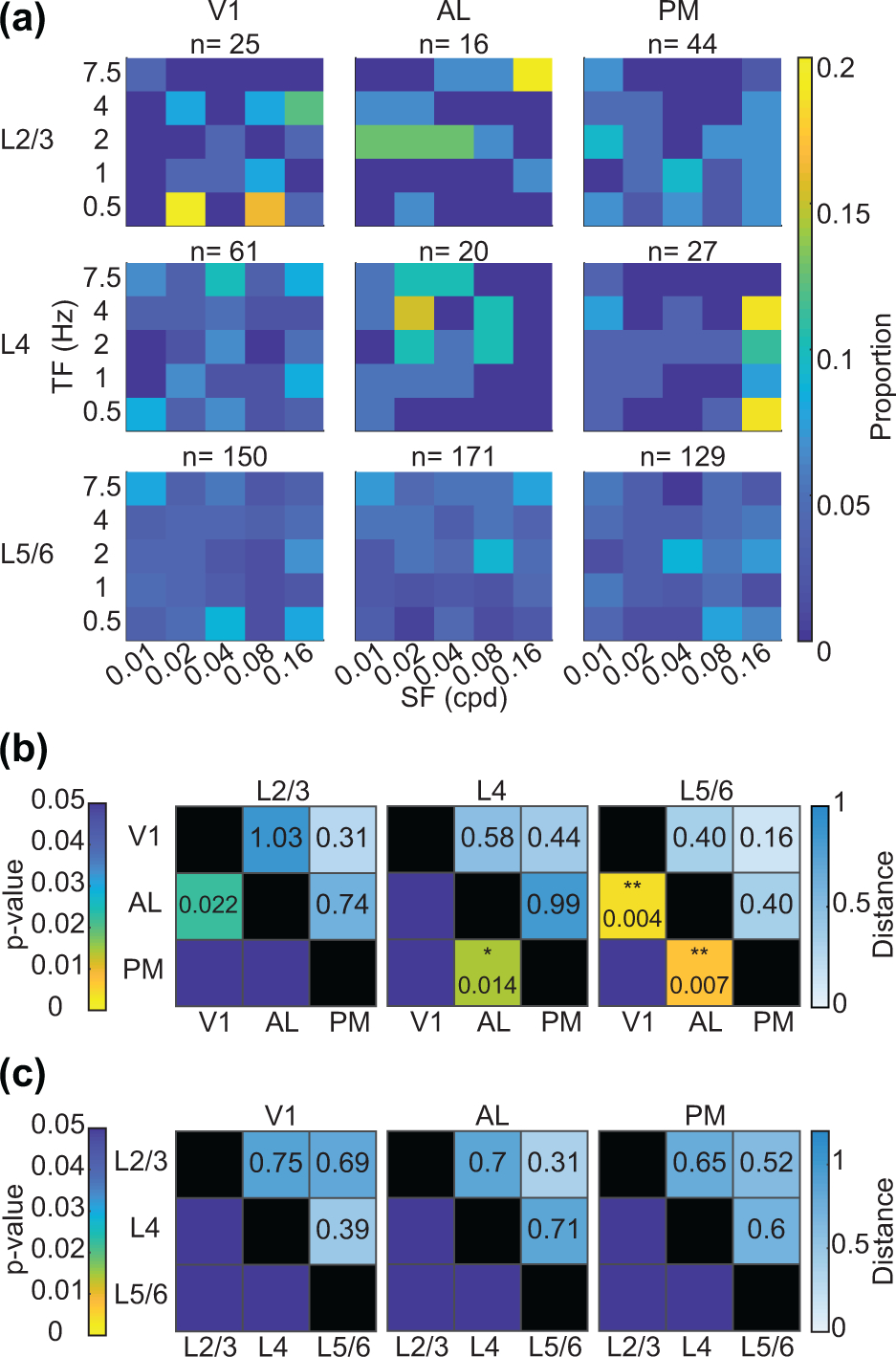
Multivariate analysis of spatiotemporal frequency tuning across areas and layers. (a) 2-D histogram of preferred SF and TFs across layers and areas. (b) Mahalanobis generalized distances between visual areas by layer assignment. Upper triangle numbers indicate distances. Lower triangle stars and numbers indicate p-values. *p<0.016, **p<0.01, and ***p<0.001 (F-statistic with Bonferroni correction for multiple comparisons (p<0.05/3)). P-values are listed for values <0.05. (c) Same as (b), but the Mahalanobis generalized distance between layers by visual areas. Abbreviations: cpd = cycles per degree.

Estimation of speed tuning by 2-D Gaussian fitting reveals few speed tuned neurons

Neurons that are speed tuned do not prefer a single SF or TF, but instead prefer a ratio of TF/SF (speed) across different SFs and TFs. When plotted in log₂ scale, this results in a “ridge” of preferred responses that falls along a line with a slope approximately equal to 1 (Priebe et al., 2003, 2006). Thus, neurons that are speed tuned are more likely to have a speed tuning slope near 1, whereas neurons that are not speed tuned will not. Previous studies in mice have found few speed tuned neurons in V1, but more speed tuned neurons in area PM (Andermann et al., 2011; Ledue et al., 2012; Salinas et al., 2021). To estimate speed tuning and preferred speed of speed tuned neurons we fitted the responses of each neuron to different SFs and TFs to a modified 2-D Gaussian (Figure 7a,b) (see Materials and Methods). We found AL to be significantly more speed tuned compared to V1 and PM (Figure 7a, V1 p =2.60e-6 and PM p= 0.004, Table 1) and AL to have a higher proportion of speed tuned neurons (Figure 7c).

Figure 7:

Speed tuning of V1, AL, and PM neurons. (a) Histograms of speed tuning slopes for neurons significantly speed tuned versus not speed tuned. Lighter color corresponds to non-speed tuned neurons, and darker color corresponds to speed tuned neurons. Statistical comparisons are for differences in the distribution of speed tuning slopes. (b) Preferred speed of speed tuned neurons. For both (a) and (b), *p<0.05; **p<0.01; ***p<0.001 (Kruskal-Wallis followed by Dunn’s post hoc test and Šidàk multiple comparisons). P-values are listed for values <0.05. Filled triangles correspond to the median, and open triangles correspond to the mean of each distribution. (c) Proportion of neurons across all layers that were speed tuned versus not speed tuned.

Range of visual stimulus sampling space can shift area tuning preferences

Recently, the Allen Brain Observatory published a large extracellular electrophysiology data set which includes tuning responses to visual stimuli for neurons across several mouse cortical and subcortical visual areas (Dataset:Allen Institute MindScope Program, 2019; Siegle et al., 2021a). While SF and TF tuning preferences were also examined in this study, their stimulus set differed from ours in that more directions were sampled (8 versus 2–4), SF tuning was measured using whole field static gratings, and TF tuning preferences were measured at a single SF (SF = 0.04 cpd). Because the preferred TF can depend on the SF of the grating and vice-versa (Priebe et al., 2006), we compared the distribution of preferred TF that we found in our study to the preferred TF found in the Allen Visual Coding dataset. We found that when we subsampled our TF tuning data to match the Allen TF tuning stimulus set and only include trials with SF= 0.04 cpd, the preferred TF shifted towards lower TFs (Figure 8a–b) and closer to the distribution of preferred tuning from the Visual Coding dataset (Figure 8c p = 0.022). No significant differences between our TF tuning distributions or our subsampled TF tuning distributions were found compared to the Visual Coding TF tuning distributions.

Figure 8:

Effect of spatial frequency sampling on preferred temporal frequency tuning. (a)-(c) Preferred TF for V1, AL and PM, where (a) the preferred TF is taken from all visually responsive neurons sampled at the preferred SF, (b) preferred TF taken from all visually responsive neurons sampled with SF = 0.04 cpd only, and (c) preferred TF from visually responsive units from Allen Visual Coding, temporal frequency tuning experiments (in those experiments only SF=0.04 cpd was sampled). Note that our TF sampling range differed by one octave compared to the Allen Visual Coding dataset (Dataset:Allen Institute MindScope Program, 2019; Siegle et al., 2021a). *p<0.05; **p<0.01; ***p<0.001 (Kruskal-Wallis followed by Dunn’s post hoc test and Šidàk multiple comparisons). Statistical comparisons were done after rebinning both data sets to have matching TF sampling ranges (1–7.5 Hz). Filled triangles correspond to the median, and open triangles correspond to the mean of each distribution. Abbreviations: cpd = cycles per degrees.

2PCI of two layer 5 neuronal classes reveals area and cell-class differences in SF, TF tuning preferences

Because there are multiple excitatory cell types in different cortical layers that cannot be distinguished by extracellular electrophysiology, we also used transgenic mouse lines with 2PCI to selectively characterize different, identified cell classes in layer 5. We used two mouse lines that label either ET (Npr3-Cre-NEO-IRES) or IT (Tlx3-Cre) projecting layer 5 excitatory neurons (Gerfen et al., 2013; Daigle et al., 2018). The selectivity of these mouse lines for labeling layer 5 ET or IT neurons has been well characterized by previous studies from our lab (Kim et al., 2015; Kirchgessner et al., 2021). Although we did not note differences in tuning preferences between L5ET versus L5IT neurons in any areas for SF, TF or TF/SF, differences between areas were present for each cell class. Between regions, we found that both L5IT and L5ET neurons were tuned differently for SF and TF/SF. These differences were primarily between AL-PM (SF L5IT p= 2.04e-4, and L5ET p=0.002; TF/SF L5ET p= 6.70e-5) and AL-V1 (Figure 9a, SF L5IT p=5.83e-4 and L5ET p=7.89e-6; TF/SF L5IT p=5.53e-13, and L5ET p=1.98e-7). In agreement with past studies, AL neurons preferred lower SFs, and faster TF/SF ratios compared to V1 and PM (Figure 9a). While L5IT neurons in AL preferred higher TFs compared to V1 and PM (Figure 9a, AL-V1 p=1.23e-10 and AL-PM p= 0.001), no differences in TF preferences were found for L5ET neurons. We also did not find significant differences in tuning between V1-PM for either cell class. While we did not observe any statistically significant differences in SF, TF tuning between the layer 5 cell classes, there was a trend in V1 for L5ET neurons to prefer higher TFs and lower SFs than L5IT neurons (TF p = 0.035, SF p=0.013, Table 7).

Figure 9:

Differences in spatiotemporal frequency tuning preferences between L5ET and L5IT populations and across V1, AL and PM. (a) L5IT (Tlx3) versus L5ET (Npr3) SF, TF, and TF/SF histograms (left to right). *p<0.05; **p<0.01; ***p<0.001 (for across area comparisons-Kruskal-Wallis followed by Dunn’s post hoc test and Šidàk multiple comparisons, for between mouse line comparisons-Wilcoxon Rank-Sum test). P-values listed for values < 0.05. Filled triangles correspond to the median, and open triangles correspond to the mean of each distribution. (b) Averaged z-scored responses of responsive neurons in V1, AL, and PM to SFs and TFs sampled at each neuron’s preferred direction. Top row corresponds to L5IT, bottom row corresponds to L5ET. Abbreviations: cpd = cycles per degree, °/s = degrees per second.

When plotting the average z-scored responses (Figure 9b) and distribution of preferred SF and TF together in 2-D histograms (Figure 10a), we found that for L5IT and L5ET neurons, there was a wide range of combinations of SFs and TFs that neurons could prefer, similar to our histograms from electrophysiology recordings of deep layer neurons (Figure 6a). However, certain combinations were more strongly preferred in different regions and mouse lines, so we again calculated the Mahalanobis generalized distances between cells for each region and mouse’s distributions. We found differences largely consistent with our analysis of SF, TF, and TF/SF alone, with differences found between V1-AL (L5IT p=7.9e-14 and L5ET p=3.7e-7) and AL-PM (L5IT p= 5.6e-7 and L5ET p=2.4e-4) for both L5IT and L5ET neurons (Figure 10b).

Figure 10:

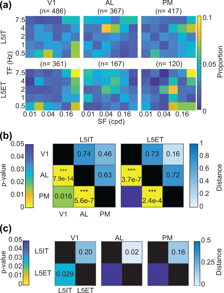
Multivariate analysis of SF, TF responses. (a) 2D histogram of preferred SFs and TFs for each mouse line and region. (b) Mahalanobis generalized distances between regions per mouse line. Upper triangle numbers indicate distances. Lower triangle stars and numbers indicate p-values. *p<0.016, **p<0.01, and ***p<0.001 (F-statistic with Bonferroni correction for multiple comparisons (p<0.05/3)). P-values are listed for values <0.05. (c) Same as (b) but the Mahalanobis generalized distances between each mouse line per region. Abbreviations: cpd = cycles per degree.

Layer 5 neurons are more speed tuned in higher visual areas, but speed tuning does not differ between layer 5 cell classes

We also used our fitted data set to compare speed tuning index and preferred speed of speed tuned neurons across AL, PM and V1 and between L5IT and L5ET neurons. Between regions, we found that both IT and ET neurons in PM were more speed tuned compared to V1 (Figure 11a, L5IT p = 1.91e-4; L5ET p = 4.74e-6). PM L5ET neurons were also more speed tuned than their counterparts in AL (Figure 11a, p=0.017). Between L5IT and L5ET neurons, PM L5ET neurons were more speed tuned compared to PM L5IT neurons (Figure 11a, p= 0.004). Preferred speed did not differ between cell classes and only differed across regions for IT neurons, with AL speed tuned neurons preferring faster speeds compared to V1 and PM (Figure 11b, V1 p= 0.002 and PM p = 2.96e-4). The proportion of neurons that were classified as speed tuned was similar between ET and IT neurons, but differed across areas, with AL and PM both having a higher proportion of speed tuned neurons compared to V1 (Figure 11c). Taken together, higher visual areas tended to be more speed tuned compared to V1. L5ET PM neurons were especially speed tuned compared to other L5ET neurons in AL, as well as compared to L5IT neurons in PM.

Figure 11:

Speed tuning properties of layer 5 ET versus IT cell classes across V1, AL and PM. (a) Speed tuning slope distribution across regions and layer 5 cell classes. (b) Preferred speed distribution across regions and layer 5 cell classes. For both (a) and (b), *p<0.05; **p<0.01; ***p<0.001 (for across area comparisons-Kruskal-Wallis followed by Dunn’s post hoc test and Šidàk multiple comparisons, for between mouse line comparisons- Wilcoxon Rank-Sum test). P-values listed for values <0.05. Filled triangles correspond to the median, and open triangles correspond to the mean of each distribution. (c) Proportion of neurons that were speed tuned versus not speed tuned across areas for each mouse line.

Layer 5 cell classes differ in their direction selectivity in V1, AL, and PM

We also compared orientation and direction tuning between L5IT and L5ET cells since previous studies found differences in orientation and direction selectivity between different layer 5 cell classes in V1 (Kim et al., 2015). Because it would not have been possible to reasonably sample the full SF, TF and direction space all at once, we measured direction and orientation tuning with a separate set of gratings that drifted in 8 directions at either 1 or 2 different SF and TF combinations (Figure 12a). We found that most differences were between cell classes and their direction selectivity. L5ET neurons were more direction selective than L5IT neurons not only in V1, but also in higher visual areas AL and PM (Figure 12c, V1 p = 4.77e-6, AL p = 9.90e-5, and PM p = 4.25e-6).

Figure 12:

Orientation and direction selectivity differences between regions and layer 5 cell types. (a) Sample direction tuning curves from V1, AL, and PM for L5IT and L5ET neurons (top and bottom). For AL and PM, different colored tuning curves correspond to two different SF, TF combinations presented. Thicker line corresponds to mean response at each direction, and shading corresponds to the standard error (sem). (b) Orientation selectivity index (OSI) and (c) Direction selectivity index (DSI). *p<0.05; **p<0.01; ***p<0.001 (for across area comparisons- Kruskal-Wallis followed by Dunn’s post hoc test and Šidàk multiple comparisons, for between mouse line comparisons- Wilcoxon Rank-Sum test). P-values listed for values <0.05. Filled triangles correspond to the median, and open triangles correspond to the mean of each distribution.

Discussion

We used two common methods for recording neural activity, extracellular electrophysiology and 2PCI to create an extensive dataset examining the specialization of V1, AL, and PM in the mouse visual system to SF and TF tuning. In contrast to previous studies, we used laminar probes and imaging to focus our attention to deeper layer cortical neurons, whose tuning have not been as well characterized as superficial cortical neurons in the past. We found that deep versus superficial neurons are largely specialized in similar ways in different cortical areas, consistent with past studies that have focused on superficial layers. We were surprised, however, at the variety of overlapping tuning preferences for SF and TF that we found in our experiments comparing AL and PM. Additionally, we characterized the orientation and direction tuning properties of layer 5 ET and IT projecting neurons in AL and PM and revealed differences between layer 5 ET and IT neurons in these higher visual areas for these visual features.

Functional specialization of mouse higher visual areas

Since early studies characterizing the visual response properties of mouse V1 and HVAs (Andermann et al., 2011; Marshel et al., 2011), AL and PM have often been studied as opposing areas with “fast” versus “slow” visual stimuli preferences. These differences in tuning have been used to understand how specialization may emerge from targeted V1 projections versus other sources, such as de-novo computations or non-V1 inputs (Glickfeld et al., 2013; Kim et al., 2020; Blot et al., 2021). In agreement with these functional biases, it has been demonstrated that AL versus PM projecting V1 neurons rarely connect with each other in V1, differ in gene expression, and usually project to one or the other and rarely to both areas (Kim et al., 2018, 2020). However, the results from our study suggest that, while biases in AL and PM tuning exist for different SFs and TFs, there is also extensive overlap in range of SFs and TFs that neurons in these areas prefer, suggesting less functional specialization than previous studies (Figure 5, Figure 9).

The exact role each HVA plays in processing visual information remains to be elucidated, and likely is not as simple as a segregation of fast versus slow moving stimuli or tasks. Recent studies have demonstrated different roles for some of these areas in visually guided behavioral tasks (Jin and Glickfeld, 2020). Yet, these differences have not always come down to simply differences in visual perception. In Jin and Glickfeld 2020, PM was found to affect false alarm rates during a contrast change detection task and speed increment detection task, but suppression of PM did not affect sensory perception itself (Jin and Glickfeld, 2020). Additional types of visual stimuli or visually guided tasks may be necessary to tease apart how HVAs and their responses relate to their role in mouse visual processing.

Speed tuning in primates is thought to emerge either in V1 or MT (Priebe et al., 2003, 2006). To create speed tuning, spatiotemporal energy models propose that speed tuned units combine inputs from non-speed tuned neurons that prefer different SFs, and TFs, but have the same TF/SF ratio, or speed (Adelson and Bergen, 1985). In mice, few neurons were speed tuned, but we found that HVAs were more speed tuned than V1 (Figure 7, 11). In contrast with previous mouse studies finding more speed tuning only in PM (Andermann et al., 2011), we found that AL was also more speed tuned compared to V1 (Andermann et al., 2011). This difference might be due to preferential sampling of superficial layers (Andermann et al., 2011) versus deep layers (our study). But the difference is unlikely to arise from differential sampling using electrophysiology versus 2PCI since we found AL to have a greater proportion of speed tuned neurons in both datasets (however, AL did not have a statistically significant greater speed tuning slope in the 2PCI data).

Unlike past studies, our study was biased towards sampling deeper layer cortical neurons in awake mice using stationary trials. While decreased sampling of superficial layers made it difficult to draw statistically significant conclusions, we noticed a trend where superficial units seemed more specialized for distinct SF and TF combinations compared to the deeper layers (Figure 6a). Thus, some of the overlap we found between AL and PM tuning preferences for SF and TF may be due to differences in layer 2/3 versus layer 5/6 cells. Layer 2/3 and layer 5/6 neurons play distinct roles in the canonical cortical microcircuit, and thus may differ in their visual responses based on their specific feedforward or feedback roles. Some HVAs receive more V1 input from superficial layer neurons, whereas others receive more input from deeper layer inputs (Kim et al., 2018, 2020). While neurons across cortical depths project to both superficial and deep layers of their cortical targets, different laminar cell types can differ in the laminar pattern of their corticocortical projections (Harris et al., 2019). In addition to different roles in cortico-cortical circuits, some layer 5/6 cell types project extratelencephalically and may play different subcortical roles in visual circuits.

While rodent V1 is traditionally thought to have a “salt and pepper” map of visual tuning preferences (Ohki et al., 2005), studies have suggested that there is a fine-scale modular organization in V1 for some cell types and tuning properties (Ji et al., 2015; Maruoka et al., 2017; D’Souza et al., 2019). In particular, it has been demonstrated in V1 that regions of layer 2/3 that prefer high SFs and low TFs are aligned with “patches” that receive strong cortical feedback and geniculocortical inputs in layer 1 (Ji et al., 2015). In contrast, cells in “interpatches” preferred low SFs, high TFs (Ji et al., 2015). Thus, in addition to cell class and areal differences in SF, TF tuning, there may be within-area tuning differences in sub-domains that are specialized for processing different streams of visual information. It would be interesting in future functional studies to determine if a similar modular pattern for SF, TF tuning is present in other visual areas, and if such an organization is related to specific cell classes.

Stimulus Sampling and Tuning Differences

The extent to which different studies have found differences between V1, AL and PM have varied. While our study primarily differed from previous studies in sampling methodology (extracellular electrophysiology) and depth (deep layer neurons), differences in the behavioral state of the mice between studies may also account for some of the differences observed. For example, in some studies mice were anesthetized with different agents (Marshel et al., 2011 isofluorane; Roth et al., 2012 urethane), while others used awake mice and incorporated both running and stationary trials in their calculations of tuning curves (Andermann et al., 2011). More recently, a study has demonstrated that the selection criteria used to include neurons as “responsive” or not, can also impact the population tuning preferences (Mesa et al., 2021). Differences in visual stimuli, such as whole field versus presentation within a defined aperture, and range of SF, TF sampled may also impact the calculated tuning preferences. This may be especially important for speed tuned neurons where the preferred SF and TF vary depending on each other. In this study, we found that if we subsampled our data to a limited range of SFs, the measured preferred TF shifted to lower TF preferences (Figure 8). Thus, sampling at a non-preferred SF or TF may impact the tuning preferences found in each study.

2PCI versus Extracellular Electrophysiology

2PCI and extracellular electrophysiology using laminar probes are both powerful tools for recording activity from large ensembles of neurons. However, inherent limitations with each technique can limit or bias the types of neurons recorded (Siegle et al., 2021b). While laminar electrophysiological probes in theory allow for unbiased sampling across all cortical depths, we found that superficial single units were often more difficult to isolate and resulted in fewer single-units being sampled. A similar dataset from the Allen Visual Coding dataset using Neuropixel probes also has far fewer superficial cortical units compared to deeper units (Siegle et al., 2021b). Superficial units may be more difficult to sample and isolate with extracellular electrophysiology due to their lower firing rates compared to deep-layer cells (Harris et al., 2016). Despite differences in recording technique and cell types sampled, we found that AL consistently differed from V1 and PM, but V1 and PM did not significantly differ for most tuning properties. However, we did find that, while TF differences were the main driver of differences between AL and other regions in our electrophysiology dataset, the 2PCI data set was more separated by SF differences. While both datasets were biased to deep layers, our electrophysiology data set includes all regular-spiking (putative excitatory) neurons and grouped layer 5 and 6 neurons together as “deep layer” neurons since CSD landmarks cannot reliably separate layers 5 and 6 in HVAs. Since we were unable to exactly match our deep layer electrophysiology and 2PCI populations, the difference in tuning preferences may reflect differences in the deep layer neurons that were sampled with each method.

Layer 5 ET versus IT Populations

In this study, we extended upon previous work examining visual tuning differences between L5ET and L5IT neurons in V1 by also finding differences between L5ET and L5IT populations in HVAs. We find that like superficial neurons, L5ET and L5IT neurons both exhibit functional specializations in AL and PM, with biases towards high versus low TF/SF ratios respectively (Figure 9, 10). However, in contrast with previous papers that recorded superficial V1 and PM neurons and found PM neurons to prefer slower, or similar TFs to V1 and slower TF/SF ratios (Andermann et al., 2011; Roth et al., 2012), we did not observe any significant differences in SF, TF tuning between V1 and PM. This may be potentially attributed to different selection criteria (Mesa et al., 2021), or layer 5 versus layer 2/3 differences.

Overall, we did not find many differences in SF, TF tuning between L5ET versus L5IT neurons. A previous study in V1 found L5ET neurons preferred higher TFs than L5IT neurons (Kim et al., 2015). In our study, we saw a similar trend, but it did not reach statistical significance. However, this could potentially be due to differences in mouse lines used to measure L5IT neurons (Glt25d2-Cre versus Npr3-Cre-NEO) or behavioral state (movement restricted versus freely running on wheel). Expression is much sparser in the Glt25d2-Cre mouse line than Npr3-Cre-NEO. We also characterized speed tuning properties of L5ET and IT neurons and found that PM L5ET neurons were not only more speed tuned than L5ET neurons in other regions, but also more speed tuned compared to their L5IT counterparts (Figure 11). A past study characterizing layer 5 neurons in V1 also noted more direction selectivity in V1 L5ET neurons than V1 L5IT neurons, and we were intrigued to see that this difference persists in HVAs (Kim et al., 2015) (Figure 12).

While we did not find differences in SF, TF or orientation tuning between L5ET and L5IT neurons, there may be additional cell types that we did not discriminate between. For example, feedback IT neurons may be more specialized in HVAs compared to non-feedback IT neurons (Huh et al., 2018). Additionally, L5ET neurons project to several target regions, including superior colliculus, thalamus, striatum, and pons, and a single ET neuron may project to more than one of these targets (Kirchgessner et al., 2021; Zhang et al., 2021). In V1, corticotectal and corticostriatal neurons have been demonstrated to exhibit differences in contrast sensitivity and tuning selectivity for orientation and SF (Lur et al., 2016). V1 ET neurons that project to striatum versus pons have also been demonstrated to play different roles in an eyeblink conditioning task (Tang and Higley, 2020). However, corticostriatal neurons consist of both ET and IT neurons, so differences in these studies between corticostriatal versus other projection targets may also be related to ET versus IT differences (Baker et al., 2018).

Overall, we have conducted an extensive overview of SF, TF, orientation and direction tuning properties of mouse deep layer visual cortical neurons that adds valuable data to the rich literature that currently exists for superficial mouse visual cortical neurons. While our data show many consistencies across superficial and deep layers, we also revealed key cell class differences between different projection populations in higher visual areas, particularly for direction selectivity and speed tuning. Additional studies that more clearly separate cell classes or probe functional specialization using novel stimulus sets or visually-guided behaviors may provide useful further clarification on how cell types across the visual cortex differentially process and use visual information.

Table 6: 2PCI comparisons between regions per L5 cell type.

All statistical comparisons between regions for each L5 cell class. Bolded black p-values are comparisons significant both with the by cell analysis and the hierarchical bootstrap. Non-bold red p-values are comparisons that are significant by cell, but not by hierarchical bootstrap. Bold red p-values are comparisons that are significant by hierarchical bootstrap, but not by cell. Non-bold black p-values are comparisons that did not reach significance for both methods. For Kruskal-Wallis followed by Dunn’s post hoc test and Šidàk multiple comparisons, significance set at p<0.05. For hierarchical bootstrap, significance set at p<0.025.

		Multiple Comparisons			Hierarchical Bootstrap
Test Variable	Kruskal-Wallis	AL vs. V1	AL vs. PM	PM vs. V1	AL vs. V1	AL vs. PM	PM vs. V1
L5IT TF	3.44E-10	1.23E-10	0.001	0.007	1.40E-04	0.013	0.068
L5IT SF	6.64E-05	5.83E-04	2.04E-04	0.968	0.002	0.002	0.422
L5IT TF/SF	1.73E-13	5.53E-13	1.54E-08	0.436	0.005	0.052	0.122
L5ET TF	0.014	0.021	0.049	0.983	0.130	0.042	0.279
L5ET SF	9.72E-06	7.89E-06	0.002	0.979	5.00E-06	0.007	0.222
L5ET TF/SF	1.28E-07	1.98E-07	6.70E-05	1.000	1.00E-05	7.29E-04	0.393
L5IT xi	1.73E-04	0.013	0.524	1.91E-04	0.105	0.286	0.037
L5ET xi	4.91E-06	0.043	0.017	4.74E-06	0.059	0.014	3.18E-04
L5IT speed	9.93E-05	0.002	2.96E-04	0.999	0.021	0.005	0.281
L5ET speed	0.324	-	-	-	0.051	0.112	0.367
L5IT OSI	0.087	-	-	-	0.279	0.485	0.306
L5ET OSI	0.053	-	-	-	0.246	0.048	0.287
L5IT DSI	0.028	0.203	0.762	0.025	0.175	0.400	0.086
L5ET DSI	0.089	-	-	-	0.136	0.223	0.490

Data Availability

Data generated by the authors for this study are available from the corresponding author upon reasonable request.

References

- Adelson EH, Bergen JR. 1985. Spatiotemporal energy models for the perception of motion. J Opt Soc Am A 2. [DOI] [PubMed] [Google Scholar]
- Andermann ML, Kerlin AM, Roumis DK, Glickfeld LL, Reid RC. 2011. Functional specialization of mouse higher visual cortical areas. Neuron [Internet] 72:1025–1039. Available from: 10.1016/j.neuron.2011.11.013 [DOI] [PMC free article] [PubMed] [Google Scholar]
- Baker A, Kalmbach B, Morishima M, Kim J, Juavinett A, Li N, Dembrow N. 2018. Specialized subpopulations of deep-layer pyramidal neurons in the neocortex: Bridging cellular properties to functional consequences. J Neurosci [Internet] 38:5441–5455. Available from: http://ml-neuronbrowser.janelia.org/ [DOI] [PMC free article] [PubMed] [Google Scholar]
- Blot A, Roth MM, Gasler I, Javadzadeh M, Imhof F, Hofer SB. 2021. Visual intracortical and transthalamic pathways carry distinct information to cortical areas. Neuron [Internet] 109:1996–2008.e6. Available from: https://linkinghub.elsevier.com/retrieve/pii/S089662732100283X [DOI] [PMC free article] [PubMed] [Google Scholar]
- Daigle TL, Madisen L, Hage TA, Valley MT, Knoblich U, Larsen RS, Takeno MM, Huang L, Gu H, Larsen R, Mills M, Bosma-Moody A, Siverts LA, Walker M, Graybuck LT, Yao Z, Fong O, Nguyen TN, Garren E, Lenz GH, Chavarha M, Pendergraft J, Harrington J, Hirokawa KE, Harris JA, Nicovich PR, McGraw MJ, Ollerenshaw DR, Smith KA, Baker CA, Ting JT, Sunkin SM, Lecoq J, Lin MZ, Boyden ES, Murphy GJ, da Costa NM, Waters J, Li L, Tasic B, Zeng H. 2018. A Suite of Transgenic Driver and Reporter Mouse Lines with Enhanced Brain-Cell-Type Targeting and Functionality. Cell 174:465–480.e22. [DOI] [PMC free article] [PubMed] [Google Scholar]
- Dataset:Allen Institute MindScope Program. 2019. Dataset: Allen Institute MindScope Program. Available from: brain-map.org/explore/circuits
- DeNardo LA, Berns DS, DeLoach K, Luo L. 2015. Connectivity of mouse somatosensory and prefrontal cortex examined with trans-synaptic tracing. Nat Neurosci [Internet] 18:1687–1697. Available from: http://www.nature.com/articles/nn.4131 [DOI] [PMC free article] [PubMed] [Google Scholar]
- D’Souza RD, Bista P, Meier AM, Ji W, Burkhalter A. 2019. Spatial Clustering of Inhibition in Mouse Primary Visual Cortex. Neuron [Internet] 104:588–600.e5. Available from: https://linkinghub.elsevier.com/retrieve/pii/S0896627319307937 [DOI] [PMC free article] [PubMed] [Google Scholar]
- Du J, Blanche TJ, Harrison RR, Lester HA, Masmanidis SC. 2011. Multiplexed, High Density Electrophysiology with Nanofabricated Neural Probes. PLoS ONE [Internet] 6:e26204. Available from: 10.1371/journal.pone.0026204 [DOI] [PMC free article] [PubMed] [Google Scholar]
- Garrett ME, Nauhaus I, Marshel JH, Callaway EM. 2014. Topography and Areal Organization of Mouse Visual Cortex. J Neurosci [Internet] 34:12587–12600. Available from: 10.1523/JNEUROSCI.1124-14.2014 [DOI] [PMC free article] [PubMed] [Google Scholar]
- Gerfen CR, Paletzki R, Heintz N. 2013. GENSAT BAC Cre-Recombinase Driver Lines to Study the Functional Organization of Cerebral Cortical and Basal Ganglia Circuits. Neuron [Internet] 80:1368–1383. Available from: https://linkinghub.elsevier.com/retrieve/pii/S0896627313009197 [DOI] [PMC free article] [PubMed] [Google Scholar]
- Glickfeld LL, Andermann ML, Bonin V, Reid RC. 2013. Cortico-cortical projections in mouse visual cortex are functionally target specific. Nat Neurosci [Internet] 16:219–226. Available from: 10.1038/nn.3300 [DOI] [PMC free article] [PubMed] [Google Scholar]
- Glickfeld LL, Olsen SR. 2017. Higher-Order Areas of the Mouse Visual Cortex. Annu Rev Vis Sci [Internet] 3:251–73. Available from: 10.1146/annurev-vision-102016- [DOI] [PubMed] [Google Scholar]
- Harris JA, Mihalas S, Hirokawa KE, Whitesell JD, Choi H, Bernard A, Bohn P, Caldejon S, Casal L, Cho A, Feiner A, Feng D, Gaudreault N, Gerfen CR, Graddis N, Groblewski PA, Henry AM, Ho A, Howard R, Knox JE, Kuan L, Kuang X, Lecoq J, Lesnar P, Li Y, Luviano J, Mcconoughey S, Mortrud MT, Naeemi M, Ng L, Oh SW, Ouellette B, Shen E, Sorensen SA, Wakeman W, Wang Q, Wang Y, Williford A, Phillips JW, Jones AR, Koch C, Zeng H. 2019. Hierarchical organization of cortical and thalamic connectivity. Nature [Internet] 575:195–202. Available from: 10.1038/s41586-019-1716-z [DOI] [PMC free article] [PubMed] [Google Scholar]
- Harris KD, Quiroga RQ, Freeman J, Smith SL. 2016. Improving data quality in neuronal population recordings. Nat Neurosci [Internet] 19:1165–1174. Available from: http://www.nature.com/articles/nn.4365 [DOI] [PMC free article] [PubMed] [Google Scholar]
- Huh CY, Peach JP, Bennett C, Vega RM, Hestrin S. 2018. Feature-Specific Organization of Feedback Pathways in Mouse Visual Cortex. Curr Biol 28:114–120.e5. [DOI] [PMC free article] [PubMed] [Google Scholar]
- Ji W, Gămănuţ R, Bista P, D’Souza RD, Wang Q, Burkhalter A. 2015. Modularity in the Organization of Mouse Primary Visual Cortex. Neuron [Internet] 87:632–43. Available from: 10.1016/j.neuron.2015.07.004 [DOI] [PMC free article] [PubMed] [Google Scholar]
- Jin M, Glickfeld LL. 2020. Mouse Higher Visual Areas Provide Both Distributed and Specialized Contributions to Visually Guided Behaviors. Curr Biol [Internet] 30:4682–4692.e7. Available from: https://linkinghub.elsevier.com/retrieve/pii/S0960982220313464 [DOI] [PMC free article] [PubMed] [Google Scholar]
- Juavinett AL, Nauhaus I, Garrett ME, Zhuang J, Callaway EM. 2016. Automated identification of mouse visual areas with intrinsic signal imaging. Nat Protoc [Internet] 12:32–43. Available from: 10.1038/nprot.2016.158 [DOI] [PMC free article] [PubMed] [Google Scholar]
- Kerlin AM, Andermann ML, Berezovskii VK, Reid RC. 2010. Broadly Tuned Response Properties of Diverse Inhibitory Neuron Subtypes in Mouse Visual Cortex. Neuron 67:858–871. [DOI] [PMC free article] [PubMed] [Google Scholar]
- Kim EJ, Juavinett AL, Kyubwa EM, Jacobs MW, Callaway EM. 2015. Three Types of Cortical Layer 5 Neurons That Differ in Brain-wide Connectivity and Function. Neuron [Internet] 88:1253–1267. Available from: 10.1016/j.neuron.2015.11.002 [DOI] [PMC free article] [PubMed] [Google Scholar]
- Kim EJ, Zhang Z, Huang L, Ito-Cole T, Jacobs MW, Juavinett AL, Senturk G, Hu M, Ku M, Ecker JR, Callaway EM. 2020. Extraction of Distinct Neuronal Cell Types from within a Genetically Continuous Population. Neuron 107:274–282.e6. [DOI] [PMC free article] [PubMed] [Google Scholar]
- Kim MH, Znamenskiy P, Iacaruso MF, Mrsic-Flogel TD. 2018. Segregated Subnetworks of Intracortical Projection Neurons in Primary Visual Cortex. Neuron [Internet] 100:1313–1321.e6. Available from: 10.1016/j.neuron.2018.10.023 [DOI] [PubMed] [Google Scholar]
- Kirchgessner MA, Franklin AD, Callaway EM. 2021. Distinct “driving” versus “modulatory” influences of different visual corticothalamic pathways. Curr Biol [Internet]:S0960982221012653. Available from: https://linkinghub.elsevier.com/retrieve/pii/S0960982221012653 [DOI] [PMC free article] [PubMed] [Google Scholar]
- Ledue EE, Zou MY, Crowder NA. 2012. Spatiotemporal tuning in mouse primary visual cortex. Neurosci Lett 528:165–169. [DOI] [PubMed] [Google Scholar]
- Legendre P, Legendre L. 1998. Ecological resemblance. In: Numerical Ecology. Vol. 20. Developments in Environmental Modelling. Elsevier. p 247–302. Available from: https://linkinghub.elsevier.com/retrieve/pii/S0167889298800596 [Google Scholar]
- Li JY, Hass CA, Matthews I, Kristl AC, Glickfeld LL. 2020. Distinct recruitment of feed-forward and recurrent pathways across higher-order areas of mouse visual cortex. Neuroscience. Available from: 10.1101/2020.09.24.312140 [DOI] [PMC free article] [PubMed] [Google Scholar]
- Lur G, Vinck MA, Tang L, Cardin JA, Higley MJ. 2016. Projection-Specific Visual Feature Encoding by Layer 5 Cortical Subnetworks. Cell Rep [Internet] 14:2538–2545. Available from: 10.1016/j.celrep.2016.02.050 [DOI] [PMC free article] [PubMed] [Google Scholar]
- Lyon DC, Nassi JJ, Callaway EM. 2010. A Disynaptic Relay from Superior Colliculus to Dorsal Stream Visual Cortex in Macaque Monkey. Neuron [Internet] 65:270–279. Available from: https://linkinghub.elsevier.com/retrieve/pii/S0896627310000085 [DOI] [PMC free article] [PubMed] [Google Scholar]
- Marshel JH, Garrett ME, Nauhaus I, Callaway EM. 2011. Functional specialization of seven mouse visual cortical areas. Neuron [Internet] 72:1040–1054. Available from: 10.1016/j.neuron.2011.12.004 [DOI] [PMC free article] [PubMed] [Google Scholar]
- Maruoka H, Nakagawa N, Tsuruno S, Sakai S, Yoneda T, Hosoya T. 2017. Lattice system of functionally distinct cell types in the neocortex. Science [Internet] 358:610–615. Available from: 10.1126/science.aam6125 [DOI] [PubMed] [Google Scholar]
- Mesa N, Waters J, de Vries SEJ. 2021. The effect of inclusion criteria on the functional properties reported in mouse visual cortex. eNeuro [Internet] 8:1–9. Available from: 10.1523/ENEURO.0188-20.2021 [DOI] [PMC free article] [PubMed] [Google Scholar]
- Mishkin M, Ungerleider LG, Macko KA. 1983. Object vision and spatial vision: two cortical pathways. Trends Neurosci [Internet] 6:414–417. Available from: https://linkinghub.elsevier.com/retrieve/pii/016622368390190X [Google Scholar]
- Movshon JA. 1975. The velocity tuning of single units in cat striate cortex. J Physiol 249:445–468. [DOI] [PMC free article] [PubMed] [Google Scholar]
- Murakami T, Matsui T, Ohki K. 2017. Functional segregation and development of mouse higher visual areas. J Neurosci [Internet] 37:9424–9437. Available from: https://www.jneurosci.org/content/37/39/9424 [DOI] [PMC free article] [PubMed] [Google Scholar]
- Nassi JJ, Callaway EM. 2009. Parallel processing strategies of the primate visual system. Nat Rev Neurosci [Internet] 10:360–372. Available from: http://www.nature.com/articles/nrn2619 [DOI] [PMC free article] [PubMed] [Google Scholar]
- Niell CM, Stryker MP. 2010. Modulation of Visual Responses by Behavioral State in Mouse Visual Cortex. Neuron [Internet] 65:472–479. Available from: https://linkinghub.elsevier.com/retrieve/pii/S0896627310000590 [DOI] [PMC free article] [PubMed] [Google Scholar]
- Ohki K, Chung S, Ch’ng YH, Kara P, Reid RC. 2005. Functional imaging with cellular resolution reveals precise micro-architecture in visual cortex. Nature [Internet] 433:597–603. Available from: http://www.nature.com/articles/nature03274 [DOI] [PubMed] [Google Scholar]
- Pachitariu M, Steinmetz N, Kadir S, Carandini M, Harris KD. 2016a. Kilosort: realtime spike-sorting for extracellular electrophysiology with hundreds of channels. bioRxiv [Internet]:061481. Available from: 10.1101/061481 [DOI] [Google Scholar]
- Pachitariu M, Stringer C, Schröder S, Dipoppa M, Rossi LF, Carandini M, Harris KD. 2016b. Suite2p: beyond 10,000 neurons with standard two-photon microscopy. bioRxiv [Internet]:061507. Available from: http://biorxiv.org/content/early/2016/06/30/061507 [Google Scholar]
- Pettersen KH, Devor A, Ulbert I, Dale AM, Einevoll GT. 2006. Current-source density estimation based on inversion of electrostatic forward solution: Effects of finite extent of neuronal activity and conductivity discontinuities. J Neurosci Methods [Internet] 154:116–133. Available from: https://linkinghub.elsevier.com/retrieve/pii/S0165027005004541 [DOI] [PubMed] [Google Scholar]
- Priebe NJ, Cassanello CR, Lisberger SG. 2003. The neural representation of speed in macaque area MT/V5. J Neurosci 23:5650–5661. [DOI] [PMC free article] [PubMed] [Google Scholar]
- Priebe NJ, Lisberger SG, Movshon JA. 2006. Tuning for Spatiotemporal Frequency and Speed in Directionally Selective Neurons of Macaque Striate Cortex. J Neurosci [Internet] 26:2941–2950. Available from: 10.1523/JNEUROSCI.3936-05.2006 [DOI] [PMC free article] [PubMed] [Google Scholar]
- Roth MM, Helmchen F, Kampa BM. 2012. Distinct Functional Properties of Primary and Posteromedial Visual Area of Mouse Neocortex. J Neurosci [Internet] 32:9716–9726. Available from: 10.1523/JNEUROSCI.0110-12.2012 [DOI] [PMC free article] [PubMed] [Google Scholar]
- Salinas KJ, Huh CYL, Zeitoun JH, Gandhi SP. 2021. Functional Differentiation of Mouse Visual Cortical Areas Depends upon Early Binocular Experience. J Neurosci [Internet] 41:1470–1488. Available from: 10.1523/JNEUROSCI.0548-20.2020 [DOI] [PMC free article] [PubMed] [Google Scholar]
- Saravanan V, Berman GJ, Sober SJ. 2020. Application of the hierarchical bootstrap to multi-level data in neuroscience. Neurons Behav Data Anal Theory [Internet] 3:https://nbdt.scholasticahq.com/article/13927-application-of-the-hierarchical-bootstrap-to-multi-level-data-in-neuroscience. Available from: https://www.ncbi.nlm.nih.gov/pmc/articles/PMC7906290/ [PMC free article] [PubMed] [Google Scholar]
- Schmitzer-Torbert N, Jackson J, Henze D, Harris K, Redish AD. 2005. Quantitative measures of cluster quality for use in extracellular recordings. Neuroscience [Internet] 131:1–11. Available from: https://linkinghub.elsevier.com/retrieve/pii/S0306452204008425 [DOI] [PubMed] [Google Scholar]
- Shobe JL, Claar LD, Parhami S, Bakhurin KI, Masmanidis SC. 2015. Brain activity mapping at multiple scales with silicon microprobes containing 1,024 electrodes. J Neurophysiol [Internet] 114:2043–2052. Available from: 10.1152/jn.00464.2015 [DOI] [PMC free article] [PubMed] [Google Scholar]
- Siegle JH, Jia X, Durand S, Gale S, Bennett C, Graddis N, Heller G, Ramirez TK, Choi H, Luviano JA, Groblewski PA, Ahmed R, Arkhipov A, Bernard A, Billeh YN, Brown D, Buice MA, Cain N, Caldejon S, Casal L, Cho A, Chvilicek M, Cox TC, Dai K, Denman DJ, de Vries SEJ, Dietzman R, Esposito L, Farrell C, Feng D, Galbraith J, Garrett M, Gelfand EC, Hancock N, Harris JA, Howard R, Hu B, Hytnen R, Iyer R, Jessett E, Johnson K, Kato I, Kiggins J, Lambert S, Lecoq J, Ledochowitsch P, Lee JH, Leon A, Li Y, Liang E, Long F, Mace K, Melchior J, Millman D, Mollenkopf T, Nayan C, Ng L, Ngo K, Nguyen T, Nicovich PR, North K, Ocker GK, Ollerenshaw D, Oliver M, Pachitariu M, Perkins J, Reding M, Reid D, Robertson M, Ronellenfitch K, Seid S, Slaughterbeck C, Stoecklin M, Sullivan D, Sutton B, Swapp J, Thompson C, Turner K, Wakeman W, Whitesell JD, Williams D, Williford A, Young R, Zeng H, Naylor S, Phillips JW, Reid RC, Mihalas S, Olsen SR, Koch C. 2021a. Survey of spiking in the mouse visual system reveals functional hierarchy. Nature 592:86–92. [DOI] [PMC free article] [PubMed] [Google Scholar]
- Siegle JH, Ledochowitsch P, Jia X, Millman DJ, Ocker GK, Caldejon S, Casal L, Cho A, Denman DJ, Durand S, Groblewski PA, Heller G, Kato I, Kivikas S, Lecoq J, Nayan C, Ngo K, Nicovich PR, North K, Ramirez TK, Swapp J, Waughman X, Williford A, Olsen SR, Koch C, Buice MA, de Vries SE. 2021b. Reconciling functional differences in populations of neurons recorded with two-photon imaging and electrophysiology. eLife [Internet] 10:e69068. Available from: https://elifesciences.org/articles/69068 [DOI] [PMC free article] [PubMed] [Google Scholar]
- Siegle JH, López AC, Patel YA, Abramov K, Ohayon S, Voigts J. 2017. Open Ephys: an open-source, plugin-based platform for multichannel electrophysiology. J Neural Eng [Internet] 14:045003. Available from: http://www.ncbi.nlm.nih.gov/pubmed/28169219 [DOI] [PubMed] [Google Scholar]
- Tang L, Higley MJ. 2020. Layer 5 Circuits in V1 Differentially Control Visuomotor Behavior. Neuron [Internet] 105:346–354.e5. Available from: 10.1016/j.neuron.2019.10.014 [DOI] [PMC free article] [PubMed] [Google Scholar]
- Wang Q, Burkhalter A. 2007. Area map of mouse visual cortex. J Comp Neurol [Internet] 502:339–357. Available from: 10.1002/cne.21286 [DOI] [PubMed] [Google Scholar]
- Zhang Z, Zhou J, Tan P, Pang Y, Rivkin AC, Kirchgessner MA, Williams E, Lee C-T, Liu H, Franklin AD, Miyazaki PA, Bartlett A, Aldridge AI, Vu M, Boggeman L, Fitzpatrick C, Nery JR, Castanon RG, Rashid M, Jacobs MW, Ito-Cole T, O’Connor C, Pinto-Duartec A, Dominguez B, Smith JB, Niu S-Y, Lee K-F, Jin X, Mukamel EA, Behrens MM, Ecker JR, Callaway EM. 2021. Epigenomic diversity of cortical projection neurons in the mouse brain. Nature [Internet] 598:167–173. Available from: https://www.nature.com/articles/s41586-021-03223-w [DOI] [PMC free article] [PubMed] [Google Scholar]
Associated Data
This section collects any data citations, data availability statements, or supplementary materials included in this article.
Data Availability Statement