

Abstract
Forecasting cargo throughput is an essential albeit challenging task in ensuring efficient seaport management. In this study, data analytics is employed to analyze the nonlinear dynamic behaviors, as well as disruptions in port throughputs. Further, nonlinear analytical methods, including the Lyapunov exponent (LE), information entropy, Hurst exponent, and wavelet decomposition, are employed to explore the complex dynamic behavior of port throughput under supply chain disruptions. By employing the discrete wavelet transform (DWT) and the long short-term memory (LSTM) network, we develop a novel hybrid model of port throughput forecasting. DWT is employed to decompose the original data into a finite set of frequency components, so that the various hidden features of cargo throughput can be extracted via different modes, such as the trend, residual, and seasonal components. Thereafter, each component, obtained from the DWT spectra, is predicted via a machine learning model. Additionally, hypothesis testing, model evaluation, and statistical significance tests are employed to comprehensively evaluate the introduced forecasting models. Regarding prediction accuracy and efficiency, our extensive simulation results confirm the superiority of the hybrid strategy over five benchmarked models. Finally, by employing business forecasting software, we show that the robust hybrid strategy achieves accurate predictions of port throughputs against market disruptions. Our findings can help decision-makers understand disruption mechanisms in port systems, thus enabling them to successfully achieve their business goals.
Keywords: Time-series data, Port throughput, Nonlinear dynamic analysis, Discrete wavelet transform, Machine learning, Hybrid forecasting model
Introduction
With the the advent of globalization, ocean transportation, as well as port management, are assuming an essential role in international trade (Notteboom 2016). Cargo throughput is the commonest indicator in evaluating port performance, representing a benchmarking reference for other ports (Justice et al. 2016). Moreover, cargo throughput reflects the economic growth and rigor of a port (Du et al. 2019). However, exploring the underlying mechanisms of cargo throughput development against exogenous and endogenous disruptions is challenging (Gou and Lam 2019). Numerous tools for investigating the dynamic properties of port throughput have been employed in earlier research. These have included nonlinear control theory (Cuong et al. 2021); data envelopment analysis (Tetteh et al. 2016); decomposition-ensemble methodology (Xie et al. 2017) and stochastic modeling (Saini et al. 2017). Although each approach exhibits unique advantages, they do not describe all the typical features of the cargo throughput system in isolation.
The instability of system is induced by multiple shocks, although only a few studies have considered this (Justice et al. 2016). The nonlinear system theory avails an efficient strategy to describe the complex dynamic behavior of a real system (Slotine and Li 1991; Morris and Pratt 2003; Cuong et al. 2021). However, a few empirical studies only have explored the dynamic behavior of cargo throughput systems through nonlinear techniques. The approach employed here can elucidate the underlying mechanisms of cargo throughput systems, helping port policymakers determine appropriate strategies (Zhang and Lam 2017). Additionally, we aim to fill the research gap between the theoretical and practical applications of nonlinear analysis tools, such as the Lyapunov exponent (LE), information entropy, Hurst exponent, and wavelet decomposition, for investigating the dynamic properties of cargo throughput systems under disruptions. Based on the tools discussed here, port decision-makers can gain further insights into nonlinear phenomena, such as periodicity, stability, and chaotic behaviors.
Moreover, port throughput forecasting is crucial to the management, construction, and improvement of port infrastructures, and accurate business forecasting can optimize resource utilization and efficiency, while avoiding investment mistakes (Du et al. 2019; Twrdy and Batista 2016). Conversely, low prediction accuracy, owing to a bias, can cause significant financial losses (Xie et al. 2017). Therefore, a highly effective forecasting method is required for efficient port operations. Additionally, predicting future trends and events leads to informed business decisions.
Autoregressive integrated moving average (ARIMA) forecasting techniques have been widely utilized among practitioners (as a benchmark). Models that have been employed in logistics and supply chain management (Schulze and Prinz 2009) include exponential smoothing (Gosasang et al. 2011), Grey forecasting (Liu and Chen 2006) and deep learning (Yang and Chang 2020; Shankar et al. 2021; Zuo et al. 2021). However, port throughput data reveal complex nonlinear dynamic behaviors under the various disruptions. In such cases, however, Grey forecasting or linear regression do not provide high accuracy, in ever-changing and noisy datasets (Punia et al. 2020).
Recently, deep machine learning has exhibited the promise of AI applications in many forecasting fields, such as multichannel retailers (Ferreira et al. 2016; Punia et al. 2020), financial markets (Fischer and Krauss 2018), and insurance big data analysis (Lin et al. 2017). The advantage of deep learning is in its capacity to create a hybrid function set comprising numerous nonlinear transformations and valuable expressions that can produce additional abstractions, followed by potential benefits (Punia et al. 2020; Hochreiter and Schmidhuber 1997). The convolutional neural network (CNN) is superior to existing methods for image recognition, while the recurrent neural network (RNN) exhibits excellent performance in speech recognition and natural language processing. RNN stores long sequential information in hidden memory for proper processing, representation, and storage (Memarzadeh and Keynia 2020). RNN employing recurrent links between hidden layers has been proposed to process history-related issues in the field of artificial intelligence (AI). Unfortunately, RNN cannot learn long-term historical data, causing an issue that was resolved by Hochreiter and Schmidhuber (1997) via the long short-term memory (LSTM) network, an extension of the RNN algorithm. LSTM can learn the long- and short-term effects of preceding data. LSTM networks with deep architectures have achieved great success in different applications involving large datasets (Zhang et al. 2021; Hochreiter and Schmidhuber 1997).
High-performing powerful algorithms enhance the accuracy of port throughout forecasting during significant economic changes that affect maritime transportation activities, e.g., the 2009 financial crisis or the coronavirus pandemic (COVID-19) (Cullinane and Haralambides 2021). By following existing data-driven solutions to issues of production and operations management (Lin et al. 2017; Fischer and Krauss 2018; Johannesen et al. 2019; Punia et al. 2020; Islam and Amin 2020; Sipper and Moore 2021), this study presents a novel hybrid strategy for addressing complex throughput forecasting scenarios. The proposed algorithm is based on deep learning and employs the LSTM methodology with wavelet decomposition. The effectiveness of our method is assessed via a set of evaluation indices and statistical significance tests. Through effective forecasting, port management can gain valuable insights, reduce costs, increase profitability, learn from mistakes, predict throughput trends, and attain sustainable competitive advantage.
In summary, our novel data analytics methodology is based on time-series analysis, entropy analysis, LE, Hurst exponent, and wavelet decomposition. It can be applied to forecasting issues involving time-series data with market uncertainties caused by multiple disruptive factors. For policymakers, this novel method can offer insights to the system dynamics of port throughput and help them explore the underlying mechanisms of business uncertainties caused by maritime transportation disruptions. Furthermore, our schemes can help port authorities predict the productivity of the port management system, subsequently helping managers to make appropriate operational decisions. Additionally, this study presents an advanced machine learning-based method for improving the accuracies and efficiencies of predictions.
The remainder of this paper is organized as follows: Sect. 2 presents the analysis of port throughput via novel data analytics. Section 3 describes the hybrid forecasting method, and Sect. 4 presents the empirical simulation results, as well as the statistical analysis. Finally, Sect. 5 draws the main conclusions of the study, highlighting the most significant findings.
Data analytics for port throughput
Cargo throughput and maritime traffic volume of Busan Port
To many analysts, the market dynamics of the twenty-first century point out to accelerating globalization and the advent of cross-border economic frictions. In this situation, the hub of global trade and economy is shifting to East Asia, around China. Approximately 50% of global container flows take place in this region, thereby directly and indirectly increasing competition for hub port positions among Asian ports (Lam and Notteboom 2014). Such competition takes place in various fronts, ranging from the production of the port service to attracting transshipment cargo (Dirzka and Acciaro 2021).
Busan Port is located at the mouth of the Naktong River in South Korea. The port is the sixth-busiest port in the world and the largest transshipment center in Northeast Asia (Lee et al. 2021). Data obtained from the port authority show that the port handled 118.74 million tons of transshipment in March 2020, a record high since Busan New Port began operations in 2006. Cargo throughput and ship traffic of the port (during the period of our research, i.e., 2001–2021) are presented in Table 1. Data analytics is vital in getting meaningful insights to time series data. Nonlinear time-series analysis is employed here to systematically explore observed data (typically univariate) and the dynamic behavior of the port management system. The throughput trend was investigated via LE, information entropy, Hurst exponent with fractal dimension, wavelet decomposition, and statistical significance tests.
Table 1.
Cargo throughput and ship traffic at Busan Port (cargo throughput in million tons, including exports, imports and transshipment)
Source Korean Shipping Port Logistics Information System, 2021
| Year | Total | Entry into port | Departure | |||
|---|---|---|---|---|---|---|
| Number of ships | Cargo throughput | Number of ships | Cargo throughput | Number of ships | Cargo throughput | |
| 2001 | 83,547 | 541.14 | 41,779 | 270.40 | 41,768 | 270.74 |
| 2002 | 92,587 | 583.36 | 46,321 | 291.36 | 46,266 | 291.99 |
| 2003 | 94,533 | 626.94 | 47,241 | 313.28 | 47,292 | 313.66 |
| 2004 | 97,329 | 660.36 | 48,671 | 330.07 | 48,658 | 330.29 |
| 2005 | 96,711 | 709.06 | 48,343 | 354.35 | 48,368 | 354.70 |
| 2006 | 100,787 | 728.16 | 50,385 | 363.60 | 50,402 | 364.56 |
| 2007 | 102,852 | 791.10 | 51,395 | 395.13 | 51,457 | 395.97 |
| 2008 | 115,931 | 832.56 | 57,979 | 416.34 | 57,952 | 416.22 |
| 2009 | 100,113 | 852.33 | 50,012 | 425.54 | 50,101 | 426.80 |
| 2010 | 104,995 | 936.42 | 52,484 | 467.81 | 52,511 | 468.61 |
| 2011 | 100,875 | 1027.15 | 50,447 | 513.50 | 50,428 | 513.65 |
| 2012 | 100,845 | 1062.23 | 50,437 | 534.40 | 50,408 | 527.83 |
| 2013 | 99,249 | 1128.25 | 49,588 | 567.88 | 49,661 | 560.37 |
| 2014 | 95,378 | 1107.03 | 47,718 | 557.17 | 47,660 | 549.86 |
| 2015 | 98,087 | 1247.88 | 49,047 | 627.93 | 49,040 | 619.94 |
| 2016 | 100,197 | 1324.57 | 50,089 | 666.04 | 50,108 | 658.53 |
| 2017 | 99,687 | 1332.26 | 49,842 | 669.14 | 49,845 | 663.12 |
| 2018 | 94,816 | 1345.18 | 47,345 | 676.84 | 47,471 | 668.34 |
| 2019 | 93,701 | 1361.34 | 46,834 | 684.98 | 46,867 | 676.36 |
| 2020 | 89,018 | 1324.71 | 44,430 | 665.69 | 44,588 | 659.02 |
| 2021 | 46,704 | 706.16 | 23,186 | 354.58 | 23,518 | 351.58 |
Determination of dynamic behavior via LEs
Graphical methods and quantifiers are commonly employed within the port and logistics research community to identify existing dynamic behaviors, whether a system is stable, periodic, quasiperiodic, or chaotic (Sprott 1995; Hwarng and Xie 2008). Regarding nonlinear time-series analysis, a more accurate alternative, involving the calculation of some quantifiers, can be proposed (Hwarng and Xie 2008). Data analytics is the science of analyzing raw data to offer informed conclusions. Some well-known measures include LE, information entropy, fractal dimension, and capacity dimension (Sprott 1995).
The Lyapunov spectrum facilitates the qualitative and quantitative characterizations of nonlinear features (Wolf et al. 1985). Employing the collected data, LE is obtained by measuring the average exponential rates of divergence or convergence of nearby orbits in phase space. Even though the Lyapunov spectrum can be determined via different approaches, LE is defined in a manner that is most relevant to the spectral calculations from a time series. For a continuous system in n-dimensional phase space, an infinitesimal n-sphere of initial conditions becomes an n-ellipsoid in the long term. Thus, the ith LE index is defined as follows:
| 1 |
where pi(t) is the length of the ellipsoidal principal axis at time t and the λis are typically ordered from the largest to smallest (Wolf et al. 1985). A system is considered to be chaotic if a minimum of one LE or the largest LE (LLE) is positive; otherwise, its dynamic behavior is considered to be stable, periodic, or quasiperiodic (Hwarng and Xie 2008). Chaotic behaviors tend to be very complex in a random manner, although they change according to deterministic rules.
Figure 1 shows the LLE of Busan’s cargo throughput. The application of Wolf et al. (1985) theory reveals that LLE exhibited sequential negative and positive values throughout the development of Busan Port since in 2001. This means that the system exhibits an unstable, complex behavior, tending to be chaotic. These behaviors are caused by transportation disruptions, such as seasonal demand variations and external shocks, particularly the 2009 financial crisis and the COVID-19 pandemic. Moreover, test results showed that LLE fluctuated with a large amplitude at several periods in the time series. Fluctuations during these periods are much larger than those of an average period of the entire system. For example, the value of LLE was − 2.8 at t = 40, compared with the average range of the entire system, which was approximately [-1 2]. Owing to the many uncertainties about the drastic changes in LLE, the existence of large fluctuations requires further clarification. This study offers alternative algorithms, which are more robust than the LE scheme, for identifying specific dynamic behaviors (Clément and Laurens 2011). Furthermore, other alternatives must be explored to verify the dynamic behavior of port throughput under the impact of disruptions.
Fig. 1.

LE spectrum of cargo throughput
Resolving complexity via entropy analysis
Along with LEs, entropic measurement offers a deeper elucidation of the nonlinear features of systems (Jahanshahi et al. 2019). Information entropy is a concept in information theory, employed to measure the complexity and randomness of a time series. The entropy of a dynamic system is determined by the predictability of its dynamic behavior. For example, more-complex systems are less predictable than less complex ones. The Kolmogorov–Sinai entropy is a complicated scheme for computing entropy to measure complexity and randomness from a finite time series. Several methods, such as approximate entropy and sample entropy, have been introduced to address this limitation. However, these approaches have suffered from weak principles (Ye et al. 2020). Contrarily, the permutation entropy (PE, ) represents a robust tool that characterizes the complexity and randomness of a nonlinear time series (Bandt and Pompe, 2002). Our data reveals that the complexity measure is only a function of the probabilities of different states (the computational steps for measuring are summarized in Appendix 1).
Additionally, the measured entropy value, , is always between 0 and 1. Smaller entropy offers more periodicity and regularity in the time series. However, the larger the entropy value, the more irregular and random the time series would be. More specifically, if the time series is white noise, the entropy will be 1. Therefore, PE can be applied to the estimation of the complexity and dynamic changes in the time series. The measures of the complexity in maritime supply chains relate to their manageability and controllability. Thus, complexity reduction might enable port authorities to simplify their strategic goals for business operations against disruptions.
To investigate the stability and disruption of port throughput, the PE method is employed to clarify the dynamic behaviors of throughput trends. The values of training and test samples in the dataset were 197 and 50 data points, respectively, while the sample size, N, was 247. The embedding dimensions and scale factor were set at m = 4 and s = 12, respectively. Figure 2 shows that port throughput can be described by employing the basic properties of information entropy. First, the entropy value is zero at t = 0 because the variable is not random. Next, increases to 0.78 at t = 5 and remains, mostly sideways, for a few subsequent time series before increasing rapidly. From t = 38, PE reaches a value of 1 and maintains that pattern until the end of the period. The test results are employed to describe the historical development of the port, operated by the Busan Port Authority (BPA). Further, internal factors, such as operating procedures, management policies, and constantly changing infrastructure, cause significant fluctuation in cargo throughput trends. Additionally, external shocks, particularly disruptions, such as the 2009 financial crisis and Covid-19, directly disturb the management of port business and operations. Thus, information entropy can be a measure of the degree of systematic ordering or randomness of the time series.
Fig. 2.

Temporal variations of the entropy of cargo traffic (Busan Port)
Next, is employed to investigate the cargo throughput trend for the preceding three years (2018–2020). The test results of the short-term performance are shown in Fig. 3. At the beginning of the test period, the entropy attained low values yearly. Toward the end of the period, it increased significantly and approached in 2020. However, these values were relatively low in 2018 and 2019. Especially, a high entropy value was obtained in 2020 because the port encountered supply chain disruptions in its cargo handling activities, as well as shipping services, owing to the impact of COVID-19; these affected the dynamic behavior of port operations. External shocks have affected cargo throughput, accounting for increasing irregular behaviors. Thus, the entropy value is ~ 1. Concurrently, historical data revealed that the port management system achieved smooth operations during the earlier two years (2018–2019).
Fig. 3.

Comparison of the entropies of Busan Port within 2018–2020
Determining the predictability via HE and fractal dimension
The port management system encounters complex, dynamic, and increasingly challenging disruptive perturbations, such as time delays, regulatory changes, adverse weather, and dynamic interactions between port systems. By employing the introduced approaches, port authorities can identify the quantitative behaviors of nonlinearity, complexity, and chaos of the time series. HE is a robust and efficient tool in exploring the underlying mechanisms, having been applied to time series analysis in finance and logistics research (Corazza and Malliaris 2002; Tzouras et al. 2015; Yao et al. 2014).
HE, proposed by Hurst (1951), is employed in fractal analysis and it is a measure of long-term memory of time-series data. The method can be employed to determine the duration of the impacts of external shocks. The advantages of HE include the simplicity of the basic assumptions, as well as the increased stability of its validity and robustness for numerous types of time series (Corazza and Malliaris 2002). HE (H) is determined via the asymptotic dynamic behavior of the rescaled range as a function of the period (Feder 1988). Employing the collected data, H is calculated via rescaled range analysis (R/S analysis). Regarding the time-series data, , the R/S analysis steps are presented in Appendix 2.
The value of H ranges between 0 and 1, measuring the degree of the deviation of a given time series from a random walk (H = 0.5), with higher values indicating a smoother trend, less volatility, and less roughness. A time series can be classified into the following categories: H = 0.5, representing a random distribution that is indistinguishable from noise or disruption; 0 < H < 0.5, which means that the system exhibits mean-reverting and anti-persistent series behaviors (more chaos); and 0.5 < H < 1.0, which indicates that the system tends to a persistent series (less chaotic or trending). Values near 0 and 1 indicate that the mean-reversion process and trending pattern (the trend will continue) were strong, respectively. The H estimator is a rapid tool for investigating whether the time series is random walking, mean-reverting, or trending.
The complexity of time-series signals was investigated by fractal analysis. Regarding a self-similar time series, H directly relates to the pattern fractal dimension (D), where 1 < D < 2, such that D = 2 − H (Liaw and Chiu 2009). D is a relative measure of the number of elemental units employed to fabricate a pattern. Notably, the rough pattern is represented by a higher D, with a fractal measure ranging from 1 (the dimension along the straight line) to 2 (the dimension of the plane in which the pattern lies). Further, the fractal dimension can also be regarded as an informational measure, which can be employed to directly observe the time series and investigate its nonlinear features. Assuming D = 1.5 (or H = 0.5) obeys a random walk, with any D value other than 1.5, time-series data can be inferred as the absence of randomness.
Figure 4 presents H for a sliding window exhibiting a data length of 147. Overall, it is significantly higher than 0.5 (or D < 1.5) when analyzing the cargo volume of Busan Port, revealing the distinct long-term memory feature in the loading and unloading operations. Results reveal the following information: (1) port throughput is affected by the shipping market and external disruptions, as well as previous and present throughput levels. (2) H is higher than 0.5 under prolonged time series conditions, with many environmental shocks, such as the financial crisis or the pandemic, indicating that the trending pattern was strong on the throughput volume and that the trend will persist (Tzouras et al. 2015; Ye et al. 2020). If the actual cargo volume is lower than the average at a certain point, the throughput will tend to be lower at the subsequent time. Conversely, if the cargo throughput is higher than the average, the cargo volume will tend to increase over time. (3) the port authority could combine the previous interevent time distribution with the present situation and employ analytical and statistical tools to improve management efficiency towards increasing port throughput.
Fig. 4.

H over a sliding window of 145 observations (from May 2009 to July 2021). a R/S ratio; b H
Port productivity analysis using wavelet decomposition
As demonstrated, the cargo throughput of Busan Port is highly volatile, presenting chaotic behavior. As such, forecasting is particularly challenging, for unstable systems are affected by uncertainties and external shocks (Xie et al. 2017). Such predictions cannot be accurate even if they are based on actual numbers. Further, most data are commonly messy or incomplete.
Thus, the wavelet transform is introduced next, to improve forecasting accuracy. So far, this technique has presented a very efficient time-series analysis tool, not very common within the data science community. Wavelet transforms decompose a signal into several sub-signals of different frequency bands. Previous signal-processing techniques, such as the Fourier transform (FT) and short time FT (STFT), exhibit major drawbacks regarding time information and resolution. The utilization of a fully scalable modulated window in the wavelet analysis can solve the above drawbacks. The window or mother wavelet is shifted at every position of the signal, making it possible to calculate the spectrum at each position (Rajaee et al. 2011). There are two basic types of wavelet transformations: the continuous wavelet transform (CWT) and discrete wavelet transform (DWT). CWT is defined in terms of the dilations and translations of a mother wavelet function that can be expressed, as follows (Memarzadeh and Keynia 2020):
| 2 |
where the transformed signal is a function of two variables (‘a’ and ‘b’), which represent the scale and translation parameters, respectively; denotes the complex conjugate of ‘t’ (Mallat 1989); f(t) is the input signal; is the transforming function, which is called the mother wavelet. Since CWT produces N2 coefficients from a dataset of length, N, unnecessary information is hidden within the coefficients (Rajaee et al. 2011). To overcome this limitation, DWT calculates the wavelet coefficients on discrete dyadic scales and time positions, as follows:
| 3 |
where m and n are the integers that regulate the wavelet dilation and translation, respectively; b0 is the location parameter, which must be greater than zero (> 0); a0 is a specified fixed dilation step, which must be greater than one (> 1). The ideal choices of a0 and b0 depend on the wavelet functions. The dyadic wavelet can be written in more compact notation, as follows:
| 4 |
For a discrete time series, xt, the dyadic wavelet transform becomes
| 5 |
where Wm,n is the wavelet coefficient for the discrete wavelet of scale a = 2 m and location b = 2 mn. This formula considers a finite time series, xt, t = 0, 1, 2,…, N-1, and N is an integer power of 2, N = 2 M, and n is the time-translation parameter. This gives the ranges of m and n as 0 < n < 2 M–m–1 and 1 < m < M, respectively. Generally, the time-series patterns of the port throughput exhibit nonlinear and dynamic properties. The trend of the cargo throughput is severely impacted by several factors, such as market changes, shipping costs, and disruptive factors. Next, DWT can be employed to describe the asymmetric nature of this time series. Put differently, DWT can extract the different characteristics of the dataset, such as the low- and high-frequency components.
Here, the Haar wavelet was employed as the wavelet filter bank. This wavelet divides the input data, f, into three distinct levels (a2, d1, and d2), where a and d represent the approximation and detail, respectively (f = a2 + d2 + d1). The discontinuous wavelet transform, which was obtained by denoising the 1D Level 2 for the Busan port system, is shown in Fig. 5. Following the Haar wavelet of the cargo throughput trend, a significant difference was observed between the Level 1 and 2 results. Although the corresponding Level 2 of the low-frequency component (a2) represents the long-term trend of the port throughput, shown in Fig. 5b, the high-frequency components (d1 and d2) represent the short-term volatility trends. These trends exhibit a high frequency and periodic volatility (Fig. 5c, d).
Fig. 5.
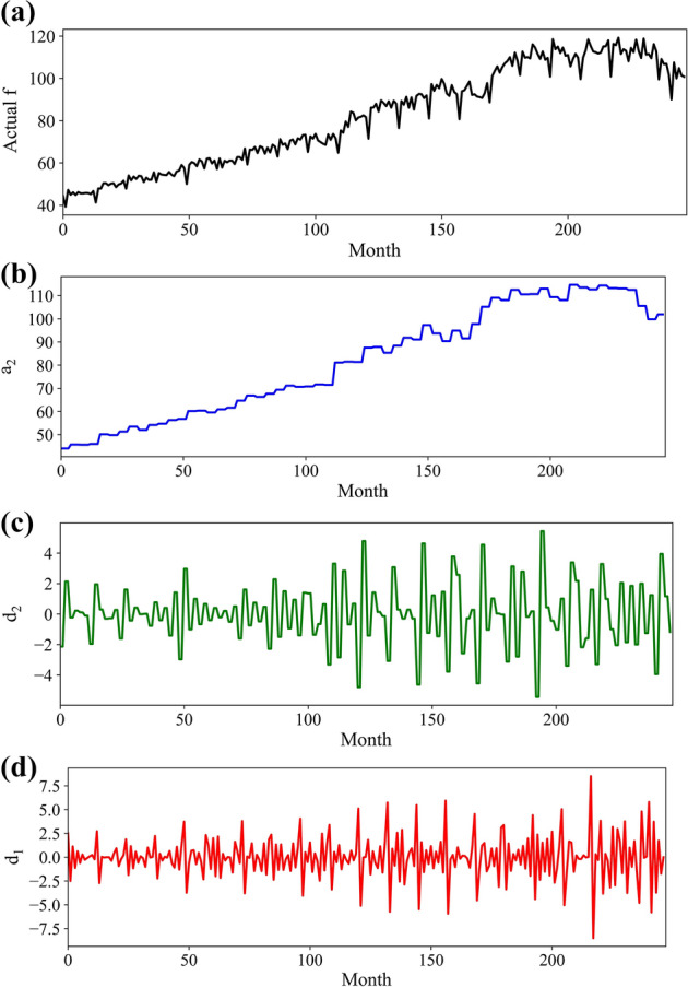
Port throughput employing DWT by denoising the 1D Level 2: a original data; b level 2 of the low-frequency component (a2); b and c Level 1 and 2 with high-frequency components (d1,d2)
Figure 6 shows the wavelet power spectra, illustrating the significant advantages of wavelet analysis over spectral analysis. The horizontal and vertical axes represent the time dimension and period, respectively. The color code indicates the range of the power spectra from blue (low power) to red (high power). It can be observed that the high power regions were distributed on periods of 27 to 45 across the entire vertical axis, beginning from 2002. The high-energy regions were widely and cyclically scattered, indicating a strong movement of cargo throughput over the entire developmental periods. This strong volatility resulted from the port development process, owing to the influences of many uncertain factors. The periodicity of the high-energy regions was due to seasonal demand, represented by the high-frequency component (d1 and d2) (González-Concepción et al. 2012).
Fig. 6.
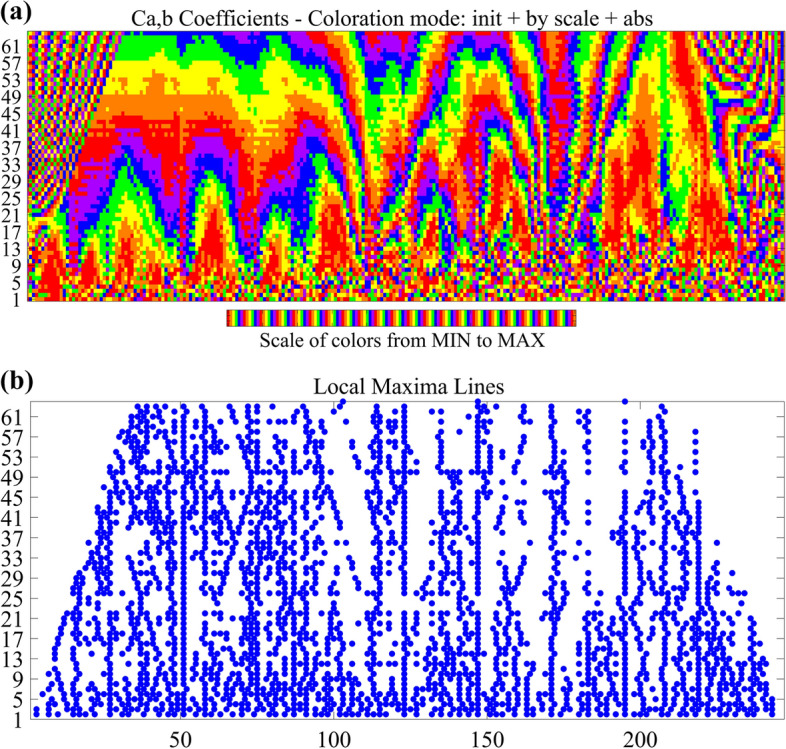
Power spectra of the cargo throughput via Haar wavelet: a signal analysis and b local maxima lines
Novel forecasting scheme employing the DWT–LSTM hybrid model
Conventional management mechanisms are generally designed to ensure stability, efficiency, and predictable performance. The cargo throughput of Busan Port is a complex dynamic system, open to environmental influences and susceptible to changing circumstances. These disruptions greatly impact short- and long-term development strategies. Therefore, a robust forecasting method, which decision-makers can rely on to improve operational efficiency, must be developed to guarantee the sustainability and profitability of the port. Machine learning algorithms can identify data patterns, learning from available data or observations. LSTM networks have recently demonstrated high effectiveness in time-series forecasting (Fischer and Krauss 2018; Punia et al. 2020). This machine learning scheme works well on linear and nonlinear time series behaviors (Punia et al. 2020). In this study, the cargo throughput data contain several patterns over volatile periods of international shipping, suggesting the LSTM strategy as a suitable alternative. In addition to the deep learning approach, wavelet transform can effectively convert cargo throughput datasets into low- and high-frequency series, and the decomposed series can be employed to forecast cargo throughput via the LSTM network (Chang et al. 2019). The extant experiments have demonstrated that the wavelet transform can efficiently support time-series forecasting (Schlüter and Deuschle 2010). In this study, a novel hybrid strategy, comprising DWT and the LSTM network, is proposed for cargo throughput forecasting.
LSTM model
LSTM networks represent a class of RNNs. RNN evaluates the relationship between the data entered in the past and future; it can excellently facilitate the analysis of continuous arrays of data. RNN is trained employing a backpropagation algorithm, after which it learns via the gradient descent method (Medsker and Jain 1999). Contrary to normal neural networks, RNN exhibits a recurrent learning structure and circulates input data according to the layers. This structure avails it with the memory of past information and updates it with the latest data. Figure 7 shows the memory cell of the LSTM structure.
Fig. 7.

Generic structures of the LSTM deep learning method
LSTM networks comprise input, several hidden, and output layers. The number of neurons in the input layer is equal to the number of explanatory variables (the feature space). The number of neurons in the output layer reflects the output space. The two neurons in this study determine whether a stock outperforms the cross-sectional median at t + 1 or not. The main characteristics of the LSTM networks are contained in the hidden layer(s) consisting of the so-called memory cells (Graves and Schmidhuber 2005). Each memory cell exhibits the following three gates that maintain and adjust its cell state, st: a forget gate (ft), an input gate (it), and an output gate (ot). At every time step, t, each of the three gates is presented with the input, xt (one element of the input sequence), and output, ht−1, of the memory cells at the previous time step, t–1. Thereafter, the gates act as filters, each fulfilling one of the purposes:
Forget gate defines the information to extract from the cell state.
Input gate specifies the information to add to the cell state.
Output gate specifies the information from the cell state that is utilized as output.
The formulas below are vectorized; they describe the update of the memory cells in the LSTM layer at every time step, t. The following notation is employed:
is the input vector at time step, t.
, and are weight matrices.
, and are bias vectors.
, and are the vectors of the activation values of the respective gates.
and are the vectors of the cell states and candidate values.
is a vector for the layer output.
During a forward pass, the cell states, st, and outputs, ht, of the layer at a time step, t, are calculated, as follows: in the first step, the LSTM layer determines the information that must be extracted from its previous cell states, st−1. Therefore, the activation values, ft, of the forget gates at t are computed employing the current input, xt; outputs, ht−1, of the memory cells at the previous (t − 1); and bias terms, bf, of the forget gates. The sigmoid function scales all the activation values in the range between 0 (completely forget) and 1 (completely remember):
| 6 |
In the second step, the LSTM layer determines the information that must be added to the network cell states (). This procedure comprises two operations. First, the candidate values (), which could be added to the cell states, are computed. Second, the activation values it of the input gates are calculated as follows:
| 7 |
| 8 |
In the third step, the new cell state () is calculated from the results of the two preceding steps, as follows:
| 9 |
where the symbol (◦) denotes the Hadamard (element-wise) product. In the final step, the outputs, ht, of the memory cells are derived, as follows:
| 10 |
| 11 |
When processing an input sequence, its features must be presented timestep by timestep to the LSTM network. Thus, the input at each timestep, t (in this study, one single standardized return), is processed by the network. The final output of the entire sequence is returned immediately after the last element of the sequence is processed.
DWT–LSTM hybrid model
To enhance the degree of the accuracy of predicting cargo throughput, a novel hybrid methodology is proposed, based on the DWT–LSTM model. The proposed approach can improve the existing forecasting method to cope with highly complex and chaotic trends. Figure 8 shows the overall process of the proposed methodology, which can be summarized in the following steps:
- Step (1).
Data decomposition: DWT decomposes the original cargo throughput into n components.
- Step (2).
Data characteristic analysis (DCA): all the decomposed components are thoroughly analyzed via the wavelet power spectra to determine the data characteristics.
- Step (3).
Individual predictions: based on DCA, one LSTM model was selected for the prediction of each component. Accordingly, the forecasting result of the corresponding component was obtained.
- Step (4).
Ensemble prediction: the predicted results of the components were combined with an aggregated cargo throughput.
- Step (5).
Performance evaluation: data analytics, as well as statistical analyses, were performed to assess the prediction results.
Fig. 8.

Hybrid scheme with a DWT–LSTM structure
The details of this scheme are also described in Algorithm 1, Appendix 3.
Empirical test results
Experimental setup and evaluation of the forecasting models
The future developments of a port can be predicted from trends, patterns, and current and historical throughput analysis. The time series employed in this study comprises data collected from cargo volumes of Busan Port. Cargo throughput is expressed as million tons (January 2001 to July 2021), and it is also available in the Korean PORT-MIS. Our monthly data consisted of 247 data points of import, export, and transshipment cargoes (Table 2). Typically, when constructing a model, the sample dataset is split into training and testing sets. Good data splitting will increase the robustness of the forecasting model and prevent overfitting or underfitting. In this study, the training and testing set utilized the same datasets for all forecasting methods. The training data were employed to teach an algorithm and generate forecasts for the data points, including 198 data points, within the testing set, covering the period from January 2001 to May 2017. The forecast evaluates the accuracy of the model by comparing the forecasted values with the observed values of the testing set (June 2017–July 2021); the more accurate the training data labels, the better the model will perform.
Table 2.
Dataset statistics for cargo throughput (cargo volume columns in million tons)
| Year | Total ships | Entry into port | Departure | |||
|---|---|---|---|---|---|---|
| Number of ships | Cargo volume | Number of ships | Cargo volume | Number of ships | Cargo volume | |
| Sum | 2,007,942 | 20,228.19 | 1,003,573 | 10,146.05 | 1,004,369 | 10,082.14 |
| Mean | 95,616.29 | 963.2473 | 47,789.19 | 483.1453 | 47,827.1 | 480.102 |
| SD | 12,869.1 | 284.3913 | 6466.564 | 143.9262 | 6402.67 | 140.4722 |
| Minimum | 46,704 | 541.141 | 23,186 | 270.3985 | 23,518 | 270.7425 |
| Maximum | 115,931 | 1361.337 | 57,979 | 684.9822 | 57,952 | 676.3552 |
The following four criteria are frequently employed to evaluate forecasting models: the mean squared error (MSE), mean absolute error (MAE), root mean squared error (RMSE), and root mean squared logarithmic error (RMSLE). MAE estimates the absolute difference between the actual and forecasted values. It can handle small actual values. The RMSE metric is obtained as the square root of MSE. This indicator is more sensitive to outliers than the mean absolute percentage error (MAPE). However, small actual values might produce misleadingly large MAPE values, whereas actual values close to zero can generate infinitely large MAPEs. RMSLE considers the relative error between the predicted and actual values, neglecting the scale of the data.
| 12 |
| 13 |
| 14 |
| 15 |
| 16 |
where and are the actual and forecasted values, respectively, and N is the sample size. A lower value indicates a more accurate model. To further compare performances, the Diebold–Mariano (DM) test was used to investigate the difference between the significance of forecasting performances (Diebold and Mariano 1995). Additionally, the Pesaran–Timmermann (PT) test was employed to evaluate the null hypotheses whereby the prediction is independently distributed for each forecasting method. The p-values of zero up to the fourth digit indicated that the null hypothesis can be rejected at any rational significance level (Pesaran and Timmermann 1995). Put differently, each machine learning method exhibits statistically significant predictive accuracy. In this study, the DM and PT tests were employed to evaluate the effectiveness of the proposed forecasting methods.
Forecasting results employing the hybrid algorithm.
Employing the hybrid prediction method, the original time series of cargo throughput was decomposed by the DWT technique. As discussed in Sect. 2.5, cargo throughput demonstrated highly complex dynamic behaviors. Figure 9 shows the managerial insights into the forecasting results that were obtained by our models. Figure 9a shows that the DWT–LSTM-based hybrid method produces better forecasting performance than single deep learning methods, such as RNN. The hybrid learning methods describe several details regarding the low-frequency (Fig. 9b) and high-frequency (Fig. 9c, d) components. Particularly, the test results indicated that the new hybrid approach produces the best performance: forecasting data accurately converged to their actual datasets. Although the RNN-based forecasting results showed that the model could not predict the dynamics of cargo throughput comprising high frequency components (d1 and d2), it availed underfitting prediction and larger prediction errors, a2, compared with the hybrid forecasting scheme. The average forecasting errors from each forecast are presented in Table 3. Based on all the performance indices, the hybrid forecasting strategy outperformed the existing benchmark methods.
Fig. 9.

Comparison of the models for forecasting the cargo throughput at Busan Port. a a2, b d1, and c d2
Table 3.
Performance comparison of forecasting algorithms (the smaller, the better)
| i j = | a1 | d2 | d1 | |||
|---|---|---|---|---|---|---|
| RNN | Proposed | RNN | Proposed | RNN | Proposed | |
| MAE | 11.9771 | 0.8079 | 5.4544 | 0.0713 | 12.4843 | 0.2848 |
| MSE | 2.6229 | 0.3075 | 1.9741 | 0.1508 | 2.6452 | 0.2534 |
| RMSE | 3.4607 | 0.8988 | 3.5333 | 0.2671 | 3.5333 | 0.5337 |
| MAPE | 0.0240 | 0.0029 | 0.0181 | 0.0696 | 1.1680 | 0.2062 |
| RMSLE | 0.0314 | 0.0085 | 0.0415 | 0.0175 | 0.0173 | 0.0073 |
Comparison of forecasting performance
To evaluate the effectiveness of our forecasting models, different tests were utilized, employing the hybrid model, plus other benchmark algorithms, including seasonal ARIMA (SARIMA), RNN, LSTM, and a gated recurrent unit (GRU). Many factors determine how much training data are required. More-complicated cases generally require more data than less-complex ones. Figure 10 shows the comparisons when the relative ratio of the training sample size is 80%. Notably, all the deep learning methods (RNN, LSTM, GRU, and the hybrid method) exhibited better forecasting patterns than the SARIMA model. The deep learning algorithms predicted the peak throughputs caused by disruptions. Moreover, the proposed algorithm delivered the best performance over the others, whereby the time series data converged completely to the actual data.
Fig. 10.

Comparison of the performances of forecasting models. a SARIMA, b RNN, c LSTM, d GRU, e DWT–LSTM (unit: million tons)
GRU and LSTM were the second- and third-best algorithms, respectively. The average relative forecasting errors are presented in Table 4 for model comparison. In this experiment, different ratios (60%, 70%, and 80%) of the training dataset to the sample size were employed. Notably, the bold font in the table indicates the best forecasting performance among the models. The test results showed that DWT–LSTM was the most accurate scheme. The proposed hybrid method outperformed the benchmark methods based on all five performance criteria. Particularly, when the relative ratio of the training sample size was set to 70% and 80%, the proposed hybrid algorithm delivered the best forecasts of cargo throughput. GRU, LSTM and RNN delivered the second-, third-, and fourth-best performances, respectively; SARIMA delivered the worst performance. However, when the training sample size was set to 60%, LSTM outperformed GRU, delivering the second-best performance. GRU was the third best, and the other ranking orders remained the same.
Table 4.
Forecasting model evaluation with different ratios of training sample sizes (the smaller, the better with bold indicating the top performer)
| Relative ratio | Performance indicator | MAE | MSE | RMSE | MAPE | RMSLE |
|---|---|---|---|---|---|---|
| 60% | SARIMA | 0.3523 | 1.0532 | 1.4577 | 1.3306 | 0.3747 |
| RNN | 0.1358 | 0.9376 | 1.5508 | 0.9334 | 0.7447 | |
| LSTM | 0.0631 | 0.1221 | 0.2907 | 0.2491 | 0.2731 | |
| GRU | 0.0785 | 0.2218 | 0.3158 | 0.2140 | 0.2907 | |
| DWT-LSTM | 0.0112 | 0.0168 | 0.0221 | 0.0286 | 0.0303 | |
| 70% | SARIMA | 0.2216 | 0.4100 | 0.4862 | 0.4224 | 0.5219 |
| RNN | 0.0839 | 0.1843 | 0.1052 | 0.1227 | 0.9535 | |
| LSTM | 0.0573 | 0.0942 | 0.1091 | 0.1328 | 0.1030 | |
| GRU | 0.04281 | 0.1066 | 0.1003 | 0.1207 | 0.1005 | |
| DWT-LSTM | 0.0066 | 0.0097 | 0.0113 | 0.0119 | 0.0101 | |
| 80% | SARIMA | 0.1144 | 0.5217 | 0.7875 | 0.6024 | 0.2247 |
| RNN | 0.0131 | 0.0694 | 0.1037 | 0.0352 | 0.0418 | |
| LSTM | 0.0232 | 0.2011 | 0.0934 | 0.0521 | 0.0442 | |
| GRU | 0.0291 | 0.3442 | 0.2297 | 0.1147 | 0.3751 | |
| DWT-LSTM | 0.0007 | 0.0011 | 0.0109 | 0.0114 | 0.0231 |
Moreover, for the empirical evaluation, statistical significance tests were conducted, employing the DM and PT tests. The monthly predictions of the training set at different ratios (60%, 70%, and 80%) are shown in Tables 5, 6, and 7, respectively. The test results show that the proposed method always outperforms the other benchmark methods, and the performance differences are statistically significant at the 95% confidence level. Panels A in Tables 5, 6, and 7 present the p-values of the DM test for the null hypothesis that the paired methods produce equal performances. The p-values present the confidence level that method i exhibits an inferior prediction accuracy to that of method j. All hypotheses were rejected at the 95% significance level, indicating that the proposed method is superior to all the benchmark ones regarding their forecasting performance. Panel B of each table presents the p-values of the PT test for the null hypothesis that the actual data and forecast values are independently distributed. It can be concluded with a high degree of certainty that the predictions from the forecasting models are independently distributed. All test results demonstrated that the proposed hybrid algorithm outperforms the other algorithms in forecasting cargo throughputs in a dynamic environment.
Table 5.
Statistical significance tests for port throughput when the relative ratio of the training sample size is 60% (panel A: DM test, panel B: PT test)
| i j = | A: DM test (p-value) | B: PT test (p-value) | |||||
|---|---|---|---|---|---|---|---|
| Proposed | SARIMA | RNN | LSTM | GRU | Method | Results | |
| Proposed | – | 0.0206 | 0.0003 | 0.0020 | 0.0001 | Proposed | 0.0000 |
| SARIMA | – | 0.0033 | 0.0006 | 0.0007 | SARIMA | 0.0000 | |
| RNN | – | 0.0010 | 0.0000 | RNN | 0.0000 | ||
| LSTM | – | 0.0000 | LSTM | 0.0000 | |||
| GRU | – | GRU | 0.0000 | ||||
Table 6.
Statistical significance tests for port throughput when the relative ratio of the training sample size is 70% (panel A: DM test, panel B: PT test)
| i j = | A: DM test (p-value) | B: PT test (p-value) | |||||
|---|---|---|---|---|---|---|---|
| Proposed | SARIMA | RNN | LSTM | GRU | Method | Results | |
| Proposed | – | 0.0011 | 0.0014 | 0.0000 | 0.0009 | Proposed | 0.0000 |
| SARIMA | – | 0.0033 | 0.0211 | 0.2077 | SARIMA | 0.0000 | |
| RNN | – | 0.0000 | 0.0000 | RNN | 0.0000 | ||
| LSTM | – | 0.0000 | LSTM | 0.0000 | |||
| GRU | – | GRU | 0.0000 | ||||
Table 7.
Statistical significance tests for port throughput when the relative ratio of the training sample size is 80% (panel A: DM test, panel B: PT test)
| i j = | A: DM test (p-value) | B: PT test (p-value) | |||||
|---|---|---|---|---|---|---|---|
| Proposed | SARIMA | RNN | LSTM | GRU | Method | Results | |
| Proposed | – | 0.0018 | 0.0000 | 0.0000 | 0.0009 | Proposed | 0.0000 |
| SARIMA | – | 0.0078 | 0.0137 | 0.3021 | SARIMA | 0.0000 | |
| RNN | – | 0.0010 | 0.0000 | RNN | 0.0000 | ||
| LSTM | – | 0.0000 | LSTM | 0.0000 | |||
| GRU | – | GRU | 0.0000 | ||||
Managerial insights and discussion
The collection and analysis of data can be expensive and time-consuming. The data analytics techniques presented here (LE, information entropy, HE, wavelet decomposition, statistical significance with DM, and the PT evaluation) are comprehensive and effective in analyzing nonlinear dynamical behaviors, as well as identifying business disruptions. Researchers have recently improved many business forecasting techniques, but have invested comparatively little in assessing prediction accuracies and efficiencies. However, biased forecasts can increase logistics costs (transportation, carrying, or warehousing costs), thus reducing profit margins.
Policymakers can employ different forecasting models to arrive at informed predictions. This study involves in-depth research on forecasting port throughput, showing at the same time our methods’ functionality and success. Forecasting algorithms, based on the hybrid deep learning method and four benchmark models, were presented to predict the cargo throughput of Busan Port. Holistically, the five metrics, as well as two statistical tests (DM and PT), demonstrated that the hybrid predictive approach outperforms the other benchmark algorithms with regard to all characteristics, ensuring higher forecasting accuracies and efficiencies. Our study was designed to confirm the superiority of deep learning models, such as GRU, LSTM, and RNN, over the traditional SARIMA models.
Moreover, for larger training sample sizes (70% and 80%), GRU outperformed LSTM, whereas LSTM was well suited for smaller training sample sizes. Indeed, for a training sample size of 60%, LSTM demonstrated a higher forecasting accuracy than GRU. It was also highlighted that the hybrid method outperforms LSTM and GRU in forecasting the time series. From the foregoing performance analyses, the following deep insights into cargo throughput can be mentioned: DWT represents a crucial pre-step for filtering the time series of cargo throughput data. The wavelet transform via deep learning outperformed the corresponding deep learning method in the absence of data decomposition. Particularly, the cargo throughput data exhibited highly complex and nonlinear behaviors in the presence of disruptions, including low- and high-frequency components. Although the traditional algorithms exhibited limitations in time series forecasting, the DWT methodology was efficient for decomposing the time-series data into different frequencies by filtering the data as a pre-treatment process. Thereafter, the prediction mechanisms based on deep learning models enhanced significantly the prediction accuracy and efficiency of each component to achieve the forecasting goals. The benefits of effective forecasting include improved business performances, gaining competitive advantage, offering rapid response to cyclical or seasonal change, identifying disruptions, and facilitating port strategic planning. Additionally, policymakers can exploit the novel forecasting model to keep their customers happy by delivering services and products while achieving strategic goals with profits in volatile markets.
Conclusions
We introduced the data analytics and forecasting algorithms for cargo throughput forecasts at the port of Busan. First, time-series data analysis was conducted, employing nonlinear analysis tools. Specifically, dynamic analysis tools for exploring the underlying mechanisms of maritime logistics under the impact of market volatility included LE, information entropy, HE, and wavelet decomposition. According to the system behavior revealed by the nonlinear paradigms, the cargo throughput dynamics of the port exhibited highly complex and chaotic behaviors against uncertainties and external disruptions. These drastic throughput changes were mainly caused by market disruptions, such as seasonal demand, the 2009 global financial crisis, and the ongoing COVID-19 pandemic. The results can help port managers understand the nature of complexities and the dynamics of port operations.
Next, a robust forecasting method was proposed, employing the wavelet transform and deep learning methods. The proposed approach was compared with other benchmark methods against supply chain disruptions. Three different ratios (60%, 70%, and 80%) were employed for the training set samples. For a forecasting benchmark, different common methods, including SARIMA, RNN, LSTM, and GRU, were employed in the tests. Further, five performance metrics, comprising MSE, MAE, MAPE, RMSE, and RMSLE, were employed to evaluate the algorithms. The DM and PT statistical significance tests were used to confirm the key empirical findings. The evaluation results indicated that the proposed method outperforms all other benchmarks that are widely employed in the data science community. Our hybrid strategy combined the DWT and LSTM methods (DWT–LSTM), enhancing the degree of prediction accuracy and efficiency by simply denoising cargo throughput data. This method was optimized by combining the advantages of DWT and LSTM to obtain the target outcomes. Another finding is that predictions employing GRU are more accurate than those employing LSTM in cases involving large training datasets. On the other hand, LSTM was superior to GRU for smaller training datasets.
To summarize, our study contributes to the theories and practices of data analytics and business forecasting. Our first contribution is the proposal of powerful tools for investigating nonlinear datasets and complex dynamics. This can help policymakers gain greater insight into the dynamic behavior of seaport operations as well as explore disruption mechanisms. Second, our study has presented a robust and flexible forecasting method, which can be employed to predict complex maritime logistics patterns for achieving business goals. Therefore, these findings, reached by employing the proposed methods, can help decision-makers to prepare better for future port operations against maritime disruptions.
Acknowledgements
This research was supported by Korea Institute of Marine Science & Technology Promotion (KIMST), funded by the Ministry of Oceans and Fisheries, Korea (20220573). The authors are grateful to helpful MEL reviews.
Appendix 1
For a time series length, the m-dimensional vector at the time i can be given by
| 17 |
where denotes data in new time series, m is the embedding dimension and is the time delay. The has a permutation , when satisfies the following condition:
| 18 |
where and . It can be obtained from Eq. (18) that an m-tuple vector has m! possible distributions. Moreover, the calculation of frequency of distribution is given as
| 19 |
where represents the number of , and it is consistent with the type . Then, the PE with m-dimensions can be described as
| 20 |
It is noted that when , is reaching the maximum value . The PE measure can be normalized through as
| 21 |
Appendix 2
The Hurst exponent analysis steps are given as follows:
Determine the mean
| 22 |
Evaluate the adjusted mean series Y,
| 23 |
Calculate the cumulative deviation Z,
| 24 |
Determine the range series R,
| 25 |
Compute the standard deviation S,
| 26 |
where u is the mean value from X1 to Xt. Next, the rescaled range can be given as
| 27 |
Note that (R/S)t is the averaged over the regions [X1, Xt], [Xt+1, X2t] until [X(m−1)t+1, Xmt], where m = ⌊N/t⌋. To use all data for calculations, a value of t is chosen such that it is divisible by N. The relationship between (R/S)t and the Hurst exponent (H) is calculated by
| 28 |
where cα is a constant. To estimate the Hurst exponent, (R/S) versus t in log–log axes can be plotted. The slope of the curve is estimated using the ordinary least squares (OLS) scheme.
Appendix 3
| Algorithm 1: Forecasting based on hybrid algorithm | |||
| Input: Data input , training data length Ly, A LSTM model with P layers, weight W, training epoch n | dataset to be used | ||
| Output: Predicted throughput and error | |||
| 1 | Decompose into a2 + d2 + d1 | DWT technique | |
| 2 | ; | ||
| 3 | Set | training data | |
| for ( j = 1 to 3) | |||
| 4 | while do | ||
| 5 | |||
| 6 | LSTM input | ||
| 7 | input gate | ||
| 8 | forget gate | ||
| 9 | cell | ||
| 10 | output gate | ||
| 11 | LSTM output | ||
| 12 | end | ||
| 13 | end | ||
| 14 | Prediction results: | ||
| 15 | average pooling | ||
| 16 | Compute | ||
| 17 | Find | index of highest probability | |
| 18 | predicted output of each component | ||
| 19 | invert DWT | ||
| 20 | predicted error | ||
| 21 | End procedure | ||
Footnotes
Publisher's Note
Springer Nature remains neutral with regard to jurisdictional claims in published maps and institutional affiliations.
References
- Bandt C, Pompe B. Permutation entropy: A natural complexity measure for time series. Physical Review Letters. 2002;88(17):174102. doi: 10.1103/PhysRevLett.88.174102. [DOI] [PubMed] [Google Scholar]
- Barzegar R, Aalami MT, Adamowski J. Short-term water quality variable prediction using a hybrid CNN–LSTM deep learning model. Stochastic Environmental Research and Risk Assessment. 2020;34(2):415–433. doi: 10.1007/s00477-020-01776-2. [DOI] [Google Scholar]
- Chang Z, Zhang Y, Chen W. Electricity price prediction based on hybrid model of Adam optimized LSTM neural network and wavelet transform. Energy. 2019;187:115804. doi: 10.1016/j.energy.2019.07.134. [DOI] [Google Scholar]
- Clément A, Laurens S. An alternative to the Lyapunov exponent as a damage sensitive feature. Smart Materials and Structures. 2011;20(2):025017. doi: 10.1088/0964-1726/20/2/025017. [DOI] [Google Scholar]
- Corazza M, Malliaris ATG. Multi-fractality in foreign currency markets. Multinational Finance Journal. 2002;6(2):65–98. doi: 10.17578/6-2-1. [DOI] [Google Scholar]
- Cuong TN, Kim HS, Xu X, You SS. Container throughput analysis and seaport operations management using nonlinear control synthesis. Applied Mathematical Modelling. 2021;100:320–341. doi: 10.1016/j.apm.2021.07.039. [DOI] [Google Scholar]
- Cullinane K, Haralambides H. Global trends in maritime and port economics: The COVID-19 pandemic and beyond. Maritime Economics & Logistics. 2021;23(3):369–380. doi: 10.1057/s41278-021-00196-5. [DOI] [Google Scholar]
- Diebold FX, Mariano RS. Comparing predictive accuracy. Journal of Business and Economic Statistics. 1995;13:253–263. [Google Scholar]
- Dirzka C, Acciaro M. Global shipping network dynamics during the COVID-19 pandemic's initial phases. Journal of Transport Geography. 2021;99:103265. doi: 10.1016/j.jtrangeo.2021.103265. [DOI] [PMC free article] [PubMed] [Google Scholar]
- Du P, Wang J, Yang W, Niu T. Container throughput forecasting using a novel hybrid learning method with error correction strategy. Knowledge-Based Systems. 2019;182:104853. doi: 10.1016/j.knosys.2019.07.024. [DOI] [Google Scholar]
- Ferreira KJ, Lee BHA, Simchi-Levi D. Analytics for an online retailer: Demand forecasting and price optimization. Manufacturing & Service Operations Management. 2016;18(1):69–88. doi: 10.1287/msom.2015.0561. [DOI] [Google Scholar]
- Feder, J. 1988. Fractals. New York: Plenum Press.
- Fischer T, Krauss C. Deep learning with long short-term memory networks for financial market predictions. European Journal of Operational Research. 2018;270(2):654–669. doi: 10.1016/j.ejor.2017.11.054. [DOI] [Google Scholar]
- González-Concepción C, Gil-Fariña MC, Pestano-Gabino C. Using wavelets to understand the relationship between mortgages and Gross Domestic Product in Spain. Journal of Applied Mathematics. 2012 doi: 10.1155/2012/917247. [DOI] [Google Scholar]
- Gou X, Lam JSL. Risk analysis of marine cargoes and major port disruptions. Maritime Economics & Logistics. 2019;21(4):497–523. doi: 10.1057/s41278-018-0110-3. [DOI] [Google Scholar]
- Gosasang V, Chandraprakaikul W, Kiattisin S. A comparison of traditional and neural networks forecasting techniques for container throughput at Bangkok port. The Asian Journal of Shipping and Logistics. 2011;27(3):463–482. doi: 10.1016/S2092-5212(11)80022-2. [DOI] [Google Scholar]
- Graves A, Schmidhuber J. Framewise phoneme classification with bidirectional LSTM and other neural network architectures. Neural Networks. 2005;18(5–6):602–610. doi: 10.1016/j.neunet.2005.06.042. [DOI] [PubMed] [Google Scholar]
- Hochreiter, S., and J. Schmidhuber. 1997. Long short-term memory. Neural Computation 9 (8): 1735–1780. [DOI] [PubMed]
- Hurst, H.E. 1951. Long-term storage capacity of reservoirs. Transactions of the American Society of Civil Engineers 116 (1): 770–799.
- Hwarng HB, Xie N. Understanding supply chain dynamics: A chaos perspective. European Journal of Operational Research. 2008;184(3):1163–1178. doi: 10.1016/j.ejor.2006.12.014. [DOI] [Google Scholar]
- Islam S, Amin SH. Prediction of probable backorder scenarios in the supply chain using Distributed Random Forest and Gradient Boosting Machine learning techniques. Journal of Big Data. 2020;7(1):1–22. doi: 10.1186/s40537-020-00345-2. [DOI] [Google Scholar]
- Jahanshahi H, Yousefpour A, Wei Z, Alcaraz R, Bekiros S. A financial hyperchaotic system with coexisting attractors: Dynamic investigation, entropy analysis, control and synchronization. Chaos, Solitons & Fractals. 2019;126:66–77. doi: 10.1016/j.chaos.2019.05.023. [DOI] [Google Scholar]
- Johannesen NJ, Kolhe M, Goodwin M. Relative evaluation of regression tools for urban area electrical energy demand forecasting. Journal of Cleaner Production. 2019;218:555–564. doi: 10.1016/j.jclepro.2019.01.108. [DOI] [Google Scholar]
- Justice V, Bhaskar P, Pateman H, Cain P, Cahoon S. US container port resilience in a complex and dynamic world. Maritime Policy & Management. 2016;43(2):179–191. doi: 10.1080/03088839.2015.1133937. [DOI] [Google Scholar]
- Lam JSL, Notteboom T. The greening of ports: A comparison of port management tools used by leading ports in Asia and Europe. Transport Reviews. 2014;34(2):169–189. doi: 10.1080/01441647.2014.891162. [DOI] [Google Scholar]
- Lee Y, Song H, Jeong S. Prioritizing environmental justice in the port hinterland policy: Case of Busan New Port. Research in Transportation Business & Management. 2021;41:100672. doi: 10.1016/j.rtbm.2021.100672. [DOI] [Google Scholar]
- Liaw, S.S., and F.Y. Chiu. 2009. Fractal dimensions of time sequences. Physica A 338: 3100–3106.
- Lin W, Wu Z, Lin L, Wen A, Li J. An ensemble random forest algorithm for insurance big data analysis. IEEE Access. 2017;5:16568–16575. doi: 10.1109/ACCESS.2017.2738069. [DOI] [Google Scholar]
- Liu Yan, Chen Yi-Mei. Application of grey system model in throughput forecasting of inland river port. Port & Waterway Engineering. 2006;4:31. [Google Scholar]
- Medsker L, Jain LC, editors. Recurrent neural networks: Design and applications. Boca Raton: CRC Press; 1999. [Google Scholar]
- Memarzadeh G, Keynia F. A new short-term wind speed forecasting method based on fine-tuned LSTM neural network and optimal input sets. Energy Conversion and Management. 2020;213:112824. doi: 10.1016/j.enconman.2020.112824. [DOI] [Google Scholar]
- Morris SA, Pratt D. Analysis of the Lotka-Volterra competition equations as a technological substitution model. Technological Forecasting and Social Change. 2003;70(2):103–133. doi: 10.1016/S0040-1625(01)00185-8. [DOI] [Google Scholar]
- Notteboom T. The adaptive capacity of container ports in an era of mega vessels: The case of upstream seaports Antwerp and Hamburg. Journal of Transport Geography. 2016;54:295–309. doi: 10.1016/j.jtrangeo.2016.06.002. [DOI] [Google Scholar]
- Pesaran MH, Timmermann A. Predictability of stock returns: Robustness and economic significance. The Journal of Finance. 1995;50(4):1201–1228. doi: 10.1111/j.1540-6261.1995.tb04055.x. [DOI] [Google Scholar]
- Punia S, Nikolopoulos K, Singh SP, Madaan JK, Litsiou K. Deep learning with long short-term memory networks and random forests for demand forecasting in multi-channel retail. International Journal of Production Research. 2020;58(16):4964–4979. doi: 10.1080/00207543.2020.1735666. [DOI] [Google Scholar]
- Rajaee, T., V. Nourani, M. Zounemat-Kermani, and O. Kisi. 2011. River suspended sediment load prediction: application of ANN and wavelet conjunction model. Journal of Hydrologic Engineering 16 (8): 613–627.
- Saini S, Roy D, de Koster R. A stochastic model for the throughput analysis of passing dual yard cranes. Computers & Operations Research. 2017;87:40–51. doi: 10.1016/j.cor.2017.05.012. [DOI] [Google Scholar]
- Schlüter, S., and C. Deuschle. 2010. Using wavelets for time series forecasting: Does it pay off? (No. 04/2010). IWQW Discussion Papers.
- Schulze PM, Prinz A. Forecasting container transhipment in Germany. Applied Economics. 2009;41(22):2809–2815. doi: 10.1080/00036840802260932. [DOI] [Google Scholar]
- Shankar S, Punia S, Ilavarasan PV. Deep learning-based container throughput forecasting: A triple bottom line approach. Industrial Management & Data Systems. 2021 doi: 10.1108/IMDS-12-2020-0704. [DOI] [Google Scholar]
- Sipper, M., and J.H. Moore 2021. Conservation machine learning: a case study of random forests. Scientific Reports 11 (1): 3629. [DOI] [PMC free article] [PubMed]
- Slotine JJE, Li W. Applied nonlinear control. Englewood Cliffs, NJ: Prentice Hall; 1991. [Google Scholar]
- Sprott JC. Chaos data Analyzer (Professional Version) Raleigh, NC: Physics Academic Software; 1995. [Google Scholar]
- Tetteh, E.A., H.L. Yang, and F. Gomina Mama. 2016. Container ports throughput analysis: a comparative evaluation of China and five west African Countries' seaports efficiencies. In International Journal of Engineering Research in Africa (Vol. 22, pp. 162–173). Trans Tech Publications Ltd.
- Twrdy E, Batista M. Modeling of container throughput in Northern Adriatic ports over the period 1990–2013. Journal of Transport Geography. 2016;52:131–142. doi: 10.1016/j.jtrangeo.2016.03.005. [DOI] [Google Scholar]
- Tzouras S, Anagnostopoulos C, McCoy E. Financial time series modeling using the Hurst exponent. Physica A: Statistical Mechanics and Its Applications. 2015;425:50–68. doi: 10.1016/j.physa.2015.01.031. [DOI] [Google Scholar]
- Wolf A, Swift JB, Swinney HL, Vastano JA. Determining Lyapunov exponents from a time series. Physica D: Nonlinear Phenomena. 1985;16(3):285–317. doi: 10.1016/0167-2789(85)90011-9. [DOI] [Google Scholar]
- Xie G, Zhang N, Wang S. Data characteristic analysis and model selection for container throughput forecasting within a decomposition-ensemble methodology. Transportation Research Part E: Logistics and Transportation Review. 2017;108:160–178. doi: 10.1016/j.tre.2017.08.015. [DOI] [Google Scholar]
- Yang CH, Chang PY. Forecasting the demand for container throughput using a mixed-precision neural architecture based on CNN–LSTM. Mathematics. 2020;8(10):1784. doi: 10.3390/math8101784. [DOI] [Google Scholar]
- Yao CZ, Lin JN, Liu XF, Zheng XZ. Dynamic features analysis for the large-scale logistics system warehouse-out operation. Physica A: Statistical Mechanics and Its Applications. 2014;415:31–42. doi: 10.1016/j.physa.2014.07.077. [DOI] [Google Scholar]
- Ye Y, Zhang Y, Wang Q, Wang Z, Teng Z, Zhang H. Fault diagnosis of high-speed train suspension systems using multiscale permutation entropy and linear local tangent space alignment. Mechanical Systems and Signal Processing. 2020;138:106565. doi: 10.1016/j.ymssp.2019.106565. [DOI] [Google Scholar]
- Zhang, W., and J.S.L. Lam. 2017. An empirical analysis of maritime cluster evolution from the port development perspective – Cases of London and Hong Kong. Transportation Research Part A: Policy and Practice 105: 219–232.
- Zhang N, Shen SL, Zhou A, Jin YF. Application of LSTM approach for modelling stress–strain behaviour of soil. Applied Soft Computing. 2021;100:106959. doi: 10.1016/j.asoc.2020.106959. [DOI] [Google Scholar]
- Zuo Y, Fu X, Liu Z, Huang D. Short-term forecasts on individual accessibility in bus system based on neural network model. Journal of Transport Geography. 2021;93:103075. doi: 10.1016/j.jtrangeo.2021.103075. [DOI] [Google Scholar]