Characterization and Stratification of Prostate Lesions Based on Comprehensive Multiparametric MR Imaging Using Detailed Whole Mount Histopathology as a Reference Standard

Abstract

The purpose of this study was to characterize prostate cancers (PCa) based on multiparametric MR (mpMR) measures derived from MRI, diffusion, spectroscopy, and dynamic contrast-enhanced (DCE) MRI and to validate mpMRI in detecting PCa and predicting PCa aggressiveness by correlating mpMRI findings with whole-mount histopathology. Seventy-eight men with untreated PCa received 3T-mpMR scans prior to radical prostatectomy. Cancerous regions were outlined, graded, and cancer amount estimated on whole-mount histology. Regions of interest were manually drawn on T2-weighted images based on histopathology. Logistic regression (LR) was used to identify optimal combinations of parameters to separate 1) benign from malignant tissues, 2) Gleason Score (GS) ≤3+3 disease from ≥GS3+4, and 3) ≤GS3+4 from ≥GS4+3 cancers for peripheral zone (PZ) and transition zone (TZ). Performance of the models was assessed using repeated four-fold cross-validation. Additionally, the performance of the logistic regression models created under the assumption that one or more modality has not been acquired was evaluated. LR models yielded area under the curve (AUC) of 1.0 and 0.99 when separating benign from malignant tissues in the PZ and the TZ, respectively. Within PZ, combining choline, maximal enhancement slope, ADC, and citrate measures for separating ≤GS3+3 from ≥GS3+4 PCa yielded AUC=0.84. Combining creatine, choline, and washout slope yielded AUC=0.81 for discriminating ≤GS3+4 from ≥GS4+3 disease. Within TZ, combining washout slope, ADC, and creatine yielded AUC=0.93 for discriminating ≤GS3+3 and ≥GS3+4 cancers. When separating ≤GS3+4 from ≥GS4+3 PCa, combining choline and washout slope yielded AUC=0.92. MpMRI provides excellent separation between benign tissues and PCa, and across PCa tissues of different aggressiveness. The final models prominently featured spectroscopy and DCE-derived metrics underlining their value within a comprehensive mpMRI exam.

1. Introduction

Approximately one in seven men in the United States will receive a prostate cancer (PCa) diagnosis during his lifetime.¹ Given the often indolent nature of the prostate tumors and potentially adverse consequences of the available treatments, accurate disease risk stratification is essential for identifying patient-specific cancer management strategies.² Currently, prostate-specific antigen and digital rectal exam are the main diagnostic tools used in prostate cancer screening.³ Suspicious findings on these noninvasive modalities are typically followed by a transrectal ultrasound-guided biopsy with the assigned Gleason grade of any detected malignancy being one of the most powerful predictors of patient outcome.⁴

Despite this, accuracy of Gleason score based on biopsy findings frequently suffers from inadequate tumor sampling with biopsy Gleason score underestimating actual Gleason score in up to 45% of radical prostatectomy cases.⁵ More than 30% of cancers are missed on transrectal ultrasound-guided prostate biopsies altogether.⁵ Furthermore, prostate biopsy is not a benign procedure, and can be associated with discomfort, pain, hematuria, rectal bleeding, risk of severe infection, and death.⁶ Multiparametric magnetic resonance imaging is a noninvasive technique that can be used for detection and localization of prostate cancer.

The utility of diffusion weighted imaging (DWI), T2-weighted imaging, magnetic resonance spectroscopic (MRS), and Dynamic contrast-enhanced (DCE) sequences in detecting and localizing prostate cancer is well documented in literature.^7,8 The next pertinent question is whether mpMRI can be used to accurately determine the aggressiveness of the disease. Several studies have examined various imaging parameters as potential biomarkers for Gleason score, and have yielded mixed results for Gleason score correlations with T2-weighted imaging,⁹ ADC,^10–13 MRS^14,15 and DCE MRI.^11,16,17 The purpose of this study was to use a logistic regression approach to improve the characterization of prostate cancers based on multiparametric MR measures derived from MRI, diffusion, spectroscopy, and dynamic contrast-enhanced MRI and to validate mpMRI in detecting PCa and in predicting PCa aggressiveness by correlating mpMRI findings with whole-mount histopathology generated from radical prostatectomy specimens.

2. Materials and Methods

2.1. Patients

This study was approved by the Committee on Human Research at this institution and was compliant with the Health Insurance Portability and Accountability Act. Seventy-eight patients were studied. Two sets of patients were pooled for this study: 1) patients scheduled for surgery, recruited during a urological oncology clinic to receive mpMRI prior to surgery identified prospectively and 2) patients who received mpMRI and then pursued surgical treatment post imaging identified retrospectively. Written, informed consent was obtained from all subjects. Patients who underwent any treatment for their prostate cancer prior to surgery, or whose surgery was more than a year after their MRI were excluded from the study. No MRI exam was performed less than 6 weeks after prostate biopsy.

2.2. MR Imaging

All patients were imaged with an expandable balloon endorectal coil (MedRad, Bayer HealthCare LLC, Whippany, NJ) combined with an external phased array coil on a 3T MR scanner (GE Healthcare, Waukesha, WI, USA). A perfluorocarbon fluid (Galden; Solvay Plastics, West Deptford, NJ, USA) was used to inflate the balloon coil. Fast spin echo (FSE) T2-weighted images were acquired in an oblique axial plane with FOV = 18cm, slice thickness = 3mm, matrix = 512×512, and TR/TE = 6000/96ms. Diffusion weighted imaging (DWI) was acquired using a 2D single-shot spin echo sequence TR/TE=4000/78-90ms, pixel bandwidth = 1952 (conventional acquisition), pixel bandwidth = 1305 (reduced-field-of-view acquisition¹⁸), b=0 and 600 s/mm², slice thickness=3mm. MRSI data was acquired using a 3D flyback, echo planar PRESS CSI acquisition, with a 16×12×10 matrix, acquired at 5.4 mm resolution, zero-filled to 5.4×2.7×2.7mm³, 0.04cc voxels, TR/TE=2000/85ms,¹⁹ MRSI data was not available in 4/78 subjects (2 had technical errors and 2 were not acquired). DCE MRI was performed using a 3D fast SPGR sequence with TR/TE = 3.5/0.9ms, flip angle = 5°, slice thickness = 3mm slices, and a single-dose of gadopentetate dimeglumine (Gd-DTPA) (Magnevist; Bayer, Whippany, NJ) over ~5 minutes. The acquisition parameters are outlined in Appendix A. T2-weighted images and MRSI were corrected for the inhomogeneous reception profile associated with the combined endorectal coil and the external phased array.²⁰ Apparent diffusion coefficient (ADC) maps were created using an in-house software, from the combined DWI (b=600 s/mm²) and T2-weighted reference images (b=0 s/mm²) using Eq. (1), where b is the b-value used for the diffusion-weighted acquisition reflecting the gradient strength and duration, S_gm is the geometric mean of the signal intensity over the six gradient directions, and S₀ is the signal intensity of the T2-weighted image acquired without diffusion gradients. The calculation was done on a voxel-by-voxel basis.

$$\text{ADC}=-\frac{1}{\text{b}}\ln (\frac{{\text{S}}_{\text{gm}}}{{\text{S}}_0})$$ [1]

Choline, creatine, and citrate levels were quantified by measuring the height of the peaks. Additionally, [Choline+Creatine]/Citrate ([Cho+Cre]/Cit), as well as Choline/Citrate (Cho/Cit) and Choline/Creatine (Cho/Cre) ratios were computed. DCE MRI maps were created based on the semi-quantitative tissue enhancement parameters of peak enhancement, maximal enhancement slope, and washout rate.²¹ Additionally, pharmacokinetic modeling was applied to the data using the assumption that the fractional plasma volume (v_p) was 0.01.²² The concentration of Gd-DTPA in the plasma was modeled as a biexponential Eq. (2)

$${\text{C}}_{\text{p}}=\text{AmpD}({\text{a}}_1{\text{e}}^{-{\text{m}}_1\text{t}}+{\text{a}}_2{\text{e}}^{-{\text{m}}_2\text{t}})$$ [2]

where Amp=4, D = 0.1mmol/Kg of Gd-DTPA, a₁ = 3.99 kg/L, m₁ = 0.144 1/min, a₂ = 4.78 kg/L, m₂ = 0.011 1/min. The Amp was introduced to account for an offset between our experimental measures and this population average and was determined by minimizing the root-mean-square error (RMSE) of the fits.

A novel pharmacokinetic Luminal Water (LW) model was used.²³ In the LW model, a luminal water fractional volume parameter (v_l) is introduced to the extended Tofts Kermode model.²² The model is designed based on the assumption that Gd-DTPA does not reach intact prostatic ductal lumen, preventing the water in the lumen from interacting with gadolinium molecules. The non-linear LW model was fitted to data using non-linear least squares estimation with the “optim” function in R (R Foundation for Statistical Computing, Vienna, Austria).²⁴ The quantitative DCE parameters of the transfer constant (K^trans), the fractional extravascular, extracellular volume (v_ees), the rate constant (k_ep) and v_l were computed. As the LW model is an extension of the Tofts Kermode model, only the LW model was used to avoid redundancy in the parameters and to provide the additional parameter of v_l.

2.3. Histopathology

Post prostatectomy, all prostate specimens were fixed using injected neutral-buffered formalin for at least 24 hours and then serially cross-sectioned from apex to base at 3mm intervals using a manual meat slicer (Hobart, Troy, OH, USA). All slices were then embedded in paraffin as whole-mount sections, cut at 4 micron thickness, stained with hematoxylin and eosin, and examined under light microscopy by the study pathologist with regions of interest marked. The slides were then digitally scanned for comparison to the MR images.

2.4. Identifying Regions of Interest

During histological review, cancerous regions on each slide were outlined and graded by the study pathologist using the Gleason system; the amount of cancer in each region was estimated, along with the various fractions of each Gleason grade in each cancer region. Benign tissue regions of cystic atrophy (dilated cystic glands) and normal prostate glandular tissue were also identified and outlined. Next, regions of interest were manually drawn freeform on T2-weighted images based on the digitized histopathology slides using anatomical cues, following a consensus of two readers, keeping within homogeneous regions.

Only regions of interest (ROIs) with areas larger than 0.05cc were included in the analysis. ROIs were grouped based on region within the prostate (peripheral zone versus transition zone) and tissue of interest – cystic atrophy/normal tissue or Gleason Grade groups. For each patient, average imaging parameters were computed across the ROIs in question, weighted by the ROI area, resulting in one measure per patient for each tissue grouping.

2.5. Statistical Analysis

Statistical analysis was carried out using the JMP software (JMP, Version 10, SAS Institute Inc., Cary, NC). A p-value of 0.05 or less was used to define statistical significance. Descriptive statistics were listed as mean ± standard deviation when normally distributed and as median (first quartile (Q1), third quartile (Q3)) when not normally distributed. Non-parametric Wilcoxon signed-rank paired tests were used to compare all the imaging parameters of interest across tissue types. For the four subjects with missing MRSI data, mean MRSI values over ROIs within the group of interest were substituted for the missing MRSI values in order to include these four patients in the analysis. A stepwise logistic regression analysis was performed for all imaging modalities and combinations of imaging parameters. A mixed stepwise logistic regression with a threshold p-value of 0.15 was used to identify the imaging parameters to be included or excluded in the combined model. While multiple parameters from one modality, i.e. DCE MRI or MRSI, have some inherent dependencies, due to being from the same acquisition, they also can contain unique information. For instance, both DCE MRI and MRSI contain an additional dimension of data (time with DCE MRI and frequency with MRSI). Thus, multiple parameters from individual modalities were tested for inclusion in the combined models. The area under the ROC (receiver operating characteristic) curve (AUC) was computed and its performance was evaluated in distinguishing 1) benign tissues from malignant, 2) ≤GS3+3 disease from ≥GS3+4 PCa, and 3) ≤GS3+4 disease from ≥GS4+3 PCa. Sensitivity and specificity values were also reported. Optimal sensitivity and specificity pairs were chosen off of the ROC curve with the assumption that false negatives and false positives come at similar costs. Separate analyses were carried out for the transition zone and the peripheral zone tissues. To assess performance of each model, repeated k-fold cross-validation with 10 iterations and k=4 was performed.

Additionally, the performances of the models created under the assumption that one or more modality has not been acquired were evaluated. The AUC ROC values were computed for distinguishing 1) benign tissues from malignant, 2) ≤GS3+3 disease from ≥GS3+4 PCa, and 3) ≤GS3+4 disease from ≥GS4+3 PCa for seven different acquisition scenarios. The following combinations of modalities were considered: 1) T2-weighted imaging and DWI, 2) T2-weighted imaging and DCE, 3) T2-weighted imaging and MRSI, 4) T2-weighted imaging, DWI, and DCE, 5) T2-weighted imaging, DCE, and MRSI, 6) T2-weighted imaging, DWI, and MRSI, and finally 7) when all modalities were acquired.

3. Results

No adverse events due to mpMRI scans performed in the course of this study were reported. The patients’ mean age was 63.7±6.3 years, the median pre-surgical PSA was 6.2 ng/ml (Q1=4.3 ng/ml, Q3=8.35 ng/ml), the median prostatectomy Gleason score was 7 (Q1=6, Q3=8), ranging from GS 6 to GS 10. For this study, the median time interval between MRI scan and prostatectomy was 40 days (Q1=14 days, Q3=83.8 days), ranging from 2 to 201 days.

The distribution of Gleason scores across patients, the ROI numbers, and lesion-based ROI sizes used in the analyses are summarized in Table 1. In the peripheral zone 291 cancer ROIs were drawn for 65 patients, while in the transition zone 125 cancer ROIs were drawn for 24 patients. Sixteen cases had both peripheral zone and transition zone lesions. The median size of these averaged, lesion-based ROIs in the peripheral zone was 0.30cc (Q1=0.13cc, Q3=0.52cc), ranging from 0.05cc to 8.28cc, while in the transition zone the median lesion-based ROI size was 0.28cc (Q1=0.16cc, Q2=0.66cc), ranging from 0.05cc to 2.05cc.

Table 1:

Patient, region of interest (ROI) counts, and lesion based ROI sizes for healthy and cancerous tissues.

Prostate Region	Tissue Type	Number of Patients	Number of ROIs	Median (Q1, Q3) Lesion-based ROI size (cc)
Peripheral Zone	Benign	67	218	0.31 (0.16, 0.59)
	3+2	1	1	0.08 (0.08, 0.08)
	3+3	31	84	0.30 (0.07, 0.30)
	3+4	27	83	0.35 (0.13, 0.58)
	4+3	20	47	0.23 (0.15, 0.62)
	4+4	11	23	0.17 (0.13, 0.30)
	4+5	5	24	1.03 (0.43, 3.28)
	5+3	2	10	1.06 (0.71, 1.41)
	5+4	3	9	0.32 (0.30, 0.57)
	5+5	2	10	4.29 (2.30, 6.28)
Transition Zone	Benign	42	126	0.28 (0.12, 0.59)
	3+2	4	11	0.33 (0.26, 0.41)
	3+3	15	45	0.24 (0.15, 0.38)
	3+4	11	37	0.39 (0.25, 0.80)
	4+3	9	25	0.18 (0.15, 0.64)
	4+4	2	5	0.65 (0.37, 0.93)
	3+5	1	2	0.30 (0.30, 0.30)

Benign regions include cystic atrophy and normal peripheral zone tissues.

Not normally distributed data reported as median (first quartile (Q1), third quartile (Q3)).

An example of mpMR images obtained as part of the study and corresponding histopathological slides are illustrated in Figure 1 for a peripheral zone cancer and in Figure 2 showing a transition zone cancer. Figure 1G depicts the magnetic resonance spectra within the peripheral zone demonstrating the quality of the acquired MRSI data. The citrate peaks are prominent within the right lobe of the prostate indicating benign nature of the tissues, the choline peaks are evident within the left lobe of the prostate indicating malignancy.

Figure 1:

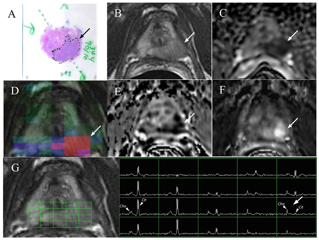
A 59 year-old male with serum PSA of 4.8 ng/ml and GS3+4 prostate cancer who underwent radical prostatectomy. a) H&E stained histology specimen, b) coil-corrected T2-weighted FSE image, c) ADC map, d) MRSI choline metabolite map, e) washout slope, f) maximal enhancement slope, g) magnetic resonance spectra with locations shown by the grid, Cit indicates the citrate peaks and Cho designates the choline peaks. The arrows designate cancerous lesions.

Figure 2:

A 56 year-old male with serum PSA of 12.5 ng/ml and GS4+3+5 prostate cancer who underwent radical prostatectomy. a) H&E stained histology specimen, b) coil-corrected T2-weighted FSE image, c) ADC map, d) MRSI choline metabolite map, e) washout slope, f) maximal enhancement slope. The arrows designate cancerous lesions.

Figure 3 summarizes the distribution of values observed for the imaging parameters in benign tissues, as well as in ≤GS3+3, in GS3+4, and in those GS4+3 and higher cancer tissues (≥GS4+3) in the peripheral zone. To determine the discriminatory value of each measured imaging parameter independent of each other, values obtained for each tissue and tumor type were compared. Within the peripheral zone, statistically significant differences were noted between benign and ≤GS3+3, benign and GS3+4, as well as benign and ≥GS4+3 for all imaging parameters. Additionally, statistically significant differences were noted between ≤GS3+3 and ≥GS4+3 on ADC (p=0.006), maximal enhancement slope (p=0.026), washout slope (p=0.0075), Cho/Cit ratio (p=0.0002), Cho/Cre (p<0.0001), and [Cho+Cre]/Cit (p=0.0013). Statistical significant differences were also noted between ≤GS3+3 and GS3+4 groups on washout slope (p=0.043) and Cho/Cre (p=0.02). MRSI-derived measures were the only parameters for which statistically significant differences were observed between GS3+4 and ≥GS4+3 cancers: Cho/Cre (p=0.031), Cho/Cit (p=0.028), and Cho+Cre/Cit (p=0.027).

Figure 3:

Box-plots comparing MR measures in normal peripheral zone tissues and ≤GS3+3, GS3+4, and ≥GS4+3 peripheral zone cancers. A) T2-weighted intensity, B) ADC, C) Peak Enhancement, D) Maximal Enhancement Slope, E) Washout Slope F) K^trans, G) Choline/Citrate, H) Choline/Creatine. Horizontal lines within the box plots represent the median values. Whiskers are drawn to the furthest points within 1.5x interquartile range, where interquartile range is the difference between the 1^st and the 3^rd quartiles.

*** <0.0001, ** <0.01, * <0.05

Figure 4 summarizes the distribution of values observed for the imaging parameters in benign tissues, as well as ≤GS3+3, GS3+4, and ≥GS4+3 cancers in the transition zone. Within the transition zone, statistically significant differences between benign and ≤GS3+3, benign and GS3+4, as well as benign and ≥GS4+3 cancers were noted on the majority of modalities as depicted in Figure 4. Additionally, statistically significant differences were observed between ≤GS3+3 and ≥GS4+3 groups on washout slope (p=0.0047), maximal enhancement slope (p=0.0422), and K^trans (p=0.0253). Statistically significant differences were also noted between ≤GS3+3 and GS3+4 cancers on ADC (p=0.0162), washout slope (p=0.0328), maximal enhancement slope (p=0.0328), and Cho/Cre (p=0.0111). No statistically significant differences were observed between GS3+4 and ≥GS4+3 cancers.

Figure 4:

Box-plots comparing MR measures in normal transition zone tissues and ≤GS3+3, GS3+4, and ≥GS4+3 peripheral zone cancers. A) T2-weighted intensity, B) ADC, C) Maximal Enhancement Slope, D) Washout Slope, E) k_ep, F) K^trans, G) Choline/Citrate, H) Choline/Creatine. Horizontal lines within the box plots represent the median values. Whiskers are drawn to the furthest points within 1.5x interquartile range, where interquartile range is the difference between the 1^st and the 3^rd quartiles.

*** <0.0001, ** <0.01, * <0.05

The results for the logistic regression analyses to discriminate between tissue types including the AUC, the specificity, and the sensitivity, are given in Tables 2 and 3. The results for the peripheral zone are summarized in Table 2, while Table 3 contains the results for the transition zone. The results of the repeated k-fold cross-validation of the combined models are summarized in Table 4, with the training and the validation ROC AUC, as well as the confidence intervals reported.

Table 2:

Peripheral zone – results of the logistic regression analysis with the area under the curve (AUC), sensitivity and specificity values demonstrating the capabilities of individual metric and combinations of parameters (listed in order of significance) to discriminate tissues of interest.

Parameter	Benign/All Cancers			≤G3+3/≥G3+4			≤G3+4/≥G4+3
	AUC	Sensitivity	Specificity	AUC	Sensitivity	Specificity	AUC	Sensitivity	Specificity
T2-weighted	0.74	55.2	90.8	0.52	35.5	78.7	0.55	46.8	71.4
ADC	0.94	84.5	89.2	0.69	61.3	76.6	0.67	80.9	54.3
Peak Enhancement (PE)	0.72	77.6	58.5	0.57	64.5	55.3	0.50	29.8	82.9
Max Enhancement Slope (ES)	0.80	70.7	80.0	0.65	74.2	57.5	0.59	63.8	62.9
Washout Slope (WO)	0.75	79.3	61.5	0.67	90.3	53.2	0.62	70.2	60.0
Ktrans	0.74	86.2	58.5	0.60	38.7	83.0	0.56	63.8	54.3
kep	0.71	91.4	46.2	0.58	61.3	58.7	0.56	89.4	34.3
vl	0.67	72.4	61.5	0.55	64.5	53.2	0.50	66.0	42.9
Choline (Cho)	0.55	44.8	81.5	0.68	67.7	70.2	0.63	55.3	80.0
Citrate (Cit)	0.82	60.3	96.9	0.62	80.7	61.7	0.72	66.0	74.3
Creatine (Cre)	0.74	58.6	90.8	0.61	83.9	53.2	0.73	66.0	77.1
Choline/Citrate (CC)	0.97	87.9	100	0.65	67.7	70.2	0.68	68.1	68.6
[Choline+Creatine]/Citrate (CCC)	0.96	87.9	95.4	0.62	71.0	63.8	0.64	48.9	80.0
Choline/Creatine (Cho/Cre)	0.99	94.8	98.5	0.68	64.5	74.5	0.74	59.6	85.7
Combined (Cho/Cre, ADC)	1	98.5	98.3
Combined (Cho, ES, ADC, Cit)				0.84	76.6	87.1
Combined (Cre, Cho, WO)							0.81	71.4	78.7

Table 3:

Transition zone – results of the logistic regression analysis with the area under the curve (AUC), sensitivity and specificity values demonstrating the capabilities of individual metric and combinations of parameters (listed in order of significance ) to discriminate tissues of interest.

Parameter	Benign/All Cancers			≤G3+3/≥G3+4			≤G3+4/≥G4+3
	AUC	Sensitivity	Specificity	AUC	Sensitivity	Specificity	AUC	Sensitivity	Specificity
T2-weighted	0.77	58.3	87.5	0.57	66.7	53.3	0.54	36.4	88.9
ADC	0.91	69.4	100.0	0.74	72.2	73.3	0.62	81.8	55.6
Peak Enhancement (PE)	0.56	58.3	58.3	0.59	44.4	80.0	0.58	45.5	77.8
Max Enhancement Slope (ES)	0.68	47.2	91.7	0.69	50.0	86.7	0.67	63.6	66.7
Washout Slope (WO)	0.67	97.2	37.5	0.76	77.8	73.3	0.69	68.2	77.8
Ktrans	0.66	91.7	37.5	0.74	83.3	66.7	0.71	68.2	77.8
kep	0.66	88.6	45.8	0.68	66.7	73.3	0.70	90.9	55.6
vl	0.50	38.9	70.8	0.57	83.3	40.0	0.60	63.6	66.7
Choline (Cho)	0.56	47.2	83.3	0.60	61.1	73.3	0.69	50.0	100
Citrate (Cit)	0.80	75.0	75.0	0.61	50.0	93.3	0.64	40.9	100
Creatine (Cre)	0.77	61.1	87.5	0.65	61.1	73.3	0.70	54.6	88.9
Choline/Citrate (CC)	0.94	94.4	91.7	0.40	22.2	93.3	0.55	59.1	66.7
[Choline+Creatine]/Citrate (CCC)	0.89	77.8	91.7	0.46	22.2	100.0	0.55	27.3	100.0
Choline/Creatine (Cho/Cre)	0.97	86.1	95.8	0.73	72.2	86.7	0.55	40.9	77.8
Combined (Cho/Cre, ADC)	0.99	100	91.7
Combined (WO, ADC, Cre)				0.93	86.7	94.4
Combined (Cho, WO)							0.92	77.8	100

Table 4:

The area under the curve (AUC) and the confidence intervals (CI) reported for the training and the validation models using the repeated 4-fold cross validation.

Region	Model	Benign/All Cancers			≤G3+3/≥G3+4			≤G3+4/≥G4+3
		AUC	95% CI		AUC	95% CI		AUC	95% CI
Peripheral Zone	Training	0.999 (± 0.001)	0.998	0.999	0.853 (± 0.026)	0.834	0.872	0.802 (± 0.030)	0.781	0.824
	Validation	0.993 (± 0.014)	0.983	1.003	0.777 (± 0.081)	0.719	0.835	0.793 (± 0.085)	0.732	0.854
Transition Zone	Training	0.991 (± 0.003)	0.989	0.993	0.935 (± 0.023)	0.919	0.951	0.926 (± 0.030)	0.905	0.948
	Validation	0.989 (± 0.012)	0.981	0.998	0.905 (± 0.080)	0.848	0.962	0.874 (± 0.132)	0.773	0.975

Appendices B and C summarize the results of the logistic regression analyses outlining AUC, sensitivity and specificity values for discriminating between tissue types for models derived using varying acquisition modalities. Figures 5A and 5B present receiver operating characteristic (ROC) curves for models in the peripheral and transition zones respectively, visually demonstrating the performance of each model and the contributions due to individual modalities in distinguishing ≤GS3+3 and ≥GS3+4 cancers.

Figure 5:

ROC curves demonstrating the performance of logistic regression models in distinguishing ≤GS3+3 and ≥GS3+4 cancers with varying combinations of acquired imaging modalities within A) the peripheral zone and B) the transition zone.

4. Discussion

Using one or a combination of several quantitative parameters derived from MR imaging to separate benign tissues from PCa and discriminate among different levels of PCa aggressiveness is a promising step toward improving prostate cancer characterization. A few studies have reported on the associations of individual imaging parameters and prostate Gleason grading.^9–14,17 For instance, Wang et al. found statistically significant associations between higher Gleason scores and lower tumor to muscle signal intensity ratio on T2-weighted images.⁹ Statistically significant negative correlations were reported between diffusion ADC values and prostate cancer Gleason scores.^10–13 Studies such as ACRIN have raised questions regarding suitability of spectroscopy for cancer detection, particularly for smaller ≤GS3+3 lesions²⁵; however, despite this limitation, MRSI has been shown an excellent technique for cancer characterization.^14,15,26 The combinations of different metabolite ratios i.e. choline plus creatine to citrate, choline to citrate, or choline/creatine obtained from MRSI shows promise for discrimination of low-grade and higher-grade prostate tumors.^14,15,26 Several studies have also reported promising associations between DCE MRI derived parameters and Gleason grades.^11,16,17 Chen et al observed a statistically significant association between the washout gradient and Gleason scores.¹⁶ Peng et al noted moderate correlations of K^trans with Gleason scores¹¹, while Vos et al found that a combination of DCE MRI parameters (mean and 75th percentile values of enhancement slope, mean washout, and 75th percentile values of K^trans) may aid in separating low-risk from more aggressive cancers.¹⁷ In the last few years, several groups have published predictive models obtained by considering sets of predictors made up of multiple imaging parameters.^11,27,28 Unfortunately, some studies are limited by the use of biopsy-based histopathology²⁷, which is associated with sampling errors.⁵ Others, while using prostatectomy histopathology for imaging validation, performed an abbreviated imaging protocol, resulting in incomplete multiparametric models.¹¹ Additionally, most studies exclude lesions smaller than 0.5cc.^28,29 Such size restrictions may limit applicability of the findings to the growing active surveillance patient population.

This study examined all imaging modalities currently available in clinical scanning and used post-radical prostatectomy whole mount histopathology as the reference standard. To identify the purest cancer signatures, we only looked at regions with homogeneous imaging appearance. Unlike other studies, our cancer size restrictions were minimal. We included all regions of interest greater than 0.05cc, with resultant median cancer lesion-based ROI size of 0.30cc in the peripheral zone and 0.28cc in the transition zone, with lesion sizes ranging from 0.05cc to 8.28cc and 0.05cc to 2.05cc for the two regions respectively.

Within the peripheral zone, while statistically significant differences between benign and malignant tissues were observed for all imaging parameters, logistic regression yielded the highest AUC values for Cho/Cre and ADC. A combination of these parameters resulted in a complete separation of benign and malignant tissues with an AUC of 1.0. The stability of the model was demonstrated using repeated four-fold cross-validation, which yielded an AUC of 0.99 (95% confidence interval, 0.98 - 1). Similar results were seen in the transition zone by combining Cho/Cre ratio and ADC, which yielded an AUC of 0.99 with a validation AUC of 0.99 (95% confidence interval, 0.98 – 1.00), indicating the excellent performance of the model. Interestingly, Cho/Cre was the single best performing parameter for distinguishing benign and malignant tissues for both the peripheral zone and the transition zone, demonstrating AUC values of 0.99 and 0.97 respectively, higher than those observed for ADC. The excellent performance of the MRSI-derived metrics is likely due in part to the unique nature of the choline parameter, to the high quality of the acquired data (largely due to the use of the endorectal coil), and to the reduction of systematic acquisition artifacts by use of either a ratio of peaks or the metabolite intensity corrections that were done to account for the inhomogeneity of the endorectal coil reception profile. This excellent performance argues for continued utilization of MRSI for prostate characterization. These results are similar or better than those reported in literature: with AUC values for combined models for discrimination of normal and cancerous regions ranging from 0.82 to 0.96 in the peripheral zone^28,30,31 and 0.76 to 0.92 in the transition zone.^32–34 One reason for this is likely our definition of “normal” tissues and the homogeneous nature of our ROIs. By limiting benign tissues to normal tissues and cystic atrophy we likely observe higher AUC values than those expected if the atrophic tissues, inflammation, benign prostatic hyperplasia (in the TZ), etc. were included in the benign subset.

Next, the ability of mpMRI parameters to distinguish ≤GS3+3 from ≥GS3+4 prostatic cancers was investigated. Studies have noted the importance of identifying a Gleason 4 component in order to better monitor disease progression and minimize risk of prostate cancer specific mortality.³⁵ Within the peripheral zone a combination of choline, maximal enhancement slope, ADC, and citrate metabolites yielded an AUC of 0.84 with good sensitivity and specificity values of 76.6 and 87.1 respectively. This suggests that some of the ≤GS3+3 cancers tend to look more aggressive on imaging. This is not surprising since separating ≤GS3+3 and GS3+4 cancers with minimal Gleason 4 disease is a considerable challenge, and these aggressive appearing G3+3 tumors could be genetically³⁶ and metabolically³⁷ more aggressive leading to poorer outcomes. In the transition zone, a combination of washout slope, ADC, and creatine yielded an AUC of 0.93. This result highlights the importance of using a comprehensive mpMR imaging, incorporating both DCE and MRSI when assessing the aggressiveness of prostate cancer at diagnosis in a contemporary early stage population of patients.

Finally, in order to assess our ability to distinguish low-risk from high-risk disease, we examined the performance of mpMRI parameters at separating grouped ≤GS3+3 and GS3+4 cancers from ≥GS4+3 prostate lesions. At many institutions patients can continue with active surveillance in the presence of GS3+4 disease; however, diagnosis of GS4+3 cancers on biopsy typically triggers treatment with curative intent, which makes our ability to separate the two groups of clinical importance. Within the peripheral zone, a combination of creatine, choline, and washout slope yielded an AUC of 0.81 with a sensitivity of 71.4 and a specificity of 78.7, likely due to the considerable challenges associated with separating GS3+4 and GS4+3 lesions on imaging. While this separation is challenging, Gleason Score may not be the best indicator of risk. Some cases of GS3+4 disease may progress; those with large, conspicuous lesions on mpMRI, such as in the case in Figure 1, may be more worrisome. In the transition zone, combining choline and washout slope yielded an AUC of 0.92 for discriminating between ≤GS3+4 and ≥GS4+3 disease, with excellent sensitivity of 77.8 and a good specificity of 100. It is important to note that all the models described above had very narrow confidence intervals and excellent corresponding validation AUC values, indicating the robustness of the final models.

Other studies have looked at separating low and high-risk prostate cancers. In a 2015 study, Vos et al. reported a combined AUC of 0.85 for separating low-grade PCa (defined as GG ≤3) from high-grade lesions (defined as GG ≥4) in the peripheral zone and an AUC of 0.92 for the transition zone.²⁸ Peng et al. also looked at using combined models to distinguish low-grade disease (GS3+3) and high-grade lesions (GS 7, 8, 9) and reported an AUC of 0.77 for their combined model within the peripheral zone.¹¹ These and our models show promise in using an mpMRI technique for evaluation of cancer. Our models go a step further in showing the ability of mpMRI to discriminate low-risk from high-risk prostate cancers even for smaller lesions, which is critical in the setting of early stage disease typically found in active surveillance patients.

We also looked at the performance of logistic regression models in the setting of missing imaging modalities. There are circumstances in which some modalities are not acquired due to various contraindications or the acquired data is unusable. For instance, DCE is typically not acquired in patients with compromised kidney function; diffusion weighted images are often unusable in patients with hip replacements, while the quality of the MRSI data may be degraded due to susceptibility artifacts produced by fecal matter at the endorectal coil/prostate boundary.

Across all tissue types and prostate zones, the best discriminating abilities were associated with logistic regression models that included all the imaging modalities. When separating benign tissues from cancer, all models showed good to excellent performance. When only two imaging modalities were included, T2-weighted image intensity combined with DCE parameters had the lowest, albeit high, performance in both the PZ and the TZ with AUC values of 0.90 and 0.80 respectively (Appendices B, C). When separating ≤GS3+3 and ≥GS3+4 cancers, the presence of MRSI-derived measures within the LR models played an important role in both the PZ and TZ, while DCE-derived measures outperformed other modalities within the TZ models When discriminating ≤GS3+4 and ≥GS4+3 PCa, MRSI played a critical role within the constructed LR models with DCE and DWI-derived measures performing equally well within the PZ. Within the TZ, DCE and MRSI-derived parameters both played an important role in separating ≤GS3+4 and ≥GS4+3 cancers, with DWI-derived ADC values not contributing to the performance of the overall models.

The role of multiparametric MR imaging in prostate cancer management is continually evolving. T2-weighted imaging and DW imaging are universally accepted for PCa diagnosis. Version 1 of the Prostate Imaging – Reporting and Data System (PI-RADS) published in 2012 and designed to standardize acquisition, interpretation and reporting of mpMRI scans was based solely on T2-weighted imaging and DWI.³⁸ The current PI-RADS version 2 entirely omits MRSI and advises the use of qualitative DCE MRI only in cases of borderline findings on DWI and T2w imaging in the peripheral zone and omits the use of DCE MRI for detection of lesions in the transition zone. Our study showed the importance of both MRSI measurements and DCE MRI-derived quantitative parameters for building better models for discriminating between prostatic cancerous and benign tissues, and more importantly for distinguishing between malignant prostatic tissues of various grades. This suggests further advances to develop and translate DCE MRI and MRSI into widespread clinical use are warranted. These findings of excellent separation between tissues are important for improving therapeutic selection for individual patients, and for designing improved clinical trials of new therapeutic approaches.

Our study has several limitations. First, the regions of interest were manually drawn on MR images based on the histopathology; this approach could have potentially introduced bias toward outlining MR visible features as opposed to histologically evident cancers. Second, MR sequences were manually aligned to each other based upon visual assessment; however, it is possible that some regions were not perfectly transferred from one sequence to another. Third, this study only included cancer regions with homogeneous imaging appearance. This selection process resulted in smaller ROIs than the histopathological lesions and does introduce bias to our results. Fourth, prostate tissues are extremely heterogeneous; in the analysis above normal tissues and cystic atrophy were presented as benign tissues. This is an oversimplification of the complex nature of the benign prostatic tissues, which requires further exploration. High-b DW imaging was incorporated into the imaging protocol part way through the study. Due to low numbers (only 35/78 patients had high-b DW imaging performed), high-b DWI, which has proven to be very useful in contemporary studies,^39,40 was not included in the models. Finally, truth in this study was based solely on pathologic grade at surgery, mpMRI may be able to identify those GS3+3 tumors that could result in poor clinical outcomes.

5. Conclusion

This study demonstrated excellent separation of benign tissues and PCa, as well as cancers across Gleason Scores in the peripheral zone and in the transition zone using mpMRI, even in very small lesions. Quantitative measures of DWI, MRSI, and DCE MRI aided the discrimination between Gleason Grade groups of cancers, underlining the value of a comprehensive mpMRI protocol for evaluation of prostate cancer presence and aggressiveness.

Abbreviations:

ADC

apparent diffusion coefficient

AUC

area under the receiver operating characteristics curve

DCE

dynamic contrast-enhanced

DWI

diffusion weighted imaging

GS

Gleason Score

k_ep

rate constant between extracellular extravascular space and plasma space

K^trans

volume transfer constant

LR

logistic regression

MP

multiparametric

MRSI

magnetic resonance spectroscopic imaging

PCa

prostate cancer

PZ

peripheral zone

ROI

region of interest

TZ

transition zone

v_ees

fractional extravascular, extracellular volume

v_l

fractional luminal volume

Appendix A: Scanning parameters.

Imaging	PSD	TR/TE (ms)	FOV (cm)	Matrix Size	NEX	ST (mm)	In-Plane Res. (mm)	Temp. Res. (s)	b-value (s/mm2)
T2w	FSE	6000/100	18x18	512x512	1	3	0.35x0.35	N/A	N/A
Conv ADC	ss-EPI	4000/90	24x24	128x128	4	3	0.94x0.94	N/A	0, 600
rFOV ADC	ss=EPI	4000/90	18x9	128x64	6	3	0.70x0.70	N/A	0, 600
MRSI	3D PRESS	2000/85	varied	8x16	1	2.7	5.4x2.7	N/A	N/A
DCE	3D SPGR	3.5/0.9	26x26	256x256	0	3	1.02x1.02	10.417	N/A

PSD=pulse sequence design, ST= slice thickness, Res=resolution, T2w = T2-weighted MRI, Conv = conventional, rFOV=reduced FOV.

Appendix B: Peripheral zone: results of the logistic regression analysis with the area under the curve (AUC), sensitivity and specificity values demonstrating the importance of imaging modalities in discriminating tissues of interest. Parameters are listed from most significant to least significant within each set of modalities.

Benign vs. All Cancer
Modalities	Parameters	AUC	Sensitivity	Specificity
T2w, DWI	ADC	0.94	89.2	84.5
T2w, DCE	T2,Slope, kep	0.90	86.2	81.0
T2w, MRSI	Cho/Cre	0.99	98.5	84.8
T2, DWI, DCE	Slope, vl, ADC	0.96	90.8	89.7
T2, DCE, MRSI	Slope, Cho/Cre, CCC, vl, T2, Cho/Cit	1.00	100	100
T2, DWI, MRSI	ADC, Cho/Cre	1.00	98.5	98.3
All	Cho/Cre, ADC	1.0	98.5	98.3
≤G3+3 vs. ≥G3+4
Modalities	Parameters	AUC	Sensitivity	Specificity
T2w, DWI	ADC	0.69	76.6	61.3
T2w, DCE	Slope	0.65	57.5	74.2
T2w, MRSI	Cho, Cho/Cre	0.76	68.1	83.9
T2, DWI, DCE	ADC, Slope	0.73	63.8	77.4
T2, DCE, MRSI	Cho, Slope, Cit	0.80	63.8	87.1
T2, DWI, MRSI	Cho, ADC, Cit	0.79	78.7	74.2
All	Cho, ADC, Kep, Cit	0.83	76.6	80.6
≤G3+4 vs. ≥G4+3
Modalities	Parameters	AUC	Sensitivity	Specificity
T2w, DWI	ADC	0.67	54.3	80.8
T2w, DCE	WO	0.62	60.0	70.2
T2w, MRSI	Cre, Cho	0.77	80.0	66.0
T2, DWI, DCE	ADC, WO	0.69	48.6	87.2
T2, DCE, MRSI	Cre, Cho, WO	0.81	71.4	78.7
T2, DWI, MRSI	Cre, Cho, ADC	0.80	82.9	66.0
All	Cre, Cho, WO	0.81	71.4	78.7

Slope = maximal enhancement slope, WO = washout slope

Appendix C: Transition zone: results of the logistic regression analysis with the area under the curve (AUC), sensitivity and specificity values demonstrating the importance of imaging modalities in discriminating tissues of interest. Within each set of modalities, parameters are listed from most significant to least significant.

Benign vs. All Cancer
Modalities	Parameters	AUC	Sensitivity	Specificity
T2w, DWI	ADC, T2	0.93	100	83.3
T2w, DCE	T2, Slope	0.80	95.8	63.9
T2w, MRSI	Cho/Cre, T2	0.98	100	86.1
T2, DWI, DCE	ADC, T2	0.93	100	83.3
T2, DCE, MRSI	Cho/Cre, T2	0.98	100	86.1
T2, DWI, MRSI	Cho/Cre, ADC	0.99	100	91.7
All	Cho/Cre, ADC	0.99	100	91.7
≤G3+3 vs. ≥G3+4
Modalities	Parameters	AUC	Sensitivity	Specificity
T2w, DWI	ADC	0.74	73.3	72.2
T2w, DCE	WO, VL	0.80	93.3	61.1
T2w, MRSI	CCC, Cho/Cre, Cit	0.80	53.3	94.4
T2, DWI, DCE	WO, ADC, VL	0.89	86.7	83.3
T2, DCE, MRSI	WO, Cre	0.86	80.0	83.3
T2, DWI, MRSI	Cho/Cre, ADC, Cho/Cit, CCC	0.93	80.0	100
All	WO, ADC, Cre	0.93	86.7	94.4
≤G3+4 vs. ≥G4+3
Modalities	Parameters	AUC	Sensitivity	Specificity
T2w, DWI	ADC	0.62	55.6	81.8
T2w, DCE	Ktrans	0.71	77.8	68.2
T2w, MRSI	Cho	0.69	100	50
T2, DWI, DCE	Ktrans	0.71	77.8	68.2
T2, DCE, MRSI	Cho, WO	0.92	77.8	100
T2, DWI, MRSI	Cho	0.69	100	50
All	Cho, WO	0.92	77.8	100

PE = peak enhancement, Slope = maximal enhancement slope, WO = washout slope

References

- 1.Siegel RL, Miller KD, Jemal A. Cancer statistics, 2016. CA: a cancer journal for clinicians. 2016;66(1):7–30. [DOI] [PubMed] [Google Scholar]
- 2.Resnick MJ, Koyama T, Fan KH, et al. Long-term functional outcomes after treatment for localized prostate cancer. The New England journal of medicine. 2013;368(5):436–445. [DOI] [PMC free article] [PubMed] [Google Scholar]
- 3.Gustafsson O, Norming U, Almgard LE, et al. Diagnostic methods in the detection of prostate cancer: a study of a randomly selected population of 2,400 men. The Journal of urology. 1992;148(6):1827–1831. [DOI] [PubMed] [Google Scholar]
- 4.Epstein JI, Partin AW, Sauvageot J, Walsh PC. Prediction of progression following radical prostatectomy. A multivariate analysis of 721 men with long-term follow-up. Am J Surg Pathol. 1996;20(3):286–292. [DOI] [PubMed] [Google Scholar]
- 5.Serefoglu EC, Altinova S, Ugras NS, et al. How reliable is 12-core prostate biopsy procedure in the detection of prostate cancer? Cuaj-Can Urol Assoc. 2013;7(5-6):E293–E298. [DOI] [PMC free article] [PubMed] [Google Scholar]
- 6.Loeb S, Vellekoop A, Ahmed HU, et al. Systematic review of complications of prostate biopsy. European urology. 2013;64(6):876–892. [DOI] [PubMed] [Google Scholar]
- 7.Hoeks CM, Barentsz JO, Hambrock T, et al. Prostate cancer: multiparametric MR imaging for detection, localization, and staging. Radiology. 2011;261(1):46–66. [DOI] [PubMed] [Google Scholar]
- 8.Johnson LM, Turkbey B, Figg WD, Choyke PL. Multiparametric MRI in prostate cancer management. Nature reviews Clinical oncology. 2014;11(6):346–353. [DOI] [PMC free article] [PubMed] [Google Scholar]
- 9.Wang L, Mazaheri Y, Zhang J, et al. Assessment of biologic aggressiveness of prostate cancer: correlation of MR signal intensity with Gleason grade after radical prostatectomy. Radiology. 2008;246(1):168–176. [DOI] [PubMed] [Google Scholar]
- 10.Hambrock T, Somford DM, Huisman HJ, et al. Relationship between Apparent Diffusion Coefficients at 3.0-T MR Imaging and Gleason Grade in Peripheral Zone Prostate Cancer. Radiology. 2011;259(2):453–461. [DOI] [PubMed] [Google Scholar]
- 11.Peng YH, Jiang YL, Yang C, et al. Quantitative Analysis of Multiparametric Prostate MR Images: Differentiation between Prostate Cancer and Normal Tissue and Correlation with Gleason Score-A Computer-aided Diagnosis Development Study. Radiology. 2013;267(3):787–796. [DOI] [PMC free article] [PubMed] [Google Scholar]
- 12.Turkbey B, Shah VP, Pang Y, et al. Is apparent diffusion coefficient associated with clinical risk scores for prostate cancers that are visible on 3-T MR images? Radiology. 2011;258(2):488–495. [DOI] [PMC free article] [PubMed] [Google Scholar]
- 13.Vargas HA, Akin O, Franiel T, et al. Diffusion-weighted endorectal MR imaging at 3 T for prostate cancer: tumor detection and assessment of aggressiveness. Radiology. 2011;259(3):775–784. [DOI] [PMC free article] [PubMed] [Google Scholar]
- 14.Kobus T, Hambrock T, Hulsbergen-van de Kaa CA, et al. In vivo assessment of prostate cancer aggressiveness using magnetic resonance spectroscopic imaging at 3 T with an endorectal coil. European urology. 2011;60(5):1074–1080. [DOI] [PubMed] [Google Scholar]
- 15.Zakian KL, Sircar K, Hricak H, et al. Correlation of proton MR spectroscopic imaging with Gleason score based on step-section pathologic analysis after radical prostatectomy. Radiology. 2005;234(3):804–814. [DOI] [PubMed] [Google Scholar]
- 16.Chen YJ, Chu WC, Pu YS, et al. Washout gradient in dynamic contrast-enhanced MRI is associated with tumor aggressiveness of prostate cancer. Journal of magnetic resonance imaging : JMRI. 2012;36(4):912–919. [DOI] [PubMed] [Google Scholar]
- 17.Vos EK, Litjens GJ, Kobus T, et al. Assessment of prostate cancer aggressiveness using dynamic contrast-enhanced magnetic resonance imaging at 3 T. European urology. 2013;64(3):448–455. [DOI] [PubMed] [Google Scholar]
- 18.Korn N, Kurhanewicz J, Banerjee S, et al. Reduced-FOV excitation decreases susceptibility artifact in diffusion-weighted MRI with endorectal coil for prostate cancer detection. Magnetic resonance imaging. 2015;33(1):56–62. [DOI] [PMC free article] [PubMed] [Google Scholar]
- 19.Chen AP, Cunningham CH, Ozturk-Isik E, et al. High-speed 3T MR spectroscopic imaging of prostate with flyback echo-planar encoding. Journal of magnetic resonance imaging : JMRI. 2007;25(6):1288–1292. [DOI] [PubMed] [Google Scholar]
- 20.Noworolski SM, Reed GD, Kurhanewicz J, Vigneron DB. Post-processing correction of the endorectal coil reception effects in MR spectroscopic imaging of the prostate. Journal of magnetic resonance imaging : JMRI. 2010;32(3):654–662. [DOI] [PMC free article] [PubMed] [Google Scholar]
- 21.Noworolski SM, Henry RG, Vigneron DB, Kurhanewicz J. Dynamic contrast-enhanced MRI in normal and abnormal prostate tissues as defined by biopsy, MRI, and 3D MRSI. Magnetic resonance in medicine. 2005;53(2):249–255. [DOI] [PubMed] [Google Scholar]
- 22.Tofts PS, Kermode AG. Measurement of the blood-brain barrier permeability and leakage space using dynamic MR imaging. 1. Fundamental concepts. Magnetic resonance in medicine. 1991;17(2):357–367. [DOI] [PubMed] [Google Scholar]
- 23.Noworolski SM, Reed GD, Kurhanewicz J. A Novel Luminal Water Model for DCE MRI of Prostatic Tissues. Paper presented at: International Society for Magnetic Resonance in Medicine 2011; Montreal. [Google Scholar]
- 24.R: A language and environment for statistical computing [computer program]. Vienna, Austria: R Foundation for Statistical Computing; 2015. [Google Scholar]
- 25.Weinreb JC, Blume JD, Coakley FV, et al. Prostate cancer: sextant localization at MR imaging and MR spectroscopic imaging before prostatectomy--results of ACRIN prospective multi-institutional clinicopathologic study. Radiology. 2009;251(1):122–133. [DOI] [PMC free article] [PubMed] [Google Scholar]
- 26.Giusti S, Caramella D, Fruzzetti E, et al. Peripheral zone prostate cancer. Pre-treatment evaluation with MR and 3D (1)H MR spectroscopic imaging: correlation with pathologic findings. Abdominal imaging. 2010;35(6):757–763. [DOI] [PubMed] [Google Scholar]
- 27.Dwivedi DK, Kumar R, Bora GS, et al. Stratification of the aggressiveness of prostate cancer using pre-biopsy multiparametric MRI (mpMRI). NMR in biomedicine. 2016;29(3):232–238. [DOI] [PubMed] [Google Scholar]
- 28.Vos EK, Kobus T, Litjens GJ, et al. Multiparametric Magnetic Resonance Imaging for Discriminating Low-Grade From High-Grade Prostate Cancer. Investigative radiology. 2015;50(8):490–497. [DOI] [PubMed] [Google Scholar]
- 29.Fehr D, Veeraraghavan H, Wibmer A, et al. Automatic classification of prostate cancer Gleason scores from multiparametric magnetic resonance images. Proc Natl Acad Sci USA. 2015;112(46):E6265–6273. [DOI] [PMC free article] [PubMed] [Google Scholar]
- 30.Liu L, Tian Z, Zhang Z, Fei B. Computer-aided Detection of Prostate Cancer with MRI: Technology and Applications. Academic radiology. 2016;23(8):1024–1046. [DOI] [PMC free article] [PubMed] [Google Scholar]
- 31.Niaf E, Rouviere O, Mege-Lechevallier F, Bratan F, Lartizien C. Computer-aided diagnosis of prostate cancer in the peripheral zone using multiparametric MRI. Physics in medicine and biology. 2012;57(12):3833–3851. [DOI] [PubMed] [Google Scholar]
- 32.Dikaios N, Alkalbani J, Sidhu HS, et al. Logistic regression model for diagnosis of transition zone prostate cancer on multi-parametric MRI. European radiology. 2015;25(2): 523–532. [DOI] [PMC free article] [PubMed] [Google Scholar]
- 33.Hambrock T, Vos PC, Hulsbergen-van de Kaa CA, Barentsz JO, Huisman HJ. Prostate cancer: computer-aided diagnosis with multiparametric 3-T MR imaging--effect on observer performance. Radiology. 2013;266(2):521–530. [DOI] [PubMed] [Google Scholar]
- 34.Hoeks CM, Hambrock T, Yakar D, et al. Transition zone prostate cancer: detection and localization with 3-T multiparametric MR imaging. Radiology. 2013;266(1):207–217. [DOI] [PubMed] [Google Scholar]
- 35.Lavery HJ, Droller MJ. Do Gleason Patterns 3 and 4 Prostate Cancer Represent Separate Disease States? The Journal of urology. 2012;188(5):1667–1675. [DOI] [PubMed] [Google Scholar]
- 36.Klein EA, Cooperberg MR, Magi-Galluzzi C, et al. A 17-gene assay to predict prostate cancer aggressiveness in the context of Gleason grade heterogeneity, tumor multifocality, and biopsy undersampling. European urology. 2014;66(3):550–560. [DOI] [PubMed] [Google Scholar]
- 37.Priolo C, Pyne S, Rose J, et al. AKT1 and MYC induce distinctive metabolic fingerprints in human prostate cancer. Cancer research. 2014;74(24):7198–7204. [DOI] [PMC free article] [PubMed] [Google Scholar]
- 38.Barentsz JO, Weinreb JC, Verma S, et al. Synopsis of the PI-RADS v2 Guidelines for Multiparametric Prostate Magnetic Resonance Imaging and Recommendations for Use. European urology. 2016;69(1):41–49. [DOI] [PMC free article] [PubMed] [Google Scholar]
- 39.Kitajima K, Takahashi S, Ueno Y, et al. Clinical utility of apparent diffusion coefficient values obtained using high b-value when diagnosing prostate cancer using 3 tesla MRI: comparison between ultra-high b-value (2000 s/mm(2)) and standard high b-value (1000 s/mm(2)). Journal of magnetic resonance imaging : JMRI. 2012;36(1):198–205. [DOI] [PubMed] [Google Scholar]
- 40.Ueno Y, Kitajima K, Sugimura K, et al. Ultra-high b-value diffusion-weighted MRI for the detection of prostate cancer with 3-T MRI. Journal of magnetic resonance imaging : JMRI. 2013;38(1):154–160. [DOI] [PubMed] [Google Scholar]