

Abstract
The Scientific Committee (SC) reconfirms that the benchmark dose (BMD) approach is a scientifically more advanced method compared to the no‐observed‐adverse‐effect‐level (NOAEL) approach for deriving a Reference Point (RP). The major change compared to the previous Guidance (EFSA SC, 2017) concerns the Section 2.5, in which a change from the frequentist to the Bayesian paradigm is recommended. In the former, uncertainty about the unknown parameters is measured by confidence and significance levels, interpreted and calibrated under hypothetical repetition, while probability distributions are attached to the unknown parameters in the Bayesian approach, and the notion of probability is extended to reflect uncertainty of knowledge. In addition, the Bayesian approach can mimic a learning process and reflects the accumulation of knowledge over time. Model averaging is again recommended as the preferred method for estimating the BMD and calculating its credible interval. The set of default models to be used for BMD analysis has been reviewed and amended so that there is now a single set of models for quantal and continuous data. The flow chart guiding the reader step‐by‐step when performing a BMD analysis has also been updated, and a chapter comparing the frequentist to the Bayesian paradigm inserted. Also, when using Bayesian BMD modelling, the lower bound (BMDL) is to be considered as potential RP, and the upper bound (BMDU) is needed for establishing the BMDU/BMDL ratio reflecting the uncertainty in the BMD estimate. This updated guidance does not call for a general re‐evaluation of previous assessments where the NOAEL approach or the BMD approach as described in the 2009 or 2017 Guidance was used, in particular when the exposure is clearly lower (e.g. more than one order of magnitude) than the health‐based guidance value. Finally, the SC firmly reiterates to reconsider test guidelines given the wide application of the BMD approach.
Keywords: BMD, BMDL, benchmark response, NOAEL, dose–response modelling, BMD software, Bayesian model averaging
Short abstract
This publication is linked to the following EFSA Supporting Publications article: http://onlinelibrary.wiley.com/doi/10.2903/sp.efsa.2022.EN-7585/full
Summary
Considering the need for transparent and scientifically justifiable approaches to be used when risks are assessed by the Scientific Committee (SC) and the Scientific Panels of EFSA, the SC was requested in 2005 by EFSA (i) to assess the existing information on the utility of the benchmark dose (BMD) approach, as an alternative to the traditionally used no‐observed‐adverse‐effect‐level (NOAEL) approach; (ii) to provide guidance on how to use the BMD approach for analysing dose–response data from experimental animal studies; and (iii) to look at the possible application of this approach to data from observational epidemiological studies.
A guidance document on the use of the benchmark dose approach in risk assessment was published in 2009. In 2015, the SC reviewed the implementation of the BMD approach in EFSA's work, the experience gained with its application and the latest methodological developments in regulatory risk assessment and concluded that an update of its guidance from 2009 was necessary. As a consequence, an updated guidance document was published in 2017. Most of the modifications made at the time concerned the section providing guidance on how to apply the BMD approach in practice. Model averaging was recommended as the preferred method for calculating the BMD confidence interval, while acknowledging that the respective tools were still under development.
Following a workshop organised by EFSA in March 2017 to discuss commonalities and divergences in the various approaches for BMD analysis worldwide, and the update of the Chapter 5 on dose–response assessment of WHO/IPCS Environmental Health Criteria 240 (WHO, 2020), the SC decided to update again its guidance in order to align the content of the document with internationally agreed concepts related to benchmark dose analysis, and therefore harmonise further EFSA's approach with those of its partners. The major change to the update of the SC Guidance of 2017 concerns the Section 2.5, in which a change from the frequentist to the Bayesian paradigm is recommended. In the former, uncertainty about the unknown parameters was measured by confidence and significance levels, interpreted and calibrated under hypothetical repetition, while probability distributions are attached to the unknown parameters in the Bayesian approach, and the notion of probability is extended so that it reflects uncertainty of knowledge. In addition, the Bayesian approach can mimic a learning process and reflects the accumulation of knowledge over time. Model averaging is again recommended as the preferred method for calculating the BMD credible interval. The set of default models to be used for BMD analysis has been reviewed and amended so that there is now a single set of models for both quantal and continuous data. The flow chart guiding the reader step‐by‐step when performing a BMD analysis has also been updated, and a chapter comparing the frequentist to the Bayesian paradigm inserted. Also, when using Bayesian BMD modelling, the potential Reference Point (RP) is provided by the lower bound (BMDL) of the credible interval, and the upper bound (BMDU) is needed for establishing the BMDU/BMDL ratio, which reflects the uncertainty around the BMD estimate.
The SC reconfirms in the present updated guidance that the BMD approach, and more specifically model averaging, should be used for deriving a RP from the critical dose–response data to establish health‐based guidance values (HBGVs) and margins of exposure. This updated guidance does not call for a general re‐evaluation of previous assessments where the NOAEL approach or the BMD approach as described in the 2009 or 2017 SC Guidance was used, in particular when the exposure is clearly smaller (e.g. more than one order of magnitude) than the HBGV. The application of this updated guidance to previous risk assessments where the 2009 or 2017 guidance was used might result in different RPs, in particular in the case of continuous response data where informative priors are used.
The SC recommends that training in dose–response modelling and the use of the BMD application hosted in the R4EU servers continues to be offered to experts in the Scientific Panels and EFSA Units. Furthermore, the option for the Cross‐Cutting Working Group on BMD analysis to be consulted by EFSA experts and staff if needed, should be maintained.
Finally, the SC firmly reiterates the need for current toxicity test guidelines to be reconsidered given the wide application of the BMD approach, as well as the need for a specific guidance on the use of the BMD approach to analyse human data.
1. Background
As per EFSA's Founding Regulation (EC) No 178/2002 of the European Parliament and of the Council, ‘the EFSA Scientific Committee shall be responsible for the general coordination necessary to ensure the consistency of the scientific opinion procedure, in particular with regard to the adoption of working procedures and harmonisation of working methods’. Strategic objective 2 of the EFSA Strategy 2027 regarding ensuring preparedness for future risk analysis needs echoes this key responsibility of the Scientific Committee, putting the emphasis on the development of a harmonised risk assessment culture and the improvement of the assessment methodologies to address future challenges.
In May 2009, the Scientific Committee adopted its guidance on the use of the benchmark dose (BMD) approach in risk assessment (EFSA, 2009). The guidance document recommends using the BMD approach instead of the traditionally used NOAEL approach to identify a Reference Point, since it makes a more extended use of dose–response data and allows for a quantification of the uncertainties in the dose–response data. In principle, the BMD approach is applicable to all chemicals for which a dose–response relationship exists for at least one endpoint, irrespective of their category (e.g. pesticide, food additive, contaminant) or origin (chemically synthesised or from natural sources). Within the remit of EFSA, this guidance document addresses the assessment of substances in food. The guidance was further updated in 2017 (EFSA Scientific Committee, 2017), recommending model averaging as the preferred approach for BMD analysis; the set of mathematical models to be fitted to the data by default was updated, and a flow chart, guiding step‐by‐step the reader when performing BMD analysis was added.
Following a workshop organised by EFSA in March 2017 to discuss commonalities and divergences in the various approaches for BMD analysis worldwide,1 WHO convened a group of experts from all over the world to update Chapter 5 on dose–response assessment of WHO/IPCS Environmental Health Criteria 240 (WHO, 2020). This work resulted in a consensus on a number of concepts related to benchmark dose analysis.
The purpose of the present update of the EFSA Guidance on the use of the benchmark dose approach in risk assessment is to align the content of the document with the above‐mentioned agreed concepts, and therefore harmonise further EFSA's approach with those of its partners.
1.1. Terms of Reference as provided by EFSA
The European Food Safety Authority requests the Scientific Committee to align the Guidance on the use of the benchmark dose approach in risk assessment with the principles for dose–response assessment described in chapter 5 of FAO/WHO IPCS EHC2402. EFSA Partners (US EPA, US NIOSH, US FDA, Health Canada, EU Member States competent authorities, EFSA Sister Agencies and other international partners) will be involved/consulted during the drafting phase.3
EFSA is requesting its Assessment Methodology (AMU) Unit to update its Platform for BMD analysis so that it implements the above‐mentioned updated guidance on BMD.4 When doing so, harmonisation with other existing BMD tools (US EPA BMDS and PROAST) will be sought.
1.2. Interpretation of Terms of Reference
To address the mandate received, the following modifications have been made to the 2017 SC Guidance on the use of the benchmark dose approach in risk assessment:
The extension and unification of the suite of models for continuous and quantal endpoints (Sections 2.5.1 and 2.5.2),
Introduction of the normal distribution, next to the Log‐normal distribution default assumption of the response at a specified dose level for continuous endpoints (Section 2.5.1).
The introduction of the Bayesian inferential paradigm and the rationale for replacing the Frequentist BMD model averaging by the Bayesian model averaging as the recommended preferred approach to estimate the BMD and calculate its credible5 interval (Section 2.5.3).
Guidance on how to select the Benchmark Response (Section 2.6.2).
Guidance on how to decide whether experimental data are worth modelling and if not, recommendation on how to use these data for the assessment (Section 2.6.3).
Guidance on how to construct informative priors (Section 2.6.4).
Guidance on how to deal with data leading to unpractical BMDLs and/or large BMDL‐BMDU credible intervals (Section 2.6.5).
Guidance on how to perform BMD analysis on data sets with no non‐exposed controls (Section 2.6.3).
Guidance on how to handle high dose impact (Section 2.6.3).
This document updates the methodology used by EFSA to perform BMD analysis; an online application is being developed that aligns with this guidance. A separate technical report6 describing in detail the framework, as well as a user guide for the application, are being developed.
2. Assessment
2.1. Introduction
This Guidance is an update and modification of the version released in 2017 (EFSA SC, 2017). The purpose of this update is to further support the implementation of dose–response modelling in EFSA's work and to harmonise the statistical background and theoretical insights between EFSA and other national and international organisations such as WHO (EHC240 Chapter 5 (WHO, 2020)) and US EPA (2012).
This document addresses the analysis of dose–response data from toxicity studies in experimental animals. Toxicity studies are conducted to identify and characterise potential adverse effects of a substance. The data obtained in these studies may be further analysed to identify a dose that can be used as a starting point for risk assessment. The dose used for this purpose, however derived, is referred to in this opinion as the Reference Point (RP). This term, adopted by the EFSA in 2005 (EFSA, 2005a) is preferred to the equivalent term Point of Departure (PoD), used by others such as US EPA.
The no‐observed‐adverse‐effect‐level (NOAEL) has been used historically as the RP for establishing health‐based guidance values (HBGVs) in risk assessment of non‐genotoxic substances. EFSA (2005a) and the Joint FAO/WHO Expert Committee on Food Additives (JECFA, 2006a) have proposed the use of the benchmark dose (BMD) approach for deriving RPs used to calculate the margins of exposure (MOEs) for substances that are both genotoxic and carcinogenic, since for such substances it is conventionally considered inappropriate to identify NOAELs for use as RPs.
The SC concluded in 2009 that the BMD approach is the preferred approach for identifying a RP; not only for substances that are both genotoxic and carcinogenic, but also for non‐genotoxic substances (EFSA, 2009; EFSA SC, 2017). The methodology discussed in the 2009 guidance document and its update from 2017 has increasingly been applied by EFSA for identifying RPs (i.e. BMDLs) for various types of chemicals (e.g. pesticide, additives and contaminants).
In Sections 2.3.1 and 2.3.2 of this guidance document, the concepts underlying both the NOAEL and BMD approaches are briefly discussed (see EFSA, 2009 for more details), and it is outlined why the SC considers the BMD approach a more powerful approach. Section 2.4 discusses the potential impact of using the BMD approach for hazard/risk characterisation and risk communication. Within EFSA, the main application of the BMD approach is to identify a RP for a chemical hazard (hazard characterisation) and subsequently – based on exposure data – characterise the chemical risk (risk characterisation). The SC notes that the BMD approach has also been used for other purposes such as for evaluating the plausibility of non‐monotonicity in a dose–response curve (parameter d is a measure of the steepness of the curve, Beausoleil et al., 2016) or for estimating relative potencies of chemicals (e.g. organophosphates, Bosgra et al., 2009 or Zeilmaker et al., 2018). However, these applications of the BMD approach are outside the scope of the present Guidance.
Further, the set of default models to be used for BMD analysis has been revised; they are described in Sections 2.5.1 and 2.5.2. The Bayesian model averaging procedure, recommended as the preferred approach for BMD analysis, is described in Section 2.5.3 and in later sections possible extensions on how to incorporate covariates and deal with cluster data in the analysis are covered. In Appendces C and D, examples based on continuous and quantal data are provided to illustrate the application of the BMD approach in practice and a discussion of the results is presented. A template for BMD analysis reporting has been inserted in Appendix E.
Section 2.6, which provides guidance on how to apply the BMD approach in practice, has been significantly modified compared to the 2009 and 2017 versions of the guidance document: Bayesian model averaging has been introduced as the preferred method for estimating the BMD and calculating its credible interval. The problem formulation step has been particularly expanded, providing further guidance on key decisions to be taken before starting to model the data: specification of the BMR, data suitability to estimate the BMD using dose–response modelling, consideration of prior information for the endpoint(s) considered.
The principles outlined in this guidance document may also apply to data from (observational) epidemiological studies. However, such studies have their own peculiarities with respect to study design and interpretation of data and for these reasons, the application of dose–response analysis of epidemiological data will be addressed in a separate future guidance document. Furthermore, this Guidance has not been developed for application to ecotoxicological studies/data. However, the method is sufficiently generic that it could reasonably be applied to other areas, as long as the dose–response is monotonic and a critical effect is defined in terms of relative change compared to the background response.
The present guidance is primarily aimed at EFSA Units and Panels and other stakeholders, for example applicants, performing dose–response analyses. The SC considers that the use of the BMD approach is the preferred approach compared to the NOAEL approach to identify a RP; therefore, the application of this guidance document is unconditional for EFSA and is strongly recommended for all parties submitting assessments to EFSA for peer‐review or dossiers for authorisation purposes (see EFSA Scientific Committee, 2015).
2.2. Hazard identification: selection of potential critical endpoints
Toxicity studies are designed to identify adverse effects produced by a substance, and to characterise the dose–response relationships for the adverse effects detected. While human dose–response data are occasionally available, most risk assessments rely on data from animal studies. The aim of hazard identification is to identify potential critical endpoints that may be of relevance for human health. An important component in hazard identification is the consideration of dose dependency of observed effects. Traditionally this is done by visual inspection together with conventional statistical tools. Dose–response modelling approaches (see Section 2.5) can also be used to support the evaluation. When no statistical evidence for a treatment‐related change is observed, the data set for the endpoint under consideration would normally not be used for identifying an RP. The selection of any critical adverse effect should not solely be based on statistical procedures and considerations of its biological relevance for human risk assessment are key (see also Section 2.6.2). Importantly, additional toxicological considerations should be taken into account in the evaluation of a toxicological data package. Use of the BMD approach does not remove the need for a critical evaluation of the response data7 and an assessment of the relevance of the effect to human health.
2.3. Using dose–response data in hazard characterisation
In the hazard characterisation, the nature of the dose–response5 relationships is explored in detail. The overall aim of the process is to identify a dose (the RP) from the toxicity studies that will then be used to establish a level of human intake at which it is confidently expected that there would be no appreciable adverse health effects, taking into account uncertainty and variability such as inter‐ and intraspecies differences, suboptimal study characteristics or missing data.
Hazard characterisation in risk assessment requires the use of a range of dose levels in toxicity studies. Doses are needed that produce different effect sizes providing information on both the lower and higher part of the dose–response relationship to characterise this in full.
Experimental and biological variations affect response measurements; in consequence, the mean response at each dose level will include sampling error. Therefore, dose–response data need to be analysed by statistical methods to prevent inappropriate biological conclusions being drawn. Currently, there are two statistical approaches available for identifying a RP: the NOAEL approach and the BMD approach. This section reviews in brief these two approaches and summarises the strengths and limitations of each method.
2.3.1. The NOAEL approach
The study NOAEL is the highest dose tested in a study without evidence of an adverse effect in the particular experiment and the next higher dose showing a (statistically) significant adverse effect is the lowest‐observed‐adverse‐effect‐level (LOAEL). The NOAEL is affected by the dose range selection and by the (statistical) power of the study. Studies with low power (e.g. small group sizes; insensitive methods, large biological or methodological spread) usually tend to provide higher NOAELs than studies with high power. If there is a statistically significant effect at all dose levels, the lowest dose used in the study (i.e. the LOAEL) may be selected as the RP, although a lower dose could still cause an adverse effect. Conversely, if no statistically significant effect is observed at any of the dose levels, the highest dose is selected as the NOAEL.
It should be noted that in general, identification of a NOAEL is not a purely statistically‐based decision. Expert judgement is also part of the decision‐making process and different assessors may reach different decisions.
2.3.2. The BMD approach
The benchmark dose (BMD) is a dose level, estimated from the fitted dose–response curve, associated with a specified change in response relative to the control group (background response), the benchmark response (BMR) (see Section 2.6.2). The BMDL is the lower bound of the BMD's credible interval, and this value is normally used as the RP. The BMD approach is applicable to all toxicological effects and makes use of all the dose–response data to estimate the shape of the overall dose–response relationship for a particular endpoint.
The key concepts in the BMD approach are illustrated in Figure 1 and its caption. More details are provided in Appendix B. Figure 1 shows that a BMDL that is calculated for a BMR of x%, can be interpreted as follows:
Figure 1.

Key concepts for the BMD approach. The observed mean responses plus or minus the observed standard deviation are plotted as vertical lines. The dashed curve is a fitted dose–response model, either one of the 16 individual dose–response models (see Section 2.5.1) or the averaged model. This curve determines the point estimate of the BMD, which is generally defined as a dose that corresponds to a low but biologically relevant 8 change in response, denoted the benchmark response (BMR). The density shows the posterior distribution of the BMD and the green line at the bottom of the density indicates the boundaries of the two‐sided 90% credible interval of the BMD (defined by the 5% left and right tail probabilities of that posterior distribution). The BMDL is the 95% one‐sided lower bound of the 90% credible interval for the BMD. Likewise, the BMDU is the 95% one‐sided upper bound of the 90% credible interval for the BMD. It should be noted that the estimated background response (the median response of the control group) does not necessarily coincide with the observed background response. The BMR is defined as a change with regard to the background response predicted by the fitted model
BMDLx = dose below which the change in response is likely to be smaller than x%.8
where the term ‘likely’ is defined by the statistical credible level, usually 95%‐level.
The essential steps involved in identifying the BMDL for a particular study are:
Specification of a response level, a percentage increase or decrease in response compared with the background response. This is called the BMR (see Section 2.6.2).
Perform Bayesian model averaging using a set of predefined dose–response models (Section 2.6.5), and calculation of the BMD credible interval for the averaged model, for each of the critical endpoints.
An overall study BMDL, i.e. the critical BMDL of the study, is selected from the obtained set of BMD credible intervals for the different potentially critical endpoints (see Section 2.6.5).
The BMD credible interval should be calculated for all data sets considered relevant (the respective BMDL potentially leading to the RP), resulting in a set of credible intervals indicating the uncertainty ranges around the ‘true BMD’9 for the endpoints considered. One way to proceed is to simply select the endpoint with the lowest BMDL and use that value as the RP. However, this procedure may not be optimal in all cases, and the risk assessor might decide to use a more holistic approach, where all relevant aspects are taken into account, such as the width of the BMD credible intervals (rather than just the BMDLs) and/or the biological meaning of the relevant endpoints. This process will differ from case to case, needs expert judgement and it is the risk assessor's responsibility to make a substantiated decision on what BMDL will be used as the RP (see ‘Determining the RP for a given substance’ in Section 2.6.5).
The advantage of the BMD approach over the NOAEL approach relates to the fact that the selection of the RP takes into account the complete set of BMD credible (confidence) intervals for the endpoints considered and combines the information on uncertainties in the data (see Section 2.6.5), whereas in the NOAEL approach, experimental uncertainties resulting from, e.g. low study power, are not adequately covered and may result in an RP that is significantly higher than the actual RP (see also Section 2.3.1). In comparison with the NOAEL approach, the BMD approach has the advantage that it provides a formal quantitative evaluation of data quality, by taking into account all aspects of the specific data. Data containing little information on the dose response may result in a BMDL that is far lower than the true unknown BMD, but still, the meaning of the BMDL value remains as it was defined: it reflects a dose level where the associated effect size is unlikely to be larger than the BMR used.
Nonetheless, it might happen that the data are poor, indicated by, e.g. a wide credible (confidence) interval of the BMD estimate, which means there is large uncertainty in the BMD estimate. In this case, the use of the associated BMDL as a potential RP might appear unwarranted. This issue is further discussed in Section 2.6.5.
For the estimation of the BMD and its confidence/credible interval (BMDL‐BMDU) for a given set of data, several statistical software packages are available. The tools most frequently used are BMDS (www.epa.gov/bmds), PROAST (www.rivm.nl/proast) and the EFSA webtool for Dose–Response modelling (https://r4eu.efsa.europa.eu/app/bmd). As stated in WHO EHC240, ‘Many of the dose–response models require specialized software to fit the models to the data. There is no single preferred software package for dose–response analyses. It is important that the software used for dose–response estimation be thoroughly tested, and the source code should be made publicly available to allow for reproducibility and transparency. The version of any particular software used for the analyses should be clearly stated’.
2.3.3. Interpretation and properties of the NOAEL and the BMDL
The NOAEL is the highest dose tested level where no statistically significant differences in adverse response were observed, compared with the background response (the response observed for the control group in the study) in a study. This implies that the NOAEL reflects a dose level where effects are too small to be detected in that particular study, and therefore, the size of the possible effect at the NOAEL remains unknown. A straightforward way of gaining insight into this is by calculating the upper bound of the credible (confidence) interval for the observed change in response between the control group and the NOAEL dose group. In Appendix A, this has been done for several substances both for continuous and quantal endpoints. For quantal endpoints (undetected) effect sizes at the NOAEL may be higher than 10%, while for continuous endpoints the undetected effect size may be substantially higher, depending on the endpoint.
The NOAEL is therefore not necessarily a ‘no adverse effect’ dose but a dose where effects were not observable by statistical testing and therefore dependent strongly on the experimental design. On average, over a number of studies, the size of the estimated effect at the NOAEL is close to 10% (quantal responses) or 5% (continuous responses) (see also Section 2.6.2).
Contrary to the NOAEL approach, the BMD approach uses the information in the complete data set, rather than making pair‐wise comparisons using subsets of the data (i.e. between control groups and dose groups). In addition, the BMD approach can interpolate between applied doses, while the NOAEL approach is restricted to preselected doses from the study design. A BMDL is always associated with a predefined effect size (the BMR) for which the corresponding dose has been calculated, while a NOAEL represents a predefined dose and the corresponding potential effect size is mostly not calculated, but should be a matter of expert judgement.
An inherent property of the BMD approach is the evaluation of the uncertainty in the BMD, which is reflected by the BMD credible interval (BMDL‐BMDU) and is related to a known and predefined potential effect size (i.e. the benchmark response, BMR). This is a difference with the NOAEL approach where the uncertainty associated with the NOAEL cannot be evaluated from a single data set and the credible interval of the effect size at the NOAEL is generally not reported in current applications.
Although the current international guidelines for study design (e.g. OECD guidelines for the testing of chemicals) have been developed with the NOAEL approach in mind, they offer no obstacle to the application of the BMD approach. While in the NOAEL approach, the utility of the data is based to a considerable extent on a priori considerations such as study design (number of dose groups, group size, dose levels, variability), a BMD analysis is less constrained by these factors. In a BMD analysis, the data are evaluated taking the specifics of the particular data set into account (e.g. the scatter in the data, dose–response information) and the resulting BMD credible interval accounts for the limitations of the particular data set, so that data limitations (e.g. sample size) is a less crucial issue than it is for the NOAEL. By using model averaging (see Section 2.6.5), the uncertainty related to the mathematical models fitted to the data are also taken into account.
2.4. Consequences for hazard/risk characterisation
In the previous section, the BMD approach has been introduced in the context of identifying a RP. This RP will be used in hazard characterisation for establishing HBGVs, such as acceptable daily intakes (ADIs) for food additives and pesticide residues, tolerable daily intakes (TDIs) or tolerable weekly intakes (TWIs) for contaminants.
In establishing an HBGV, uncertainty factors are applied to the RP (WHO, 1987; WHO, 2020 Chapter 5.4.2). In the previous version of this Guidance (EFSA SC, 2017) it has already been reasoned that irrespective of whether an HBGV is based on a NOAEL or a BMDL as the RP, the same uncertainty factors (be it the default factors or chemical‐specific adjustment factors) are equally applicable to the BMDL and to the NOAEL.
The BMD approach provides a higher level of confidence in the conclusions in any individual case since the BMDL takes into account all the data from the dose–response curve and handles the statistical limitations of the data better than the NOAEL. Thus, an HBGV based on the BMD approach provides a better basis to quantify the risk. Over the past 15 years, dose–response modelling has been applied by EFSA, e.g. for food contaminants and flavouring substances, and the results of this approach have been accepted by risk managers as a basis for their decision making.
It is important to realise that HBGVs represent levels to which humans may be exposed without appreciable health risk, and this definition does not change when the HBGV is derived from a BMDL instead of a NOAEL. For further details and guidance on how to establish HBGV, see WHO (2020), Chapter 5.4.
There are situations where the data are considered inadequate for establishing a HBGV but allow identification of a RP and thus the MOE approach may be applied. The MOE is the ratio of the RP (e.g. BMDL or NOAEL) to the theoretical, predicted or estimated exposure dose or concentration. Such a situation occurs, for example when the risk assessor considers the available database as insufficient to establish a HBGV because of data gaps. Another situation is when dealing with substances that are both genotoxic (via a DNA‐reactive mode of action) and carcinogenic, for which it is widely assumed that any exposure is undesirable (EFSA, 2005a).
2.5. Statistical methodology
This section provides basic information about the statistical methodology; the components of a single dose–response model; multi‐model estimation accounting for model uncertainty and frequentist and Bayesian inferential paradigms to obtain the BMD, the BMDL and the BMDU.
Response data may be of various types, including continuous, quantal or ordinal. The distinction between data types is important for statistical reasons because the type of data determines the statistical model employed, and also for the interpretation of the BMR. See Section 2.6.2 for the interpretation of the BMR in continuous and in quantal data.
Ordinal data may be regarded as an intermediate data type: they arise when a severity category (minimal, mild, moderate, etc.) is assigned to each individual (as often used in histopathological observations). Ordinal data can be reduced to quantal data but, depending on the definition of BMD applied, this transformation may result in a loss of information, which is not recommended (WHO, 2020). Models for analysing ordinal data are available in different software packages, e.g. in PROAST (https://www.rivm.nl/en/proast) or CatReg which can be downloaded from the EPA BMDS website (US EPA, 2016). Model averaging for ordinal data is not considered in this guidance document.
Ideally, the relationship between dose and response would be described by model(s) that describe the essential toxicokinetic and toxicodynamic processes related to the specific compound. However, for most compounds, such models are not available, and therefore the BMD approach uses fairly simple models that do not intend to describe the underlying biological process, but should be treated as purely statistical models. These models can be considered as simplified mathematical expressions that could be used to describe the potential relationship between the response under consideration and the dose administered/received/exposed.
The statistical models introduced in the next sections are considered suitable for analysing toxicological data sets in general. The following notation will be used throughout this section:
denotes the dose, on the original scale (not on a log‐scale); for optimising the visualisation of the data and of the graphs of the fitted models, the x‐axis will often be transformed to the log‐scale (but the model was fit with dose on the original scale).
denotes the response, regardless of its nature (continuous or quantal); the response at a specified dose level is denoted as ; for optimising the visualisation of the data of a continuous endpoint and of the graphs of the fitted models, the y‐axis might be transformed to the log‐scale (but the model was fit to the endpoint on the original scale).
2.5.1. Specification of a dose–response model for a single continuous endpoint
The statistical model
The statistical model is defined by the following components:
- the distribution of the response at a specified dose level (i.e. describing the ‘within‐group variation’, the variability between individual observations at a specified dose). Two ‘within‐group’ distributions are considered:
- the normal distribution (as a convenient representative of the family of all symmetric distributions),
-
the log‐normal distribution (as a convenient representative of the family of all right‐skewed distributions).It is assumed that left‐skewed distributions are rare for toxicological data.
-
the description of the effect of dose on this distribution (i.e. how does the distribution of the endpoint change across different dose levels).
It is assumed that dose does not affect the type of distribution of the response, but only the parameter determining the centre of the distribution, i.e. homogeneity of variance/coefficient of variation across the dose groups is assumed for the normal/Log‐normal distribution respectively.
Only two parametric distributions, which are fully characterised by their functional form and two parameters (central location and spread around the centre) are considered in this document: the normal distribution and the log‐normal distribution. The normal distribution is symmetric, whereas the log‐normal is a right‐skewed distribution. They both share theoretical and computational advantages and have been proven to fit well to many biological endpoints (Johnson et al., 1994). As endpoints are assumed to be positive‐valued, a left‐skewed distribution is not considered. If empirical or biological evidence necessitates, other distributions (e.g., the inverse Gaussian distribution, the gamma distribution) may be considered suitable as well, but the extension of the statistical modelling framework, as described in this section, to other distributions is not straightforward, nor is its implementation in the BMD application hosted in the R4EU servers.
Before modelling the central location of the normal and log‐normal distribution as a function of dose, the relevant characteristics of both distributions are summarised below.
Modelling the distribution of the response
It is assumed that the observations of , given a specified dose (denoted as ), vary according to the normal distribution:
where represents the mean and the variance of the response at dose . The normal distribution is a symmetric distribution (implying that is the median as well). The true distribution of the response is unknown, but the normal distribution is known to often be a good approximation for that true distribution, especially if it is a symmetric distribution, even if the endpoint is restricted to be positive. The distribution only shifts up or down according to the value of the mean , but the variance and the typical symmetric ‘bell shape’ of the distribution remains invariant to changes in dose.
In addition to the normal distribution, also the log‐normal distribution can be considered:
This distribution is automatically restricted to positive values and is skewed to the right. Typically, the notation of the two parameters is identical to that of the two parameters of the normal distribution, but the interpretation is different. It holds that
implying that and do not refer to the mean and the variance of the response itself but to the mean and the variance of the log‐transformed response. Again, it is assumed that the parameter does not depend on dose. The characteristics on the original scale are shown in Table 1 for both distributions. Note that, although the parameter does not depend on dose, the variance of a log‐normally distributed response does depend on dose, as it depends on the parameter as well. For a log‐normally distributed response, the coefficient of variation (standard deviation divided by mean) does not depend on dose (constant, with value ).
Table 1.
Characteristics of the normal and the log‐normal dose–response model
|
|
|
|||
|---|---|---|---|---|
| Mean response |
|
|
||
| Median response |
|
|
||
| Variance response |
|
|
The focus is on the median response at dose , which is determined by for both distributions: is the median of the normal distribution and is the median of the log‐normal distribution.
Modelling the central location of the distribution as a function of dose
Next to the specification of the distribution (normal or log‐normal), a suite of eight candidate models for is used, as shown in Table 2. All candidate models share some basic properties P1‐P4:
- P1: the median can only take positive values (e.g. a median organ weight cannot be ≤ 0), so.
-
○if a normally distributed endpoint is considered;
-
○no constraint on values of for a log‐normally distributed endpoint;
-
○
P2: they are monotone increasing or decreasing, for both distributions;
P3: they are continuous functions of dose , for both distributions;
P4: they reach a horizontal asymptote for very high dose levels (mathematically ), for both distributions, such that they are suitable for data that level off to a maximum response.
Table 2.
Candidate models for both distributional assumptions
| Family | Model |
|
|
||
|---|---|---|---|---|---|
| Dose–response function | Dose–response function | ||||
| 1a | Exponential(i) |
|
|
||
| Inverse Exponential |
|
|
|||
| Hill(ii) |
|
|
|||
| Log‐Normal |
|
|
|||
| 1b | Gamma(iii) |
|
|
||
| LMS‐two stage |
|
|
|||
| 2 | Probit increasing |
|
|
||
| Probit decreasing |
|
|
|||
| Logistic increasing |
|
|
|||
| Logistic decreasing |
|
|
(i): This model is identical to the 4‐parameter Exponential model in Table 3 of the 2017 SC guidance.
(ii): After a reparameterisation, this model is identical to the 4‐parameter Hill model in Table 3 of the 2017 SC guidance.
(iii): denotes the two‐parameter gamma distribution (Johnson et al., 1994)
In the next paragraphs, three families of models (1a, 1b and 2) are introduced. All members of these families are flexible four‐parameter non‐linear models, and all share the basic properties P1–P4. The above‐mentioned eight candidate models have been selected from these three families. This selection incorporates the familiar exponential and Hill model from the previous guidance (EFSA SC, 2017), and extends it with alternative flexible models leading to a unification of models across both type of endpoints, continuous or quantal.
The model structure of Family 1a/b and Family 2 is fundamentally different. The general structure of Family 1a and 1b with the central role of the median background response and the maximum change in median response (parameters a and c) is identical, but the two other parameters b and d operate functionally differently in both subfamilies.
Family 1a and 1b: all models for have the following structure
for some particular but known function , having the properties:
-
○
defined for ;
-
○
monotone increasing;
-
○
and regardless the values of and .
For all members of Family 1a, the parameter acts as a power , whereas it operates differently in Family 1b (see Table 2). The parameters have a particular interpretation:
-
○
is linked to the median background response;
-
○
is linked to the maximum change in median response, as compared to the background response; for (resp. ) the median response is monotone increasing (resp. decreasing) as a function of dose ;
-
○and characterise the shape of change in response from median background response to maximum change in median response, via the identity:
the model is reparametrised in terms of the parameter (representing the background response and the maximum change in response), the BMD (the potency, see Table 2, and replacing the parameter ) and the parameter .
-
Family 2 increasing: increasing models for from this family have the following structure
for some particular but known function , having the properties:-
○
defined for any value of ;
-
○
monotone increasing;
-
○
-
○
The parameters have a particular interpretation:
-
○
and and determine the median background response and the maximum change in median response, as compared to the background response;
-
○
and characterise the shape of change in response from median background response to maximum change in median response, via the identity:
-
○
the model is reparametrised in terms of the parameter (representing the background response and the maximum change in response), the BMD (the potency, see Table 2, and replacing the parameter ) and the parameter .
Family 2 decreasing: decreasing models for from this family have the following structure
for some particular but known function , having the properties:
-
○
defined for all values of c and all values of c + bxd;
-
○
monotone increasing;
-
○
The parameters have a particular interpretation:
-
○
and determine the median background response and the maximum change in median response, as compared to the background response;
-
○and characterise the shape of change in response from median background response to maximum change in median response, via the identity:
-
○
the model is reparametrised in terms of the parameter (representing the background response and the maximum change in response), the BMD (the potency, see Table 2, and replacing the parameter ) and the parameter .
With 2 candidate distributions and 8 candidate models for , a total of 16 candidate models can be fitted to the same data. All 16 candidate models have 5 parameters (4 parameters for and the variance parameter ) and all models are non‐nested (none of the models can be seen as a simplification of another model). Graphs of all different models, illustrating their similarities and differences, are shown in Appendix B.
The NULL and the FULL model,
- The null model
- The full model
are not used in the model averaging procedure. The null model is still used to assess if there is any dose–response effect as it was previously in EFSA Scientific Committee (2017). Also, the full model is still used to assess if any of the candidate models fits sufficiently well to the data.
Further considerations regarding the statistical model
Individual responses (e.g. individual organ weights) are guaranteed to be positive for the log‐normal distribution. Although , there is a (typically very small) theoretical probability that an individual normally distributed response value becomes negative. In a similar vein, the log‐normal distribution being a one‐sided heavy‐tailed distribution, there is a (typically very small) theoretical probability that an individual log‐normally distributed response variable becomes extremely large, both completely unrealistic for the endpoint at hand. These theoretical disadvantages of both distributions are, in most practical cases, not an issue, as:
both distributions have been proven to approximate the unknown data generating distribution of positive random variables very well in a variety of practical instances, despite their theoretical disadvantages;
the model is not developed for prediction of individual response values, but for the estimation of the BMD.
By default, both distributions will be included in the analysis of the data. Nevertheless, one of the two distributions might not be further analysed during the process of evaluation, based on biological or statistical arguments for the data at hand. For statistical techniques to reject (or not reject), the normal or log‐normal distribution, see the information given under the heading ‘The data’.
For both distributions (normal and log‐normal), it is assumed that the parameter is constant and does not depend on dose. When there is evidence that does change with dose, an adjusted analysis or an extended model could be applied. Ignoring that dependency (while in reality it exists) might affect the standard errors of the parameter estimates as well as the credible bounds for the BMD (BMDL and BMDU), although the fitted dose–response model for the mean and the BMD estimate are in general expected to be still appropriate. For statistical techniques to reject (or not reject), the parameter to be independent of dose as well as options on how to deal with it, see the information given under heading ‘The data’.
The data
For continuous data, the individual observations should ideally serve as the input for a BMD analysis. When no individual but only summary data are available, the BMD analysis may be based on the combination of the mean, the standard deviation (or standard error of the mean) and the sample size for each treatment group. Using summary data may lead to slightly different results compared with using individual data, depending on the type of summary data and the selected distribution. The use of individual data is equivalent to the use of arithmetic summary data (arithmetic mean, arithmetic standard deviation and sample size per treatment group) when applying the normal distribution, and the use of individual data is equivalent to the use of geometric summary data (geometric mean, geometric standard deviation and sample size per treatment group) when using the log‐normal distribution. This is related to the statistical concept of ‘sufficiency’ of summary statistics (Fisher, 1922; Stigler, 1973 and Lehmann and Casella, 1998). It should be emphasised that when using arithmetic (geometric) summary data to be converted to geometric (arithmetic) summary data when using the log‐normal (normal) distribution, it holds only approximately, meaning that results might slightly differ from those that would be obtained if individual observations were used (see an illustration in Appendix C).
When individual data are available, well‐established formal statistical tests can be performed to test the particular distributional assumption, e.g. the Shapiro–Wilk test for testing normality and log‐normality (Shapiro and Wilk, 1965). When only summary data are available, one is very limited in checking the validity of the distributional part of the statistical model: the normal or log‐normal distribution with parameter not depending on dose. With summary data, it is recommended to check the specific nature of the relation between the observed dose specific arithmetic averages and standard deviations:
the (homoscedastic) normal distribution implies a constant standard deviation, i.e. the standard deviation does not depend on the dose x (homoscedasticity on the original scale of the response). The log‐normal distribution implies a constant coefficient of variation, i.e. the ratio of the (standard deviation)/mean does not depend on the dose x; or equivalently, the variance of the log‐transformed response is constant (homoscedasticity on the transformed log‐scale of the response). The homoscedasticity assumption on the original and on the log‐response scale can be formally tested with the summary statistics using the Bartlett test (Bartlett, 1937). In case that individual data is available, other test could be used (Levene's test (Levene, 1960), Brown–Forsythe test (Brown and Forsythe, 1974) or others). Note that when only summary data is available, the Bartlett test can be used. Considering that most of the time the information available are summary statistics, the Bartlett test is the only option that can be used to assess homogeneity of variances when response is assumed to be normally distributed, and similarly this can be done when the response is assumed to be log‐normal, for which the coefficient of variation (CV) is assumed to be constant. The BMD analysis should report the results of these tests for both distributional assumptions (see Appendix C – where the Bartlett test is reported for the continuous examples). In case of violations, it is advised to perform the analysis, and additionally consider the analysis using for all dose groups the smallest and largest standard deviations to study the impact on the estimation of the BMD.
Instead of examining these characteristics by formal Bayesian hypothesis testing, the posterior probabilities (see section on model averaging below) for the normal and the corresponding log‐normal candidate model with the same choice for will reflect which distribution fits best to the (summary) data. If the summary data support the constant standard deviation, the normal candidate model will get the higher posterior probability, and the log‐normal model the lower posterior probability, and hence the normal model will dominantly determine the BMD. If the summary data support the constant coefficient of variation, it is the other way around. Model averaging (see further) deals with this issue automatically.
In case neither the standard deviation nor the coefficient of variation is constant (as a function of the dose x), both distributions, the normal nor the log‐normal distribution, are not fully optimal. Individual data are needed to investigate this properly. It is assumed (and expected) however that either the normal or the log‐normal distribution is a sufficiently appropriate distribution.
2.5.2. Specification of a dose–response model for a single quantal endpoint
The statistical model
A quantal endpoint refers to a binary measurement: yes/no (typically coded as 1/0) according to the occurrence of a particular adverse event. As for a continuous endpoint, the statistical model for a quantal endpoint is defined by two components:
the specification of the distribution of the endpoint at a specified dose . Only one distribution is possible (Bernoulli distribution10).
the description of the effect of dose on this distribution. Dose is affecting the probability on the adverse event.
Modelling the distribution
The main difference with a continuous outcome is that there is only one possible distribution for a quantal endpoint, the Bernoulli distribution; it has a single parameter, being the probability on the (adverse) event of interest. So, the first model component is uniquely defined as.
with being the probability on the adverse event at dose . Note that is also the mean of the response.
Modelling the probability of an event
The dose acts on the probability of an event, typically considered as adverse. The same suite of candidate models as for the parameter for a continuous endpoint is considered, with the restrictions that:
they are only monotone increasing (as we expect the probability on the adverse event to increase with dose); contrary to continuous data, monotone decreasing data should be converted into increasing data, e.g. decreased survival could be transformed into increased mortality.
the parameter representing the horizontal asymptote (c) is set such that this asymptote equals the value of 1 at infinite dose.
The three subfamilies of models for are:
Family 1a and 1b: all models for with , or
for the same functions as for Family 1a and 1b for continuous endpoints.
The parameters have a particular interpretation:
-
○
determines the background probability on the adverse event;
-
○and characterise the shape of change in the probability on the adverse event, via the identity:
-
○
the model is reparametrised in terms of the parameter (representing the background incidence), the BMD (the potency, see Table 3, and replacing the parameter ) and the parameter .
Table 3.
Candidate models for quantal endpoints
| Family | Model |
|
|
|---|---|---|---|
| Dose–response function | |||
| 1a | Exponential |
|
|
| Inverse Exponential |
|
||
| Hill |
|
||
| Log‐Normal |
|
||
| 1b | Gamma |
|
|
| LMS‐two stage |
|
||
| 2 | Probit increasing |
|
|
| Logistic increasing |
|
Family 2: all increasing models for with , or
for the same functions as for Family 2 for continuous endpoints.
The parameters have a particular interpretation:
-
○
determines the background probability on the adverse event;
-
○
and characterise the shape of change in the probability on the adverse event, via the identity:
-
○
the model is reparametrised in terms of the parameter (representing the background incidence), the BMD (the potency, see Table 3, and replacing the parameter ) and the parameter .
With only one distribution and again eight candidate models for , a total of eight candidate models can be fitted to the data. All models (Logistic, probit, log‐logistic, log‐probit, Weibull, gamma, LMS (linear multi stage, in this case two‐stage) model), except the latent variable models, are covered. These latter LVM models are considered to be no longer necessary, given the suite of 8 flexible candidate models. All eight models have three parameters (for the probability) and all models are non‐nested (none of the models can be seen as a special case/simplification of another model). Also note that there are two parameters less to be estimated for quantal data models: no parameter c and no variance parameter .
The NULL and the FULL model:
- The null model
- The full model
are not used in the model averaging procedure. The null model is still used to assess if there is any dose–response effect as it was previously in EFSA Scientific Committee (2017). Also, the full model is still used to assess if any of the candidate models fits sufficiently well to the data.
The data
For quantal data, the number of affected individuals and the sample size are needed for each dose group. Again, some models will fit better to the data than others and some models might fit equally well. The reader is referred to Section 2.5.3 on multi‐model inference, where the technique of model averaging, which effectively accounts for model uncertainty for quantal data, is described.
2.5.3. Frequentist or Bayesian inferential paradigm
Introduction
The most commonly employed statistical philosophies are the frequentist and Bayesian approaches. In the frequentist approach, probability is used to represent a long‐run frequency. Uncertainty about the unknown parameters is measured by confidence and significance levels (p‐values), interpreted and calibrated under hypothetical repetition. In the Bayesian approach, probability distributions are attached to the unknown parameters, and the notion of probability is extended so that it reflects uncertainty of knowledge (Cox, 2006). The central idea of the Bayesian approach is to combine the data (through the likelihood, expressing the plausibility of the observed data as a function of the parameters of a stochastic model, Fisher, 1922) with prior knowledge (prior probability) to obtain the posterior probability as a revised, updated probability. In EFSA's setting, a discrete prior distribution is chosen on the level of the suite of candidate models (default is the uniform distribution expressing that all candidate models are equally likely, but unequal prior weights could be used as well if the choices are justified and documented). For each individual model, continuous prior distributions are formulated on the background response, the maximum (or minimum) response at very high dose and on the BMD. These latter prior distributions are translated to distributions on the parameters a, b, c (see Tables 2 and 3), and finally a prior distribution is defined on the parameter d and the variance parameter. Remember that for quantal data, no priors are needed for the maximum response and the variance parameter, as these parameters do not exist for models for quantal data. For more details, see Section 2.5.2.
The data‐based ‘updating’ of prior to posterior distributions is accomplished by Bayes theorem. The explicit analytical calculation of the posterior probability and posterior summary measures (direct calculation of integrals involved) is often not feasible and numerical techniques are required:
numerical integration and approximation such as the Laplace approximation,
sampling from the posterior using Markov chain Monte Carlo (MCMC) methods.
Both paradigms, frequentist and Bayesian, have a great deal to contribute to statistical practice. There are useful connections between both paradigms when no other external information, other than the data, is introduced in the analysis (Bayarri and Berger, 2004). An uninformative prior expresses only general, vague, objective information and follows the principle to assign equal probabilities to all possibilities (indifference, ignorance). Using such objective prior typically leads to results similar to those of a frequentist analysis. The full strength of the Bayesian approach is utilised when applying informative priors, encapsulating all relevant information apart from that in the data under analysis, merging such external information seamlessly with the data by including such information quantitatively by a probability distribution.
Bayesian vs frequentist BMD estimation
In the frequentist approach, the true BMD is a single specific and unknown value, and interpretation of the estimation of that unknown true BMD is in terms of an abundant number of ‘repeated samples’. These repeated samples are not observed but are assumed to be ‘similar’ to the observed one (similar to be interpreted as: taken from the same population with the same random/probabilistic sampling plan). The 95% confidence interval (CI) must be interpreted in terms of repeated samples: if for each of these unobserved repeated samples a 95% CI would be computed, it is expected that 95% of these CIs contain the unknown BMD. So, one is ‘confident’ that the CI based on the single observed sample contains the unknown BMD, but there is no probability attached to the event that the CI of the observed sample contains the unknown BMD. The 5% BMDL and 95% BMDU are defined as the lower and respectively upper bound of a 90% CI for the BMD.
In the Bayesian approach, the BMD parameter in the model is not a single specific and unknown value but a random variable with a particular distribution (the prior and posterior distribution characterising the degree of uncertainty about the unknown BMD). That distribution expresses the knowledge about the BMD. More probability (area under the density) in certain region(s) expresses that the values in these region(s) are more likely. The mode of the distribution is the most likely value for the BMD. The spread (typically measured by the standard deviation) of the BMD distribution expresses the uncertainty about the knowledge of BMD. A larger standard deviation expresses more uncertainty. The distribution of the BMD, prior to having used the data or even having set up the experiment, is called the prior distribution. In case there is no ‘prior knowledge’, one uses a vague, flat prior. Suppose your experiment has a range of dose values (0,100), the prior distribution of the BMD could then be taken as the uniform prior, taking the constant value 1/100 on the interval (0,100): no mode, maximal spread. In case there is prior knowledge, from the literature or from experts, that the BMD is expected to be around the most likely value 5.25 (the mode), and to be within a minimum 4.5 and maximum value 5.8, one could use a particular unimodal prior distribution with mode 5.25, minimum 4.5 and maximum 5.8 (see Section 2.6.4). With the data and a model, and based on Bayes' theorem, the prior distribution for the BMD is revised, updated to the so‐called posterior distribution (post factum using the data and the model), based on the equation (with denoting ‘is proportional to’)
with the likelihood expressing the plausibility of the observed data as a function of the model parameters. The frequentist maximum likelihood (ML) estimate is that value of the model parameter that maximises the likelihood. The identity (*) connects frequentist ML estimation and Bayesian estimation. When using a flat uninformative prior, the prior has ‘no effect’, and maximising the posterior distribution, leading to the posterior mode as a Bayesian estimate, coincides essentially with maximising the likelihood, and in that case the Bayesian estimate and the ML estimate are essentially the same. So (with denoting comparable, being essentially identical up to, e.g. minor differences due to numerical approximations), this implies:
In this sense, Bayesian estimation can be viewed as an extension of ML estimation, as it combines data information (through the likelihood) with other historical or expert knowledge (through the prior distribution). When a series of independent experiments are performed over time, equation (*) can be applied sequentially: the posterior of a parameter (such as the BMD) in experiment j can be used as a prior for the parameter when analysing the data of experiment j + 1. The Bayesian approach can mimic a learning process and reflect the accumulation of knowledge over time, and is therefore proposed as the recommended approach for BMD modelling in EFSA.
Despite the close connection between ML and Bayesian estimation, terminology and interpretation is different. The 95% credible interval (or credibility, CrI) for the BMD is determined as an interval that covers 95% of likely values of the BMD (probability area 0.95 under the posterior distribution). The interpretation of the CrI is more natural than that of the frequentist CI: the probability that the BMD is within the limits of the CrI is 0.95. Turning to the BMDL and the BMDU: the 95% BMDL is the lower bound of a 90% CI or CrI (with 5% at the left side and 5% at the right side). For the frequentist CI, the interpretation is again that: 5% of similarly constructed CIs for all theoretical repeated samples would have a lower limit above the true unknown specific BMD. For the Bayesian CrI, the interpretation is: the probability that the BMD is below the BMDL is 0.05. A similar interpretation holds for the BMDU.
In case an (highly) informative prior has been used, and this prior is in line with the data, the obtained Bayesian CrI will be (much) narrower. However, if the informative prior and the data are in conflict (e.g. the centre of the prior is quite different from that given by the data through the model applied), the resulting posterior BMD distribution might have a larger spread, and the Bayesian CrI may be wider than the frequentist CI. A relevant question is then: why is the prior distribution not in line with the data? Many reasons may apply: the data may come from an experiment with different characteristics than those (historical experiments) behind the prior distribution, such as different experimental units (animals), different methods used to obtain the measured endpoints, or even (slightly) differently defined endpoints, etc. This type of considerations is highly relevant in order to decide about using this informative prior, or rather the uninformative prior. Does one prefer to take the additional uncertainty caused by heterogeneous experimental conditions into account, or does one consider the historical ones as inappropriate or outdated in current times. The Bayesian approach allows to combine data with prior information, which is very appealing as science is based on the accumulation of knowledge over time, but it poses several challenges as well:
The choice whether to use an informative prior (when available) or not should be taken prior to the analysis, and not based on a comparison of the prior and posterior distribution (which could be considered as data snooping).
One should therefore know and reflect on the relevant conditions (experimental design and conditions, species used, etc.) behind the prior knowledge and the details of the experiment that will be modelled. This will inform the decision on whether or not to use the historical information to derive informative priors.
Different prior distributions can be used to represent the same historical prior information. A sensitivity analysis across different sensible choices for the prior distribution would then be required. Such analysis may be time and (computational) resource demanding.
For further reading and more information on the Bayesian paradigm and Bayesian modelling, see e.g. Lesaffre and Lawson (2012), Kruschke (2014), Bolstad and Curran (2016).
Model averaging
Different dose–response models for a particular response are to be considered as different mathematical approximations of the true unknown dose–response model. Some models might approximate the true model very well and others less, but the suite of models should contain a sufficient number of models (preferably as diverse as possible), which should be flexible enough, to ensure that at least one model approximates the true model sufficiently well. It is not required to add more and more (similar or nested) models to the suite of candidate models, as such additional models do not improve the analysis, and will slow down the already computationally intensive analysis. The suite of 16 models for a continuous endpoint and the suite of 8 models for a quantal endpoint (Sections 2.5.1 and 2.5.2) are considered to be rich enough to include at least one well‐fitting model. The addition of a richer suite of models in the model‐averaged ‘competition’ is a safeguard to be sufficiently scientifically critical and open for other models which might be better approximations of the true model (despite the fact that biological interpretation might be less obvious).
It is generally accepted that a multi‐model approach, reflecting data driven model selection and accounting for model uncertainty, outperforms the single‐best‐model approach (Burnham and Anderson, 2002, 2004; Stoica et al., 2004). The rationale behind multi‐model inference is to ‘combine’ all model‐specific analyses by averaging across models while assigning higher weights to those models that fit the data better. Equally well‐fitting models contribute equally to the multi‐model analysis. This rationale is common to both inferential paradigms, frequentist or Bayesian, but the implementation is different.
The frequentist approach follows the frequentist thinking about a particular parameter of interest (e.g. the BMD parameter) as a deterministic specific value. Each model provides a point estimate for that parameter and the model‐averaged estimate is a weighted average of the model‐specific estimates, assigning higher weights to better fitting models. A common choice of such weights is based on Akaike information criterion (AIC), a statistical measure that rewards goodness of fit of the model to the data while penalising for complexity. CIs can then be constructed based on estimates of the standard error of that model‐averaged estimate, but in general, one prefers the construction of simulation‐based intervals (bootstrap), at the cost of computing time. This bootstrap simulation method reflects the frequentist repeated sampling of other unobserved samples in order to construct the sampling distribution of the BMD point estimate, and left and right quantiles of this simulated distribution can then be taken to obtain a CI. There are two approaches to construct a model‐averaged point estimate and CI. A ‘direct method’ averages the model‐specific BMD estimates (without the need to construct an averaged dose–response model). The ‘indirect method’ first averages the dose–response models to obtain an averaged dose–response model and applies that single averaged model to get the model‐averaged BMD estimate. Both approaches of model averaging and both approaches of building CIs are presented and illustrated in Aerts et al. (2020). The indirect method has been implemented in current frequentist model‐averaged BMD software (PROAST and EFSA platform (https://doi.org/10.5281/zenodo.3760370)) as it has been demonstrated to outperform the direct method, which might be more sensitive to extremes when calculating the weighted average.
Similarly, the Bayesian approach follows the Bayesian philosophy that the BMD has a (uncertainty) distribution as it has been implemented in EPA BMDS software for quantal responses. The data and the model allow to update the prior BMD distribution resulting in model‐specific posterior BMD distributions. Using weights these model‐specific distributions are mixed into a single ‘averaged’ posterior BMD distribution. The Bayesian approach does not need to distinguish the direct and indirect method. The left and right quantiles of the averaged posterior BMD distribution provide the posterior credible interval. Not only model parameters get a distribution, but also the (candidate) models get a prior probability, expressing the prior knowledge about the ‘correctness’ of the individual models. Most often, all models are equally likely, prior to the data. The weights used to construct the averaged posterior distribution are then, given the data, the posterior probabilities for the individual models. The difficulty of obtaining these posterior probabilities is the determination of certain integrals (so‐called marginal likelihood), which are not analytically tractable and must be approximated using numerical methods (MCMC) methods, Bridge sampling, Laplace approximation. For more details, see e.g. Hoeting et al. (1999), Morales et al. (2006). In most cases the Laplace approximation provides reliable results, similar to the most accurate method of Bridge sampling (being more computationally demanding). Considering this, the Laplace approximation method would be the default approach given the differences in computational speed, but Bridge sampling can be requested in case of clear indications of estimation failures (visual checks of the fitting curve, extremely wide CrI, convergence issues reported for some models, etc., see illustration provided in Appendix C, example generated based on Figure 3.2).
Figure 3.2.

Representation of a study design that would have only two groups of responses statistically significantly different, where the control group is the only one having a different response to the rest of the doses
In the setting of regression models (as in our case), application of model averaging has focused on averaging across different regression models (dose–response models in our case) for one specific distribution (normal or log‐normal in our case). More recently, model averaging has been extended to incorporate averaging across distributions as well (Wheeler et al., 2022).
Model averaging performs well if at least one of the candidate models fits well. To check this, the best fitting candidate model is contrasted to the ‘full model’, perfectly fitting the observed means (the full model is defined in Section 2.5.1 for continuous and in Section 2.5.2 for quantal endpoints). Testing whether the best fitting model fits sufficiently well, as compared to the full model, is based on the Bayes factor (used for hypothesis testing in the Bayesian paradigm, see e.g. section 3.8.2 in Lesaffre and Lawson, 2012). In case none of the candidate models fits well, it is recommended to examine the possible cause by checking the plot of the fit of the best fitting model together with the observed data (does it not fit well to the data in a particular dose range, are the data showing a non‐monotone pattern whereas the models are monotone by definition).
In summary, the advantages of the Bayesian approach are:
Possible use of existing prior information (e.g. on background response) next to the information provided by the data set considered. Accumulation of knowledge over time for the endpoint considered (the outcome of the BMD modelling for the endpoint can be used in the future as prior information for a new BMD modelling of that same endpoint).
Bayesian model averaging allows a more flexible way to constrain model parameters by including weakly informative priors.
Probabilistic interpretation of the results of the BMD analysis (credible interval).
Computational efficiency improved compared to the frequentist model averaging using bootstraps.
2.5.4. Extensions
Covariates
Covariate analyses are performed based on biological considerations, for instance to assess the differences in dose response between male and females, and also based on statistical considerations in order to gain power, or more precise estimation of model parameters when combining subgroups. As such, rather than fitting dose–response models to single comparable data sets, it is preferable to fit a given model to a combination of these data sets which might differ in a specific aspect, such as sex, species, or exposure duration, but are similar otherwise. In particular, the response parameter (endpoint) needs to be the same. By fitting the dose–response model to the combined data set, with the specific aspect included in the analysis as a so‐called covariate, it can be examined in what sense the dose–responses in the subgroups differ from each other, based on statistical principles (e.g. goodness‐of‐fit measures). In principle, the covariate can play its role on each component of the statistical model. It is, however, general practice in statistical modelling that the covariate does not affect the distribution of the response at a specified dose but may affect a subset of the natural parameters, the background and maximum response, the BMD and the parameter d of the model for and additionally also for . Fitting different models with or without a covariate effect and comparing these models within the Bayesian framework, may lead to.
the use of a common BMD and resulting in a unique BMD(L/U) across subgroups;
the use of subgroup‐specific (covariate‐specific) BMD parameters and resulting in subgroup specific BMD(L/U)s.
Combining data sets with similar design characteristics in a dose–response analysis with covariate(s) is more powerful (i.e. narrower credible intervals), as compared to analysing each single data set separately. Covariate analysis is particularly relevant when the subgroups data sets provide relatively poor dose–response information (Slob and Setzer, 2014). It also allows for examining and quantifying potential differences between the subgroups. For instance, the problem formulation might indicate that the assessment should specifically focus on sex differences, in which case it would be important to have a precise estimate of the difference in BMDs between male and female animals.
All models in Tables 2 and 3 allow for incorporating covariates in a toxicologically meaningful way.
Hierarchical/nested response data
When data are nested (multi‐levelled – repeated measure designs in which the same subject is measured repeatedly over time, or in the cases in which observations are correlated, e.g. existence of litter effects), this hierarchical structure needs to be taken into account. Ignoring multivariate nature of such data will result in underestimation of standard errors as well as too narrow credible intervals. There are several statistical methods to account for hierarchical data, see e.g. Aerts et al. (2002). The following methods are well established and appropriate for most BMD applications.
Continuous data
For clustered continuous data, typically the individual data are available. For that case, the cluster‐ (say litter‐) specific individual values are assumed to be multivariate normally distributed (on the original or on the log scale, as before), with a so‐called exchangeable correlation structure, implying the same correlation ρ between any two observations from the same cluster (the so‐called intracluster correlation). Observations from different clusters are assumed independent. The same suite of candidate models is fit to the data, but each model now contains two parameters related to the variance: the variance parameter σ2 as before and the correlation parameter ρ. The introduction of the intracluster correlation parameter ρ accounts for the correlated nature of the data, and this parameter is estimated from the data.
Quantal data
For quantal data, the individual cluster‐specific data are equivalent to the cluster‐specific summary data (the number of adverse events within the cluster and the cluster size). It is assumed that the number of adverse events in a cluster (litter) is distributed according to the beta‐binomial distribution. This is an extension of the binomial distribution accommodating the intracluster correlation parameter ρ. As in the continuous case, an exchangeable correlation structure is assumed. The same suite of candidate models is fit to the data, and for each model an estimate for the intracluster correlation ρ is obtained.
Also Teunis, Evers and Slob (1999) proposed the use of the beta‐binomial models to deal with correlated quantal data and that is why has been also proposed in the Bayesian context.
2.6. Guidance to apply the BMD approach
This section provides an overview of how to estimate the BMD and calculate its credible interval from dose–response data, and recommendations are given on particular choices to be made. The guidance refers not only to in vivo data but could be applied also to other types of data (e.g. in vitro data). Although currently available software allows for the application of the BMD approach without detailed knowledge of computational technicalities, a conceptual understanding of the method, as described in this Guidance, is a prerequisite for correct interpretation of the results.
As shown in Figure 2, the application of the BMD approach may be summarised as a process involving the following steps.
Specification of type of dose–response data (Section 2.6.1).
Selection of the BMR (Section 2.6.2).
Consideration of suitability of data for dose–response modelling (Section 2.6.3).
Consideration of prior information for the parameter(s) considered (Section 2.6.4).
Perform Bayesian model averaging to estimate the BMD and calculate its credible interval (Section 2.6.5).
Decide on the overall BMDL (all endpoints considered) to be used as a RP to establish a HBGV or calculate a MOE (Section 2.6.6).
Reporting BMD analysis (Section 2.6.7).
Figure 2.

Flow chart to derive a Reference Point (RP) from a dose–response data set of a specified endpoint, using BMD analysis
2.6.1. Structure of the dose–response data
The basic structure of most dose–response data is a matrix, with each row providing the summary statistics of a particular dose, with columns:
For continuous endpoints: dose, number of observations, arithmetic mean, arithmetic standard deviation or variance.
For quantal endpoints: dose, number of observations, number of adverse events.
Possible variations on this basic structure include:
Individual data, in a matrix, with each row referring to an individual unit and with two columns: the dose used, and the individual outcome (continuous or adverse event indicator).
Summary data, as in the basic structure, but with, for continuous endpoints, the geometric mean and geometric standard deviation or variance.
The basic structure extended with an additional column with the values of a covariate for that dose group, such as gender, age group. In this setting, the same dose value will appear in multiple rows, as often as there are covariate values. For instance, in the case of the covariate gender, there will be two rows with the same dose level (first column), possibly the same number of observations in the second column (in case of a balanced design), likely different values for mean and standard deviation (or variance) in the third and fourth column, and different gender indicators in the fifth column.
In the case of clustered quantal data (e.g. litters), there are multiple rows with the same dose level (in the first column), each of them referring to a different cluster; the other columns are again the number of observations (likely different for different clusters), number of adverse events.
There are specific conditions in which a covariate analysis can be used when performing a BMD estimation (see Section 2.5.4). The first one could be when in the problem formulation there might be indications that sex, or other population characteristics differences, such as age groups, need evaluations. In such case, if groups (referring to covariate groups) can be pooled, parameter estimation might increase accuracy and result in a narrower credible interval for the BMD. Another condition is when considering several studies having similar experimental conditions (e.g. same animal species, comparable experimental design, etc.): these studies could be combined in a covariate analysis (in which study indicator would be considered as a covariate); the studies might provide different dose ranges and with this a better indication about the potential dose–response relationship. This specific condition might increase accuracy when estimating model parameters and result, after pooling the studies, in a narrower BMD credible interval.
2.6.2. Selection of the BMR
The BMR is a degree of change that defines a level of response in a specific endpoint that is measurable, considered relevant to humans or to the model species, and that is used for estimating the associated dose (the ‘true’ BMD). Before thinking about what value may be specified for the BMR, it is necessary to make clear in what terms the BMR is defined, i.e. what metric is used for reflecting the magnitude of the effect. Both for continuous and for quantal data there are various options, and the most important ones will be discussed below. For both, continuous and quantal endpoints, the rationale for the decision made on the BMR and associated uncertainties should be explained and documented.
Continuous data
For continuous data, the BMR should reflect the dose where an effect becomes adverse and, therefore, depends on the nature of the endpoint selected (including apical and non‐apical endpoints) and the relation to the BMD (also called relative deviations) is expressed as follow:
Whether or not various effects occur at similar doses might modulate the overall adversity associated with a BMD for a particular effect (Sand, 2021), and may thus potentially be relevant to consider in the process of selecting the BMR (for the critical effect). Ideally, the BMR is set numerically so that it reflects the onset of a human‐relevant adverse effect, meaning that a response above the BMR is considered adverse. The increase/decrease defined by the BMR should preferably be a value within the observed range of experimental response to avoid extrapolation. In case the increase defined by the BMR is outside the observed response range, considerations must be made whether the study is suitable to derive a RP. When choosing a BMR for continuous data, EFSA recommends a tiered approach:
Tier 1: consider whether a biologically relevant BMR is already established (e.g. internationally agreed, previously used by EFSA, etc.) for the endpoint considered and whether the value is still appropriate. Discussion, including challenges and guiding information, related to the derivation of such BMR values can be found in publications of Dekkers, de Heer & Rennen (2001) and WHO (2020).
Tier 2: in the absence of an already established BMR, experts should consider whether it is possible to define quantitatively ‘biologically relevant’ to inform the selection of a BMR for the endpoint considered. The BMR may be defined using any of the methods that are available in the literature (e.g. expert knowledge elicitation (EKE), which could be informed by, e.g. the effect size theory (Slob, 2017), 1SD of the background response (US‐EPA, 2012), hybrid approach or other definitions), taking biological relevance into account. This tier assumes that a level of adversity can be identified, even though the minimal degree of adversity may not be known. Thus, biologically relevant BMRs may also be represented by a range rather than by a single point.
If it is not possible to provide an argument for a specific biologically relevant BMR (or range of biologically relevant BMRs) for the endpoint considered, this endpoint should not be used to establish a HBGV (see also, WHO 2020). In the absence of endpoints with biologically relevant BMRs, the full set of doses used in the experiment could still be used in a sensitivity analysis to investigate the probability that, for several BMR chosen a priori, the BMD value associated to them would be below or above the doses tested. This information could then be further considered in calculation of a range of MOEs. Another possibility could be to use each of the dose tested and calculate the relative change compared to the background response, and then use these relative changes as BMRs to estimate the BMD distribution. This would aid defining the uncertainty associated to each BMD distribution, which in turn would provide insights on the information contained in the dose–response fitted.
Quantal data
For quantal data, the BMR is defined in terms of an increase in the incidence of the lesion/response scored, compared with the background incidence. In toxicology, the two common metrics for reflecting such an increase are the additional risk (incidence at a given dose minus incidence in the controls), and the extra risk (the additional risk divided by (1 minus the incidence in the controls), i.e. the additional risk divided by the non‐affected fraction of the control group) (see Section 2.3.3). The extra risk is the preferred option and it is defined in terms of the BMR and its relation to the BMD is given by:
The increase defined by the BMR should preferably be a value within the observed range of experimental response to avoid extrapolation (further details can be found in Section 2.6.5). Although unlikely for quantal data, in case the increase defined by the BMR is outside the observed response range, considerations must be made whether the study is suitable to identify a RP.
In its 2005 opinion, the EFSA Scientific Committee concluded that the use of the BMDL, calculated for a BMR of 10% (BMDL10), is an appropriate reference point for substances that are both genotoxic and carcinogenic, because such a value is the lowest statistically significant increased incidence that can be measured in most studies, and would normally require little or no extrapolation outside the observed experimental data (EFSA, 2005). Further evaluation of the BMR for quantal data in a more general context was provided in the previous EFSA SC guidance on benchmark dose modelling, which noted that various studies estimated that the median of the upper bounds of extra risk at the NOAEL was close to 10%, suggesting that the BMDL10 might in many cases be appropriate (Allen et al., 1994; Fowles et al., 1999; Sand et al., 2011). Any decision to deviate from this proposed value should be explained and documented.
2.6.3. Data suitability to estimate the BMD using dose–response modelling
Using dose–response models for estimating the BMD and constructing its credible interval ensures an efficient use of all doses tested in the experiment. It is known that the selection of the doses when designing the experiment, is essential for the optimum retrieval of information regarding the BMD from the experimental outcome. In order to evaluate whether the data at hand (the doses used and the responses observed in the study) contain sufficient information to characterise the dose–response curve and at the same time enough information on the low dose range to estimate the BMD and its credible interval. The following procedure is proposed to flag when the study might contain insufficient information to estimate the BMD with a certain level of accuracy:
Consider all pairwise comparisons between dose groups tested.
- Use a one‐sided hypothesis testing procedure for each pairwise comparison to account for monotonicity. The test to use for each pairwise comparison should account for:
-
–Potentially different variances between dose groups,
-
–Potentially different number of observations between dose groups.
-
–
- Select only significant differences:
-
–When at least three groups of responses are found to be significantly different from each other (see Figure 3.1 as an example illustrating this for increasing responses), the data is expected to provide enough information to estimate with a certain level of reliability a dose–response curve (from the pairwise comparison we have at least three groups of responses: one related to the control group (green circle), the maximum response group (blue circle) and a third group (red circle) for which the responses are in between these two groups). In this case it is expected that the study contains enough information to characterise the dose–response relationship and it might contain enough information as well about the parameter of interest, the BMD. The data are said to be suitable for modelling and estimation of BMD.
-
–In case of only two groups of responses are found to be significantly different, then we can say that the data does not provide enough information to describe accurately the dose–response relationship and two situations could be encountered:
- If the lowest/largest (increasing or decreasing relationship) response group contains only the control (see green circle in Figure 3.2 as an example illustrating this for increasing responses), the study might have enough information to define a dose–response curve, but it is expected that the study does not contain enough information for BMD estimation. In general, it is expected to produce small BMDL values as not enough small doses have been tested in the experiment conducted, and the BMD will certainly be estimated to be below the first dose tested with a wide credible interval. Although the data could be modelled, the available information might not be sufficient for estimating the BMD.
- If the lowest (largest) increasing (decreasing) relationship response groups contain not only the control, but also other dose groups (see green circle Figure 3.3 as an example illustrating this for increasing responses), the study might have enough information to estimate reliably the dose–response curve at low dose levels, and it is expected that the study does contain enough information for BMD estimation (meaning that the lower bound of the credible interval is expected to be close to the estimated BMD) as enough low dose responses are observed. The data can be modelled, and estimation of BMD would produce BMDL values that may be considered suitable to identify a reference point.
-
–
Figure 3.1.

Representation of a study design that would have at least three groups of responses statistically significantly different
Figure 3.3.

Representation of a study design that would have only two groups of responses statistically significantly different, where the control is not the only one having a different response to the highest response observed
The generic examples here are presented to illustrate the process to assess data suitability to estimate the BMD. The results of the dose–response modelling of these data are presented in Appendix C – where it is clearly highlighted that for data representing configurations as shown in Figures 3.1 and 3.3, the estimation of BMD can be done with reliable precision as the data contain enough information to be able to build the dose–response and as well of enough low doses to increase BMD estimation precision. For the cases in which all doses tested provide information about the maximum response, the modelling does not provide reliable estimation (low estimation precision). Only when informative priors can be considered, the Bayesian BMD model averaging paradigm provide more reliable estimates, with the drawback that could also bias the estimation if the priors are set to be in the region not containing the true BMD.
High dose impact
In some instances, the shape of the dose–response relationship for one endpoint is affected by a different endpoint. For example, in the carcinogenicity studies of the pyrrolizidine alkaloids, riddelliine and lasocarpine, there was a dose‐related decrease in survival, particularly in the lasiocarpine study. All female rats dosed with the highest dose of lasiocarpine had died by week 69. The number of tumours in the high‐dose group was lower than in the low‐ and mid‐dose groups presumably due to the shorter duration of dosing. The CONTAM Panel noted that the BMD calculations indicated a low confidence in the results, and concluded that the high mortality rate impaired the dose–response analysis (EFSA CONTAM Panel, 2011). Since parameter c relates to the maximum response, limitations on the high dose might have an impact on the BMD and BMDL. Where high dose data are available for the effect of interest, but they are clearly influenced by another type of effect or mode of action, then it may be justifiable (on biological basis) to exclude the high dose data. If there is no indication of an overlying mode of action, data should not be excluded, unless detailed justification is provided.
If the maximum response is not reached at the highest dose, then the assessor should consider whether it is possible to use an informed prior on the maximum response. However, this approach introduces uncertainty with respect to the dose at which the maximum response would be reached.
Decision to exclude one (or several) point(s) from the dose–response modelling should always be justified and documented.
Absence of non‐exposed controls
In strict terms, model fits are valid only for the range of data used to estimate the model. For new substances, this condition can be ensured by the presence of unexposed controls. In the case of naturally occurring substances or contaminants, the condition of unexposed controls may not always be met and the estimated value for the background response parameter may become very uncertain. This is of particular concern for observational studies in humans where exposure conditions are not controlled. This may equally apply to animal studies depending on how difficult it is to eliminate or minimise the presence of the substance under consideration from the experimental setting. In general, the greater the difference between the zero dose and exposure among controls the higher the uncertainty. If the dose–response function has become asymptotic at the lower dose range the uncertainty associated with extrapolation is generally small. However, in all other cases, extrapolation to zero dose becomes more uncertain, depending on the steepness of the dose response at lower doses. In cases where this has occurred, such studies have often been referred to as uncertain or even poorly conducted despite being replicated in an independent setting. It is, however, important to distinguish between experimental uncertainty and model uncertainty.
To address the uncertainty that may arise due to extrapolation towards zero below the observed exposure range, some assumptions may be needed for dose–response curves that are non‐asymptotic. One way to address this uncertainty is to make assumptions on the expected value of the outcome under consideration at zero exposure. The variability in the lower dose groups may be used as proxy for the zero dose in such cases. Based on other experiments (e.g. variation in historical controls), one can constrain the model fit with plausible values for the background response parameter observed in different settings. Despite associated uncertainty, such assumptions are often more credible than derived values for the background response from BMD modelling that fall well outside biological variation or values that have not been associated with risk in other studies.
Another practical example would be modelling of dose–response data for nutrients to establish HBGVs. In this case, zero exposure does not exist and regardless of the outcome under consideration both high and low exposure is at the extremes associated with increased risk of adversity. In the special case of nutrients where a certain exposure level is required to remain healthy, one would need to use a ‘background’ response value around a predefined exposure level. Further experience in benchmark dose modelling in the area of nutrition is required before guidance can be developed. It may also occur due to model uncertainty, that the BMDL falls below the physiological requirements simply because the margin between physiological needs and toxicity is smaller than the combined experimental and model uncertainty. Such a situation requires special modelling considerations (e.g. Milton et al., 2017), should the BMD approach be applied.
To date, few practical examples of application of BMD modelling in the absence of non‐exposed controls exist. The more widespread use of the BMD methodology may highlight the need to update this guidance in this respect.
2.6.4. Consideration of prior information for the endpoint(s) considered
Two types of prior distributions are used:
PERT distributions (Johnson et al., 1995) for the so‐called natural parameters: background and maximum response, and the BMD with well‐defined biological meanings.
Log normal distributions for transformations of the technical parameters (d and (only for continuous data)).
The distinction between both types of prior distributions for both type of parameters is based on their different role and usage:
Uninformative (the default) and informative (as recommended option) priors can be assigned to the natural parameters.
- Appropriate uninformative priors have been assigned to technical parameters:
-
○The parameter d, which is acting differently in the different models and has a direct link to any natural characteristic of the endpoint. Moreover, the presence of this fourth parameter enhances the flexibility of each of the models, but at the cost of computational stability. For that reason, a particular normal prior distribution is assigned to this parameter (or a transformed parameter, such as log(d)) in order to technically stabilise the fitting of the model.
-
○The variance parameter depends on characteristics of the endpoint and of the experiment. Across all models, the same uninformative normal prior is attached to this variance parameter (on the log scale).
-
○
The PERT prior is defined considering the two‐parameter Beta distribution which is defined for , with parameters and . By adding two parameters, and , a four‐parameter Beta distribution is obtained, and it is defined for , where , with density function
where . A transformation of this four‐parameter Beta distribution leads to a PERT distribution with parameters and , defined by the PDF above, where
is the mode, is the lower bound and is the upper bound. The above specification results in a distribution with its peak at the mode . The ‘flatness’ of the distribution can be controlled by including an additional parameter . This leads to the modified‐PERT distribution, with parameters
A lower value for results in a distribution that is flatter, with corresponding to a uniform distribution on .
Using the modified‐PERT distribution, priors can be constructed for the natural parameters (background response, maximum response and BMD) of the models by specifying a lower bound (), mode () and upper bound () for these parameters.
The models proposed are built based on four parameters, which implies that to apply them without considering informative priors for the parameters, at least four doses including the control would be needed. In case that the study provides information for two active doses and a control, informative priors would be needed for some of the parameters in the model to make the model identifiable.
This section focuses on the parameters background, maximum response and BMD, and the use of the PERT distribution. The PERT distribution can be characterised by the minimum, mode, maximum and a shape parameter. The smaller the shape parameter the less informative the distribution is around its mode. Figure 4 shows the differences between density of three PERT distributions, all with minimum 0, maximum 20 (red vertical lines) and mode 5, but with different shape parameter (4 for solid, 1 for dashed and 0 for dotted line). Figure 4 is just presenting an example and does not represent all situations that could be encountered in practice. For the uninformative version of the prior, the 4 parameters get default values ensuring a wide range and shape parameter 0 (implying the mode is not relevant). For the informative version any and ideally all four parameters of the PERT distribution get a value based on a particular source (other historical data, literature, expert judgement).
Figure 4.

PERT densities with minimum = 0, mode = 5, maximum = 20 (vertical red lines) and shape.Varying from 0 (dotted line), 1 (dashed line) to 4 (solid line)
The proposed framework includes default priors for the natural parameters mentioned above, they are based on the data at hand to define broad enough ranges for the different parameters for which the priors can be considered weakly informative or uninformative. The procedure to establish informative priors is still a subject of research. Here are some procedures that could be used when setting informative priors. For the natural parameters (background, maximum response and BMD), EKEs following the principles stated in the EFSA guidance (EFSA, 2014) can be conducted to define the ranges and most likely value for the specific endpoint under study. Another possibility is to consider historical control data to inform the prior distribution for the background response using the historical ranges observed to set the boundary values of the PERT distribution as well as the most likely value (mode) observed in the historical control data. In case that assessment for the endpoint and substances would have been previously conducted, the posterior distributions could be used to inform the current assessment. The full posterior distribution could be used to estimate the parameters characterising the PERT distribution that best fit the posterior distribution, to provide a parametric representation of the prior in the current Bayesian implementation. In case that previous assessments have not been reviewed and accepted, the analysis can be performed not only with the informative priors following the procedure described above, but also with the default priors proposed, in order to have all elements to be able to evaluate the assessment performed.
The user must justify and document the prior distribution, based on all information that could contribute to the definition of that informative prior, and should not be subjectively selective in this process.
The shape parameter is the most difficult to specify; It can range on a continuous scale, but the user will be offered the possibility to choose between the values illustrated in Figure 4: shape value 0 reflecting that there is no knowledge about the mode, shape value 1 reflecting that there is a mode but its value is uncertain, and shape value 4 reflecting that the particular mode is really the most likely value.
The degree of informativeness of the PERT distribution, for a fixed mode, can be governed by adapting the minimum, the maximum and the shape parameter; the degree diminishes with choosing a smaller minimum, a higher maximum or a smaller shape parameter. In Appendix C – Example generated based on Figure 3.2 – the role of priors is explored. The data analysed contain scarce information on how the response depends on the dose to move from the response at the control group to the maximum response trigger by the experimental dose used. The model results considering uninformative priors provide uncertain estimates of the BMD (ratio between BMDU and BMDL larger than 70, and for the Laplace approximation very large values) with lower bounds that in general are very close to the control group. Then several informative priors were considered, first restricting the range in which the BMD should be and later including information on where the most likely value would be. The results clearly indicate gaining precision on BMD estimation, but as well that it should be used with caution, since a misspecification of the location of the BMD when using informative priors might induce bias in the estimation of the BMD. Critical appraisal procedures as the one defined in EFSA (2015) can be used in the process of defining informative priors in order to ensure that the methodological quality of the study used to set the informative priors is assessed.
2.6.5. Using Bayesian model averaging to estimate the BMD and calculate its credible interval
In Appendix C – The Body Weight Example in the 2017 EFSA Guidance Update – and Appendix D – Thyroid epithelial cell vacuolisation data in the 2017 EFSA Guidance Update – the results of Bayesian model averaging for previously analysed continuous and quantal data are presented. The results obtained are compared to the previously reported results considering the frequentist approach provided by PROAST. The resulting credible interval for the Bayesian model averaging produced similar results to those obtained using a frequentist paradigm. For the continuous example, the results obtained considering both procedures are the same, while for quantal data, a slightly more precise estimate of the BMD is obtained when Bayesian model averaging is used, especially if the estimation is done using Bridge sampling.
The BMDL as RP and alternative solutions
Although a given data set was considered suitable for/worth modelling during the problem formulation step (see Section 2.6.3), in some instances the outcome of the Bayesian model averaging will result in a BMD credible interval considered as too broad (too much uncertainty around the most likely BMD) for the purpose of the risk assessment. Advice to judge the modelling outcome has been given manifold in statistical, toxicological and regulatory literature since the beginning of the use of the BMD approach for risk assessment, see e.g. Davis et al. (2011) or Wignall et al. (2014); see also documents published by regulatory agencies, in particular US EPA (2020) from 19 August 2020.
In most cases, the uncertainty of the BMD estimation has been characterised by the BMDU/BMDL ratio or by the ratio between the estimated BMD (the median of the posterior distribution of the BMD in Bayesian model averaging) and the BMDL. These ratios were suggested by US EPA to judge the appropriateness of models when the BMD/BMDLs differ between models, see also Haber et al. (2018). Although this difference is no more an issue in model averaging, the following set of criteria, based on those proposed by US EPA to judge the width of the BMD credible interval should be considered by the risk assessor.
Alternatives to the BMDL as a reference point, as described below, are recommended when:
None of the candidate models fit the data sufficiently well (see Section 2.5.3).
BMD/BMDL > 20, or.
The BMD is 10 times lower than the lowest non‐zero dose,11 or.
BMDU/BMDL > 50.
It should be noted that the above qualitative categorisation depends on several cut‐off values inspired by those proposed by US EPA as ‘default logic assumptions’. Although plausible, they lack a theoretical statistical basis and they have so far not been tested empirically, e.g. in systematic reviews of risk assessment practice. Developed for single model fitting, their suitability for judging a BMD credible interval obtained with model averaging should be further evaluated. As such, the above criteria should be used as ‘indicators’ on when the outcome of the modelling requires Experts consideration on the appropriateness of using the BMDL as reference point. The cut‐off values for these criteria may be reconsidered after further experience with their use has been accumulated.
Post hoc modification of some parameters of the modelling (e.g. increasing the BMR, use of informative priors for some of the model parameters) as possible solutions to reduce the uncertainty around the BMD and obtain a more suitable BMDL are not recommended. In case the risk assessor decides not to use the BMDL as RP (such decision should be explained and documented), two alternative solutions are proposed:
The first preferred option is making use of the probability distribution of the BMD resulting from the Bayesian model averaging. This probability distribution can be used to compare the most likely BMD (mode of the posterior distribution) with the various experimental doses tested. Examples of cases where such an approach would be appropriate is when the most likely BMD is lower than the N(L)OAEL. If the most likely BMD is higher than the N(L)OAEL, the risk assessor may consider using the N(L)OAEL as a more conservative RP. Obviously, the previously mentioned criteria that the most likely BMD should not be lower than 10 times the lowest non‐zero dose still apply. The advantage of this approach is the quantification of the uncertainty around the decision made to use the most likely BMD as RP.
If the data are considered suitable for BMD modelling and the use of the most likely BMD is considered unreliable, the last option is to use a N(L)OAEL as the Reference Point, despite the associated limitations (see Section 2.3.1). In view of these limitations, caution should be used when applying the N(L)OAEL approach for the derivation of a RP.
Should the decision be made to use the most likely BMD, or the N(L)OAEL as a RP, the BMD credible interval should be communicated together with the value selected for the RP.
Assessment of the overall Uncertainty characterisation
As described in the SC guidance on uncertainty analysis in scientific assessment (2018), all EFSA scientific assessments must include consideration of uncertainties. As mentioned in Section 2.3.3, the BMD approach allows for a quantitative characterisation of the uncertainty around the RP (represented by the BMDL‐BMDU credible interval and/or other quantiles of the BMD posterior distribution) for the critical endpoint under consideration. The selection of the N(L)OAEL as a reference point does not include a characterisation of the uncertainty around the RP; still the uncertainty around the RP needs to be taken into account when describing the overall uncertainty associated with the assessment (see WHO/IPCS, 2018).
The identified sources of uncertainty should be listed, and their overall impact on the assessment conclusion characterised (EFSA Scientific Committee, 2018). The BMD credible interval will therefore be one of the factors to be considered in the overall uncertainty analysis required by EFSA as part of the risk assessment.
2.6.6. Determining the RP for a given substance
The procedure outlined in Figure 2 results in a final BMD credible interval for a given dose–response data set related to a specific endpoint. The BMD credible interval should be calculated for all data sets considered relevant (the respective BMDL potentially leading to the RP), resulting in a set of credible intervals indicating the uncertainty ranges around the true BMD for the endpoints considered. This set of BMD credible intervals concisely reflects the information provided by the available data and provides the starting point for the risk assessor to identify a RP. It is anticipated that the credible intervals resulting from modelling different endpoints elicited by a given substance will sometimes overlap and the width of these credible intervals might vary. This raises the question of which BMDL to select as the RP. One way to proceed is to simply select the endpoint with the lowest BMDL and use that value as the RP. However, this procedure may not be optimal in all cases, and the risk assessor might decide to use a more holistic approach, where all relevant aspects are taken into account, such as the width of the BMD credible intervals (rather than just the BMDLs), the biological meaning of the relevant endpoints, and the consequences for the HBGV or the MOE. This process will differ from case to case, requires expert judgement and it is the risk assessor's responsibility to make a substantiated decision on what BMDL will be used as the RP. The following aspects may be considered:
If the HBGV is based on a BMDL with a wide credible interval, and is much higher than the exposure estimate, or the MOE is much larger than the minimal value considered necessary, then the high uncertainty in the RP has no consequence for the risk characterisation. It should be however kept in mind that an exposure estimate is not a fixed value (it may well change in the future).
In some cases, the selected RP may not be the lowest BMDL, for example when this lowest BMDL concerns an effect that is also reflected by, or linked to other endpoints (e.g. liver necrosis vs serum enzymes) that resulted in much smaller credible intervals but with higher BMDLs (scenario I and II). In that case it might be argued that the true BMDs for those analogous endpoints would probably be similar, but one of them resulted in a much wider credible interval (e.g. due to large measurement errors).
In case two endpoints are not related to each other, and their biological consequences differs, the risk assessor may give preference to one endpoint rather than another to establish a HBGV, considering, e.g. the type of endpoint, the BMR used for these endpoints, irrespective of the width of the credible interval (scenario III and IV). The following is meant to illustrate the scenarios mentioned above:
Endpoint A: BMDL‐A I‐‐‐‐‐‐‐‐‐‐‐‐‐‐‐‐‐‐‐‐‐‐‐‐‐‐‐‐‐‐‐‐‐‐‐‐‐‐‐‐‐‐‐‐‐I BMDU‐A.
Endpoint B: BMDL‐B I‐‐‐‐‐‐‐‐‐‐‐‐‐‐‐I BMDU‐B.
Dose: ‐‐‐‐‐‐‐‐‐‐‐‐‐‐‐‐‐‐‐‐‐‐‐‐‐‐‐‐‐‐‐‐‐‐‐‐‐‐‐‐‐‐‐‐‐‐‐‐‐‐‐‐‐‐‐‐‐‐ >
| Scenario | Endpoint A | Endpoint B | Consider as RP |
|---|---|---|---|
| I | Serum enzymes | Liver necrosis | BMDL‐B |
| II | Relative liver weight | Body weight | BMDL‐B |
| III | Body weight | Nephrotoxicity | BMDL‐B |
| IV | Serum enzymes | Neurotoxicity | BMDL‐B |
As stated above, it is the risk assessor's responsibility to make a substantiated decision on what BMDL will be used as the RP and the rationale for this decision needs to be documented.
2.6.7. Reporting of the BMD analysis
The results of a BMD analysis should be reported in such a way that others are able to follow the process.
In reporting a BMD analysis for a particular study, it is not necessary to provide information on all the endpoints analysed but only for the critical one(s) in that study. It should be made clear in a narrative why this (these) endpoint(s) was (were) selected.
The following information should be provided:
A summary table of the data for the endpoint(s) for which the BMD analysis is reported. For quantal endpoints, both the number of responding animals and the total number of animals should be given for each dose level; for continuous endpoints, the mean responses and the associated SDs (or SEMs) and sample sizes should be given for each dose level (whenever possible, raw data should be reported as an Annex of the BMD analysis report).
The value of the BMR chosen, and the biologically‐based rationale for such a choice.
The software used, including version number.
Settings and statistical assumptions in the model fitting procedure when they deviate from the recommended defaults in this opinion, together with the rationale for doing so.
A table presenting the models used (preferably in the order of Tables 2 and 3), and the priors used for the endpoint(s) considered;
The BMD estimate(s) and its/their BMDL‐BMDU credible interval(s); values should be reported with two significant figures.
Plots of the fitted models (see Figure E.1).
Conclusion regarding the selected BMDL to be used as a RP.
Figure E.1.

Plot of the models from each model family in the case of continuous data (plots shown here are from Bayesian prototype package)
A template is annexed to ensure a standardised reporting of the above‐mentioned information (Appendix E). This template is automatically implemented in the EFSA Platform when retrieving the results of the BMD analysis.
3. Conclusions
This revised guidance takes account of the experience accumulated in BMD analysis over the last 13 years.
The SC confirms that the BMD approach is a scientifically more advanced method compared to the NOAEL approach for identifying a RP, since it makes extended use of dose–response data, and it provides a quantification of the uncertainty in the estimated RP. Establishing HBGVs based on the BMD approach can be expected to be as protective as those based on the NOAEL approach, i.e. on average over a large number of risk assessments. Therefore, the default values for uncertainty factors currently applied are equally applicable.
Bayesian model averaging is recommended as the preferred approach, as it brings the following main advantages compared to the frequentist model averaging approach recommended in the previous version of this guidance:
Possible use of existing prior information (e.g. on background response) next to the information provided by the data set considered. Accumulation of knowledge over time for the endpoint considered (the outcome of the BMD modelling for the endpoint can be used in the future as prior information for a new BMD modelling of that same endpoint).
Bayesian model averaging allows a more flexible way to constrain model parameters by including weakly informative priors.
Probabilistic interpretation of the results of the BMD analysis (credible interval).
Computational efficiency improved compared to the frequentist model averaging using bootstraps.
The SC does not consider it necessary to repeat all previous risk assessments that used the 2009 or 2017 version of the BMD guidance, given the modifications proposed in the updated version of the guidance. The BMD approaches (frequentist or Bayesian if no informative priors are used), as well as the NOAEL approach, will result in general in comparable RPs. However, in individual cases for example where prior information is available for the critical endpoint, the resulting RP may differ substantially (e.g. by one order of magnitude) between the approaches. If a possible risk for human/animal health has been identified, e.g. when the estimated exposure to the compound was evaluated to be close (e.g. within one order of magnitude) to the HBGV (and similarly for the MOE), then a re‐evaluation might be considered. In such cases, the BMD approach as described in this guidance should be applied.
The BMD approach is applicable to all chemicals in food, independently of their category or origin, e.g. pesticides, additives or contaminants, for identifying RPs to establish HBGVs or to calculate MOEs. The BMD approach can also be used for dose–response assessment of epidemiological data, although it is not addressed in this guidance document and will be subject to a separate guidance of the EFSA SC.
4. Recommendations
The SC strongly recommends that the BMD approach, and more specifically Bayesian model averaging, is used for identifying RPs for establishing HBGVs and for calculating MOEs. The application of this guidance is mandatory for EFSA Panels and Units.
The SC recommends that training in dose–response modelling and the use of BMD software continues to be offered to experts in the Scientific Panels, working groups and EFSA Units.
The SC reiterates that, given the frequent use of the BMD approach, current toxicity test guidelines should be reconsidered with the purpose of optimising the study design for the application of the BMD approach to identify a RP for establishing the HBGV, e.g. increase the number of dose levels without changing the total number of animals used in the experiment. The models proposed are built based on four parameters, which implies that to apply them without considering informative priors for the parameters, at least four doses including the control would be needed. In case that the study provides information for two active doses and a control, informative priors would be needed for some of the parameters in the model to make the model identifiable.
The SC recommends maintaining the cross‐cutting working group on BMD already established to assist EFSA Units and Panels in applying this guidance.
The SC reiterates the need for a specific guidance on the use of the BMD approach to analyse epidemiological data.
Abbreviations
- ADI
acceptable daily intake
- AIC
Akaike information criterion
- BMD
benchmark dose
- BMDL
lower confidence limit of the benchmark dose (equivalent term: CEDL)
- BMDU
upper confidence limit of the benchmark dose (equivalent term: CEDU)
- BMR
benchmark response
- CEDL
See BMDL
- CEDU
See BMDU
- FAO
Food and Agriculture Organization of the United Nations
- GUI
graphical user interface
- HBGV
health‐based guidance value
- IPCS
WHO International Programme on Chemical Safety
- JECFA
Joint FAO/WHO Expert Committee on Food Additives
- JMPR
Joint FAO/WHO Meeting on Pesticide Residues
- LOAEL
lowest‐observed‐adverse‐effect‐level
- MOE
margin of exposure
- NOAEL
no‐observed‐adverse‐effect level
- OECD
Organisation for Economic Co‐operation and Development
- PERT
Program Evaluation Review Technique
- PoD
point of departure
- RP
Reference Point
- SD
standard deviation
- SEM
standard error of the mean
- TDI
tolerable daily intake
- TEF
toxic equivalency factor
- WHO
World Health Organization
Appendix A – Upper bounds(a) of effect at NOAELs related to 11 substances evaluated previously by JMPR or EFSA
| Substance (source + year) | Endpoint | Quantal data | Continuous data |
|---|---|---|---|
| Upper bound extra risk (%)(b) | Upper bound percent change (%)(c) | ||
| Thiodicarb (JMPR, 2000) | Splenic extramedullary haematopoiesis | 21 | |
| Carbaryl (JMPR, 2001a) | Vascular tumours | 15 | |
| Spinosad (JMPR, 2001b) | Thyroid epithelial cell vacuolation | 2.7 | |
| Flutolanil (JMPR, 2002a) | Erythrocyte volume fraction | 9 | |
| Haemoglobin concentration | 9.7 | ||
| Mean corpuscular haemoglobin | 3 | ||
| Decreased cellular elements in the spleen | 30 | ||
| Metalaxyl (JMPR, 2002b) | Serum alkaline phosphatase activity | 260 | |
| Serum ast | 100 | ||
| Cyprodinil (JMPR, 2003a) | Spongiosis hepatis | 5.1 | |
| Famoxadone (JMPR, 2003b) | Cataracts | 29 | |
| Microscopic lenticular degeneration | 29 | ||
| Tributyltin (EFSA, 2004a) | Testis weight | 9.1 | |
| Fumonisin (EFSA, 2005b) | Nephrosis | 8.6 | |
| Deoxynivalenol (EFSA, 2004b) | Body weight | 10.5 | |
| Ethyl lauroyl arginate (EFSA, 2007) | White blood cell counts | 23 |
(a): As calculated by the Scientific Committee.
(b): Two‐sided 90%‐confidence interval for extra risk was calculated by the likelihood profile method.
(c): Two‐sided 90%‐confidence interval was calculated for the difference on log‐scale, and then transformed back, resulting in the confidence interval for percent change (see Slob (2002) for further statistical assumptions).
Appendix B – Statistical methodology
Interpretation of parameters in terms of characteristics of the median response
Table B.1 shows how each of the parameters play their role in determining the median response at dose for the models of Family 1.
Table B.1.
Interpretation of parameters for Family 1 determines the median background response; determines the maximum change in median response, and characterise the shape of change in median response with changing dose
| median response |
|
|
|||
|---|---|---|---|---|---|
|
|
|
|
|||
|
|
|
|
|||
|
|
|
|
Table B.2 shows how each of the parameters play their role in determining the median response at dose for the increasing models of Family 2.
Table B.2.
Interpretation of parameters for increasing models of Family 2 and determine the median background response and the maximum change in median response, and characterise the shape of change in median response with changing dose
| median response |
|
|
|||
|---|---|---|---|---|---|
|
|
|
|
|||
|
|
|
|
|||
|
|
|
|
Table B.3 shows how each of the parameters play their role in determining the median response at dose for the decreasing models of Family 2.
Table B.3.
Interpretation of parameters for decreasing models of Family 2 and determine the median background response and the maximum change in median response, and characterise the shape of change in median response with changing dose
| median response |
|
|
|||
|---|---|---|---|---|---|
|
|
|
|
|||
|
|
|
|
|||
|
|
|
|
Visualisation of the models
Considering the models for a normally distributed response and with increasing median response from Family 1a, Figure 1 shows four panels with graphs of
for the exponential model (solid curve) and the Hill model (dashed curve),
with always and , implying a background response of 10 and a maximum response of 20,
with two choices for and two choices for ; each panel referring to one of the four combinations.
As shown in Figure B.1, even if all parameters are identical, the functional form of the exponential and the Hill model are different, as are the corresponding BMD values corresponding to the same BMR.
Figure B.1.

Exponential and Hill models curves
Figure B.2 provides some further insights in the exponential and the Hill model after reparameterisation in terms of the parameters (parameter interchanged with potency parameter ). Again, for all models, and . The BMR was chosen to be 0.05, so that the BMD corresponds to a response of 10.5 (5% above the background response of 10). For the black curves BMD = 25 and for the dark red curves BMD = 50. All solid curves refer to the exponential model, and the dashed ones to the Hill model. For each choice of the BMD, two choices were considered. Figure B.2 shows again the difference between the exponential and the Hill model with identical parameters , and the impact of changing only parameter .
Figure B.2.

Illustration of the role of parameter d in each model
Figure B.3 depicts the dose–response curves for all members of Family 1a, 1b and 2, with identical values for the background response, maximum response and the BMD, and all with the fourth parameter = 2. The precise parameter values are:
Family 1a & b: a = 10, c = 2, BMD = 50,
Family 2: a = 0, c = 20, BMD = 50,
Figure B.3.

Illustration of the model curves considering equal background, maximum, BMD and d parameter for all models
Parameters a and c are linked to background and maximum response in a different way, and parameter d is playing its own role in each model (see Figure B.2). The corresponding values for the parameter b are:

Figure B.4 provides further insight in the comparison of the different models. Supposing ‘perfect’ data generated by the exponential model with a = 10, c = 2, BMD = 50, , with a very dense design of dose levels according to a grid [0, max dose] in steps of 0.01, and with no noise (normal distribution with variance equal to 0). All other models are fitted to those ‘perfect exponential data’, shown in Figure B.4 by the green solid curve. These other models were informed with a perfect prior (exact correct centre, and variance equal to 0) on the parameters a, c, BMD, and only the parameter is optimised to approximate the exponential model as close as possible, but optimisation is depending on the choice of the maximum dose in the design. These choices 100, 250, 500 and 10,000 correspond to the four panels of Figure B.4. The four panels show that the other models deviate more from the exponential model with increasing maximum dose. This shows the impact of the maximum dose or the dose range. The higher the maximum dose, the more the different models will deviate, the more likely the correct model gets the higher weights for model averaging, and the more accurately the BMD (L/U) can be determined.
Figure B.4.

Best fitting parameters for all models to get as closer as possible to the exponential model used to generate the green curve
The values of the parameter bringing a particular model as close as possible to the exponential model over the range [0, max dose] are given by:

This table show that, while the parameters a, c, BMD are fixed to make sure that background response, maximum response and BMD are 10, 20, and 50 respectively, the value of the parameter d that brings the models closest to each other, varies across the different models, and depends on the experimental dose range.
Addressing finally the question of how different or how similar are the median responses and for a same endpoint, but assuming different distributions (normal and log‐normal respectively); Figure B.5 shows a matrix plot with, for all 8 models, the median responses (type and colour according to legend in right lower figure) and (solid line in orange) overlaid, with.
Figure B.5.

Illustration of the similarities between models used for the assumption of normality and the ones when log‐normality is assumed, for which the d value is then estimated to get the best fitting curve
All parameters a and c such that the.
background response equals 10;
maximum response equals 20;
The parameter b always such that BMD equals 50;
The model‐specific parameter d such that.
the models for the normal case are closest to the exponential model with d = 2 (left upper panel in Figure B.5).
the models for the log‐normal case are closest to their normal counterpart .
Figure B.5 shows that, although the functional form of the two median responses and is different, the resulting curves with the model‐specific choices of d are essentially identical. The model‐specific values of d are shown in the following table.
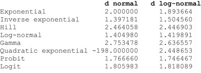
Non‐linear models
Non‐linear models need more attention during the implementation and estimation process, as compared to linear models. Non‐linear model components typically complicate identifiability, reduce precision of parameter estimation and lead to delayed convergence in iterative frequentist estimation procedures and Bayesian MCMC sampling. Estimates of non‐linear parameters may be highly correlated with each other, hindering simultaneous estimation of the parameters. It needs careful selection of starting values and it might be required to use particular constraints in the frequentist setting and (weakly) informative priors to stabilise the estimation process in a Bayesian application setting (see e.g. Chapter 10 in Congdon, 2006).
All 16 candidate models for the mean function in case of a continuous endpoint, and all 8 candidate models for the probability function are non‐linear models.
Appendix C – Data Examples: Continuous Endpoints
The appendix contains simulated examples based on the description in Section 2.6.3 to produce the generic Figures 3.1, 3.2 and 3.3 as well as the example analysed in the previous update of the guidance.
Example generated based on Figure 3.1
The Data
This example concerns a simulated data set, generated as a log‐normal exponential models with parameters a = 2.015, b = 1.5, c = 1.344 and d = 1.8, with dose levels 0,0.5,1,2,3 and a constant group size of 20. With a BMR = 0.10, the true BMD equals 0.2287.

The Bartlett test did reject the assumption of constant variance (normal distribution) with a p‐value of 0.00; and did not reject the assumption of constant coefficient of variation (lognormal distribution), with p‐values 0.46. These findings are to be expected as the data are generated according to the log‐normal distribution.
Results
PROAST. The EFSA BMD WEB app (https://doi.org/10.5281/zenodo.3760370) produce the following results of BMD modelling, using the exponential, inverse exponential, Hill and lognormal model, considering model averaging based on 1,000 bootstraps, by means of PROAST 70.0. The BMR was selected at 10%. For the exponential model the BMD was estimated as 0.184 with BMDL = 0.149 and BMDU = 0.220; for the inverse exponential model the BMD estimate was 0.103 with BMDL = 0.085 and BMDU = 0.121; for the Hill model the BMD estimate was 0.241 with BMDL = 0.203 and BMDU = 0.277; and for the lognormal model the BMD estimate was 0.171 with BMDL = 0.156 and BMDU = 0.185. The model averaging results produced BMDL = 0.172 and BMDU = 0.253. The ratio , indicating the precision of the estimation of the BMD.
Using Laplace approximation. First of all, the Bayes factor comparing the best model with the saturated model equals 9.41, indicating limited evidence against the best fitting model and consequently we can assume at least one candidate model fits reasonably well to the data.
The model‐specific results (BMDL, BMD, BMDU, weight) are given in Table C.1. This table shows that (i) the model‐specific BMDL's vary from 0.12 to 0.30, (ii) all normal models get weight close to 0.0000 (as to be expected), (iii) the weights for the log‐normal models vary from 0.08 to 0.23, with the highest weight 0.23 for the gamma model, and weight 0.096 for the true exponential model, and (iv) the model‐specific CrI's do differ substantially; some of them are even not overlapping.
Table C.1.
The 3.1 Example. Model‐specific values for BMDL, BMD and BMDU; and the posterior weights of each model (used for constructing the model average)

|
More information for the log‐normal gamma model is depicted in Figure C.1, with, for the background and minimum median response, and the BMD, the flat uninformative PERT prior distributions (in blue) and the final posterior distributions (in orange). The fourth parameter d (left lower panel) gets a log‐normal prior distribution (in blue), which is moderately informative with median at exp(1) = 2.72, in order to stabilise the fitting computationally. Similar plots can be made for all other 15 models.
Figure C.1.

The 3.1 Example: prior and posterior densities (pink and orange coloured respectively) for the background response, the maximum response, the BMD, and the parameter d, for the normal‐quadratic exponential model. The vertical dashed lines in the upper panels are the observed values for the background and maximum response
Using the weights of Table C.1 (last column), the final model‐averaged BMD estimate equals 0.245, close to the true value of 0.2349, with 90% CrI (0.1572, 0.3329), similar to the results obtained using the EFSA BMD WEB App. Based on the Laplace approximation results, the ratio is slightly larger (2.1), the estimation of the BMD is slightly more uncertain. Figure C.2 shows, on the log‐scale, the summary data together with the model‐specific fitted dose–response models, together with the CrI (in green), the BMD estimate (red bullet point), and the posterior distribution of the BMD, with the 90% CrI (in green) and the BMD estimate (red bullet point). Note how the fitted models vary substantially in the range from dose 0 to the first dose level; also, the posterior density of the BMD (in the lower right panel) shows some different peaks coming from mixing quite different posterior densities of the individual models (see also the quite different CrI's in Table C.1).
Figure C.2.

The 3.1 Example: based on the Laplace approximation: fitted normal dose–response models (upper left), fitted log‐normal dose–response models (upper right), all fitted models (lower left), averaged model with posterior density of the BMD, with 90% credible interval (in green) and BMD point estimate (in red)
Using MCMC. Using MCMC (hybrid and Bridge sampling), the results are quite similar. The final model‐averaged BMD estimate, obtained with Bridge sampling, equals 0.247 with 90% CrI (0.1640, 0.3380). The estimates for the hybrid method are 0.234 for the point estimate, and (0.1571, 0.3315) for the credible interval.
Results using individual data instead of summary data
As the data are simulated, the individual data are available as well. In this section, we illustrate how individual data can be further tested for distributional assumptions and how the use of summary data versus individual data affects the results of the analysis. The individual data are shown in Figure C.3.
Figure C.3.

The 3.1 Example: individual data with the summary arithmetic means (in red)
Distributional assumptions
Based on the summary data, the Bartlett test did reject the assumption of constant variance (normal distribution) and did not reject the assumption of constant coefficient of variation (log‐normal distribution) at the level of 5%. These findings are to be expected as the data are generated according to the log‐normal distribution. The Bartlett test focuses on the spread in the distribution and how it changes or not across the dose range. With the Shapiro–Wilk test, the normality and log‐normality assumption can be tested in more detail, at each dose level separately or across doses using the residuals of an ANOVA model. The test at each dose level separately looks most genuinely into the distributional model assumptions, but typically only based on a small sample size (20 in this case) and therefore might lack power. The global test on the ANOVA residuals is more powerful, as the sample size is much larger, but it assumes the distribution of the response data does not change across dose (except for the central location), such that centred residuals can be pooled.
The results in Table C.2 show that there is little evidence against normality, and against log‐normality. We do not expect to detect evidence against log‐normality, but we might have hoped to find evidence against normality. Locally, there seems to only be some limited evidence at the highest dose level, but some slight evidence also holds against the log‐normal distribution for that highest dose. Limited power is very likely an issue. Figure C.3 does not show very skewed (to the right) scatters of the data.
Table C.2.
The 3.1 Example. Results of Shapiro's test for normality and log‐normality (normality on log scale), at each dose level separately and globally, across all dose levels

|
The Bartlett test and the Shapiro–Wilk test complement each other quite well in checking distributional assumptions. Whereas the Bartlett test focuses on the pattern of the dispersion, the spread of the distribution, across the dose levels, the Shapiro–Wilk test focuses on how the location of the individual data is in line with the expected location but has little power when applied locally at each dose level because of too limited sample size. For this data set, the Bartlett test is able to lead us to the right conclusion.
How does approximating the geometric summary data affect the analysis?
The geometric mean and standard deviation (on the original scale) approximated from the arithmetic mean and standard deviation, as well as the exact geometric mean and standard deviation (directly computed from the individual data) are shown in Table C.3. For this particular data set, the approximation works very well, such that the differences are negligible, and the final BMD estimates are almost identical. Using the individual data and the exact geometric summary data, the model‐averaged BMD (using the Laplace approximation) equals 0.2351 with BMDL = 0.1564 and BMDU = 0.3325, very close to those based on the approximate geometric means and standard deviations.
Table C.3.
The 3.1 Example. Geometric means and standard deviationsapproximately using the arithmetic versions, in the first two columns; exactly as computed from the individual data in the last two columns

|
Example generated based on Figure 3.2
The Data
This example concerns a simulated data set, generated as a log‐normal exponential models with parameters a = 2.015, b = 1.5, c = 1.344 and d = 1.8, with dose levels 0,3,6,8,10 and a constant group size of 20. With a BMR = 0.10, the true BMD equals 0.2287.

The Bartlett test did reject the assumption of constant variance (normal distribution) with a p‐value of 0.00; and did not reject the assumption of constant coefficient of variation (lognormal distribution), with p‐values 0.46. These findings are to be expected as the data are generated according to the log‐normal distribution.
Results
PROAST. The EFSA BMD WEB app produce the following results of BMD modelling, using the exponential, inverse exponential, Hill and lognormal model, considering model averaging based on 1,000 bootstraps, by means of PROAST 70.0. The BMR was selected at 10%. For the exponential model the BMD was estimated as 0.04, not providing confidence limits; for the inverse exponential model the BMD estimate was 0.000001, not providing confidence limits; for the Hill model the BMD estimate was 0.000001, not providing confidence limits and for the lognormal model the BMD estimate was 0.002, not providing confidence limits. The model averaging results produced BMDL = 0.000001 and BMDU = 0.018. The ratio , indicating the uncertainty range of the estimation of the BMD.
Using Laplace approximation. The Bayes factor comparing the best model with the saturated model equals 5.86, indicating limited evidence against the best fitting model, and consequently we can assume at least one candidate model fits reasonably well to the data.
Not unexpectedly, as the response at the first active dose is already at its maximum and consequently the data contain no information about the dose–response pattern from the background to the maximum response, the individual model and the model‐averaged intervals are very wide and the BMDL are all essentially equal to or very close to 0. In addition, the estimation procedure leads to an infinite value of the BMDU. As the MCMC results are more precise and useful, we report more details about this approach.
Using MCMC. The Bayes factor BF = 6.33, indicating at least one candidate model fits reasonably well to the data. All models except for the (gamma, normal) model converged. The model‐specific results (BML, BMD, BMDU, weight) are given in Table C.4, showing quite a large difference between the Laplace and the MCMC based weights (see last two columns), indicating instability and/or inappropriateness of the Laplace approximation. This table shows that (i) the model‐specific BMDL's vary from 0.006 to 0.06, (ii) all normal models get weight close to 0.0000 (as to be expected as the data are log‐normal), (iii) the weights for the log‐normal models vary from 0.001 to 0.56, with the highest weight 0.56 for the probit model, followed by the logit model (weight 0.24). The true exponential model gets a low weight 0.02, and (iv) the model‐specific CrI's do differ substantially and are quite wide. In general, there is an overestimation of the true BMD = 0.229 (model‐specific point estimates tend to be larger than this true value).
Table C.4.
The 3.2 Example. Model‐specific values for BMDL, BMD and BMDU; and the posterior weights of each model (used for constructing the model average)

|
More information for the (probit, log‐normal) model is depicted in Figure C.4, with, for the background and maximum median response, and the BMD, the un−/weakly informative PERT prior distributions (in blue) and the final posterior distributions (in orange). The fourth parameter d (left lower panel) gets a log‐normal prior distribution (in blue), which is moderately informative with median at exp(1) = 2.72, in order to stabilise the fitting computationally. Similar plots can be made for all other 15 models.
Figure C.4.

The 3.2 Example: prior and posterior densities (pink and orange coloured respectively) for the background response, the maximum response, the BMD, and the parameter d, for the normal‐quadratic exponential model. The vertical dashed lines in the upper panels are the observed values for the background and maximum response
Using the weights of Table C.2 (last column) and based on Bridge sampling, the final model‐averaged BMD estimate equals 0.597, larger than the true value of 0.229, with 90% CrI (0.041, 1.887). The ratio of is equal to 14.6 and for is around 46, indicating uncertainty in the estimation of the BMD, but it is already improved in comparison to the results obtained when using the frequentist approach (PROAST). Note that the BMDL is about 6 times smaller than the true BMD and that the CrI covers slightly more than half of the range (0,3) (3 being the first active dose). Figure C.5 shows, on the log‐scale, the summary data together with the model‐specific fitted dose–response models, together with the CrI (in green), the BMD estimate (red bullet point), and the posterior distribution of the BMD, with the 90% CrI (in green) and the BMD estimate (red bullet point). Note how the fitted models vary substantially in the range from dose 0 to the first dose level, resulting in very different BMD estimates. As no data are available in the range (0,3) (covering the range 0 to more than 10 times the true BMD), no model can be informed by such data, and the different models adapt optimally to the available data on the higher dose levels, with the consequence that the fits deviate a lot in the dose range of interest.
Figure C.5.

The 3.2 Example: based on the Bridge sampling: fitted normal dose–response models (upper left), fitted log‐normal dose–response models (upper right), all fitted models (lower left), averaged model with posterior density of the BMD, with 90% credible interval (in green) and BMD point estimate (in red)
Using informative priors. We fit the same data again but with different informative priors on the BMD. Remember that the true value of the BMD = 0.229. The table below shows the impact of using informative priors in comparison to uninformative ones. When no mode is used to inform the prior distribution of the BMD, the estimation procedures does not improve the precision in estimation, being very large if Laplace approximation is used and around 50 when Bridge sampling is used. It is clear that if the range in which the BMD should be located is restricted and a most likely value is provided, the estimation precision improves drastically with a ratio for Laplace approximation smaller than 12 for Laplace and less than 8 for Bridge sampling. It is also worth noting that if the informative prior is misspecified, then the resulting BMD estimation might be as well biased.
We observe that (Table C.5), for this data set:
The Laplace approximation acts poorly unless the BMD priors is informative enough.
Bridge sampling outperforms the Laplace approximation, especially for less informative priors.
The Bridge CrI's are narrower than the Laplace CrI's.
An informative prior affects the BMDU more than the BMDL (reflecting the gain in accuracy).
Flat informative priors have less effect than focused priors on the same range (as expected).
A very informative incorrect prior affects the BMD estimation and biases the results.
Table C.5.
The 3.2 Example. BMD estimates for different choices of priors for the BMD parameter
| Informative prior on BMD |
Laplace approximation BMD and CrI |
Bridge sampling BMD and CrI |
|---|---|---|
| Uninformative prior | (0.000, Inf) | 0.597 (0.041, 1.887) |
| Uniform PERT prior on (0,3) | 0.100 (0.000, Inf) | 0.601 (0.042, 2.085) |
| PERT prior on (0,3) with mode 1 | 0.813 (0.215, 2.498) | 0.812 (0.218, 1.716) |
| Uniform PERT prior on (0,1) | 0.121 (0.000, Inf) | 0.389 (0.029, 0.924) |
| PERT prior on (0,1) with mode 0.5 | 0.480 (0.196, 1.107) | 0.467 (0.165, 0.785) |
| Uniform PERT prior on (0,0.5) | 0.015 (0.000, Inf) | 0.213 (0.019, 0.467) |
| PERT prior on (0,0.5) with mode 0.2 | 0.191 (0.069, 0.539) | 0.198 (0.059, 0.368) |
| PERT prior on (0.199,0.259) with mode 0.229 | 0.229 (0.206, 0.255) | 0.229 (0.210, 0.248) |
| PERT prior on (0.109,0.169) with mode 0.139 | 0.139 (0.116, 0.166) | 0.139 (0.120, 0.158) |
When using informative prior, is important to base its definition on data that can be verifiable and if very informative priors are used (see the two last rows of the table), the posterior is fully determined by the prior distribution. This could produce biased results in case that misspecified priors are used (see last row of the table).
Example generated based on Figure 3.3
The Data
This example concerns a simulated data set, generated as a log‐normal exponential models with parameters a = 2.015, b = 1.5, c = 1.344 and d = 1.8, with dose levels 0, 0.025, 0.05, 0.15, 0.4 and a constant group size of 20. With a BMR = 0.10, the true BMD equals 0.2287.

The Bartlett test did not reject the assumption of constant variance (normal distribution) with a p‐value of 0.25; and did not reject the assumption of constant coefficient of variation (lognormal distribution), with p‐values 0.46.
Results
PROAST. The EFSA BMD WEB app produce the following results of BMD modelling, using the exponential, inverse exponential, Hill and lognormal model, considering model averaging based on 1,000 bootstraps, by means of PROAST 70.0. The BMR was selected at 10%. For the exponential model the BMD was estimated as 0.226 with BMDL = 0.18 and BMDU = 0.275; for the inverse exponential model the BMD estimate was 0.223 with BMDL = 0.182 and BMDU = 0.265; for the Hill model the BMD estimate was 0.226 with BMDL = 0.18 and BMDU = 0.275 and for the lognormal model the BMD estimate was 0.225 with BMDL = 0.181 and BMDU = 0.269. The model averaging results produced BMDL = 0.175 and BMDU = 0.272. The ratio , indicating the precision of the estimation of the BMD.
Using Laplace approximation. The Bayes factor comparing the best model with the saturated model equals 4.82, indicating limited evidence against the best fitting model, and consequently we can assume at least one candidate model fits reasonably well to the data.
The model‐specific results (BML, BMD, BMDU, weight) are given in Table C.6, showing that (i) the model‐specific BMDL's vary from 0.172 to 0.290, (ii) the weights vary across all 16 models, but with higher weights for the log‐normal models iii) the highest weight is for the (quadratic exponential, log‐normal) model (0.21) and weights vary from 0.04 to 0.12 for all other log‐normal models. The normal models have weights about 0.001 to 0.06.
Table C.6.
The 3.3 Example. Model‐specific values for BMDL, BMD and BMDU; and the posterior weights of each model (used for constructing the model average)

|
More information for the log‐normal quadratic exponential model is depicted in Figure C.6, with, for the background and maximum median response, and the BMD, the un−/weakly informative PERT prior distributions (in blue) and the final posterior distributions (in orange). For this particular example, since the highest experimental dose is smaller than 1 (i.e. 0.4), the PERT prior for the BMD is set as approximately uniform on the interval [0, 400]. For clarity, the range in the plot is set to the interval [0, 0.4], resulting in a seemingly peaked prior due to some variability in the simulated prior values. The fourth parameter d (left lower panel) gets a log‐normal prior distribution (in blue), which is moderately informative with median at exp(1) = 2.72, in order to stabilise the fitting computationally. Similar plots can be made for all other 15 models.
Figure C.6.

The 3.3 Example: prior and posterior densities (pink and orange coloured respectively) for the background response, the maximum response, the BMD and the parameter d, for the normal‐quadratic exponential model. The vertical dashed lines in the upper panels are the observed values for the background and maximum response
Using the weights of Table C.6 (last column), the final model‐averaged BMD estimate equals 0.2202, quite close to the true value of 0.229, with 90% CrI (0.1818, 0.2701), similar to the results obtained using the EFSA BMD WEB App. Note that this CrI includes the true value 0.229. Based on the Laplace approximation results, the ratio is slightly smaller (1.48), the estimation of the BMD is slightly more precise. Figure C.7 shows, on the log‐scale, the summary data together with the model‐specific fitted dose–response models, together with the CrI (in green), the BMD estimate (red bullet point), and the posterior distribution of the BMD, with the 90% CrI (in green) and the BMD estimate (red bullet point). Note how the fitted models vary substantially in the range from dose 0 to the first dose level, resulting in very different BMD estimates.
Figure C.7.

The 3.3 Example: based on the Bridge sampling: fitted normal dose–response models (upper left), fitted log‐normal dose–response models (upper right), all fitted models (lower left), averaged model with posterior density of the BMD, with 90% credible interval (in green) and BMD point estimate (in red)
Using MCMC. Using MCMC (hybrid and Bridge sampling), the results are similar. The Bayes factor equals 5.40. The final model‐averaged BMD estimate, obtained with Bridge sampling, equals 0.2225 with 90% CrI (0.1786, 0.2763). The estimates for the hybrid method are 0.2216 for the point estimate, and (0.1781, 0.2750) for the credible interval.
The Body Weight Example in the 2017 EFSA Guidance Update
The Data
See Example 1 in Section 2.5.9 of EFSA SC (2017). The data in this example relate to a 2‐year study in male mice. A dose‐related decrease in body weight was observed. This endpoint is assumed to be the critical effect and the BMR considered is 5%.
| Dose (mg /kg bw per day) | Body weight, group mean (g) | SD | n |
|---|---|---|---|
| 0 | 43.85 | 2.69 | 37 |
| 0.1 | 43.51 | 2.86 | 35 |
| 0.5 | 40.04 | 3 | 43 |
| 1.1 | 35.09 | 2.56 | 42 |
bw: body weight; SD: Standard deviation.
The Bartlett test did not reject the assumption of constant variance (normal distribution) nor the assumption of constant coefficient of variation (lognormal distribution), with p‐values 0.76 and 0.59 respectively.
Results
PROAST. Using PROAST v. 61.6 with the default BMR of 5% and applying the Exponential and the Hill model, the BMDL in EFSA SC (2017) was determined to be 0.20 mg/kg, with BMDU = 0.41 mg/kg. The EFSA BMD WEB app produce the following results of BMD modelling, using the exponential, inverse exponential, Hill and lognormal model, considering model averaging based on 1,000 bootstraps, by means of PROAST 70.0. The BMR was selected at 5%. For the exponential model the BMD was estimated as 0.297 with BMDL = 0.198 and BMDU = 0.41; for the inverse exponential model the BMD estimate was 0.316 with BMDL = 0.219 and BMDU = 0.422; for the Hill model the BMD estimate was 0.297 with BMDL = 0.198 and BMDU = 0.41 and for the lognormal model the BMD estimate was 0.308 with BMDL = 0.21 and BMDU = 0.416. The model averaging results produced BMDL = 0.216 and BMDU = 0.419. The ratio , indicating the precision of the estimation of the BMD.
Here, all 16 models are used, with equal prior probabilities 1/16 and with uninformative priors on the model parameters, again with BMR = 5%.
Using Laplace approximation. First of all, the Bayes factor comparing the best model with the saturated model equals 0.94, indicating the best fitting model and consequently at least one candidate model fits well to the data. The model‐specific results (BML, BMD, BMDU, weight) are given in Table C.7. The table shows that (i) the model‐specific BMDL's vary from 0.216 to 0.297, (ii) the highest weights are assigned to the quadratic exponential models, with weight 0.187 and 0.224 for the normal and log‐normal version respectively, (iii) weights are quite evenly distributed across the remaining models.
Table C.7.
The Body Weight Example in the 2017 EFSA Guidance Update. Model‐specific values for BMDL, BMD and BMDU; and the posterior weights of each model (used for constructing the model average)

|
More information for the log‐normal quadratic exponential model is depicted in Figure C.7 with uninformative PERT prior distributions (in blue) for the background and maximum median response (in this case a negative decreasing response), and a flat uninformative PERT prior distribution for (in blue) the BMD, and the final posterior distributions (in orange). Actually, the prior for the maximum response is weakly informative. The reason for that is that the maximum response is not reached at the end of the experimental dose range (see Figure C.8). The prior for the minimum response is therefore centred at half of the observed mean response at the highest dose (35.09/2 = 17.545), with a considerably large uncertainty range. As there is little or no information in the data about this minimum response, the posterior density remains close to the prior density (right upper panel of Figure C.7). Finally, for the fourth parameter d (left lower panel), the log‐normal prior distribution (in blue) is moderately informative with median at the value of exp(1) = 2.72, in order to stabilise the fitting computationally. The orange posterior distribution peaks around the median of the prior distribution, shifted somewhat to the right. Similar plots can be made for all other 15 models.
Figure C.7.

The Body Weight Example in the 2017 EFSA Guidance Update: prior and posterior densities (blue and orange coloured respectively) for the background response, the maximum response, the BMD and the parameter d, for the log‐normal quadratic exponential model. The vertical dashed lines in the upper panels are the observed values for the background and maximum response
Figure C.8.

The Body Weight Example in the 2017 EFSA Guidance Update: based on the Laplace approximation, model‐specific fitted dose–response models, together with the CrI (in green) and the BMD estimate (red bullet point). Upper left: normal models; upper right: log‐normal models; Lower left: all models; Lower right: model‐averaged fitted dose–response model, together with the posterior distribution of the BMD
Using the weights of Table C.4 (last column), the final model‐averaged BMD estimate equals 0.310 with 90% CrI (0.225,0.428). So, the BMDL = 0.225 mg/kg, with BMDU = 0.428 mg/kg, quite similar to the results in EFSA SC (2017) and the very similar if we would have analysed it using the EFSA WEB app.
Figure C.8 shows, on the log‐scale, the summary data together with the model‐specific fitted dose–response models, together with the CrI (in green) and the BMD estimate (red bullet point). The lower right panel shows the posterior density of the BMD.
Using MCMC. Using MCMC (hybrid and Bridge sampling), the results are very similar. The final model‐averaged BMD estimate, obtained with Bridge sampling, equals 0.318 with 90% CrI (0.227,0.430).
Appendix D – Data Examples: Quantal Endpoints
Thyroid epithelial cell vacuolisation data in the 2017 EFSA Guidance Update
The Data
This example relates to a 2‐year study in rats, where three doses of a substance were administered to the animals. Dose‐related changes in thyroid epithelial cell vacuolisation were found, and these data were used for a BMD analysis.
| Dose (mg/kg day) | No of animals with thyroid epithelial vacuolisation | No of animals in dose group |
|---|---|---|
| 0 | 6 | 50 |
| 3 | 6 | 50 |
| 12 | 34 | 50 |
| 30 | 42 | 50 |
Results
PROAST. Using PROAST v 62.3 together with the MADr‐BMD program, as described in Wheeler and Bailer (2008), using the default BMR of 10% extra risk, using all 8 models except the exponential model, and using the bootstrap, the BMDL in EFSA SC (2017) was determined to be 1.5 mg/kg (a BMDU was not calculated). Using the EFSA BMD WEB app (based on PROAST 70.0), the model‐averaged BMDL = 1.65 and BMDU = 5.86. The ratio , indicating the precision of the estimation of the BMD
Using Laplace approximation. The model‐specific results (BML, BMD, BMDU, weight) are given in Table D.1, showing that (i) the model‐specific BMDL's vary from 1.467 to 2.709, (ii) the weights vary substantially across all 8 models, (iii) the highest weight 0.40 is given to the inverse exponential model, followed by the Hill model with weight 0.17, and all other models with weights below 0.1 except for log‐normal and gamma models. The Bayes factor is 13.76 in favour of the inverse exponential model over the saturated model.
Table D.1.
The thyroid epithelial cell vacuolisation data. Model‐specific values for BMDL, BMD and BMDU; and the posterior weights of each model (used for constructing the model average)

|
More information for the inverse exponential model is depicted in Figure D.1, for the background and the BMD, the un−/weakly informative PERT prior distributions (in blue) and the final posterior distributions (in orange). The third parameter d (right upper panel) gets a log‐normal prior distribution (in blue) which is moderately informative with median at exp(1) = 2.72, in order to stabilise the fitting computationally. Similar plots can be made for all other 7 models.
Figure D.1.

The thyroid epithelial cell vacuolisation data: prior and posterior densities (pink and orange coloured respectively) for the background response, the BMD and the parameter d, for the inverse exponential model. The vertical dashed line in the upper right panel is the observed background proportion
Using the weights of Table D.1 (last column), the final model‐averaged BMD estimate equals 4.207 with 90% CrI (2.149, 8.314). These results are quite close to the PROAST results. Based on the Laplace approximation results, the ratio is slightly larger (3.87). Although it can be said that these results are quite close to the PROAST results. Figure D.2 shows, on the log‐scale, the summary data together with the model‐specific fitted dose–response models, together with the CrI (in green), the BMD estimate (red bullet point), and the posterior distribution of the BMD, with the 90% CrI (in green) and the BMD estimate (red bullet point). Note how the fitted models vary substantially close the first active dose level, resulting in quite different BMD estimates.
Figure D.2.

The thyroid epithelial cell vacuolisation data: based on Laplace: fitted normal dose–response models (left), averaged model with posterior density of the BMD, with 90% credible interval (in green) and BMD point estimate in red (right)
Using MCMC. The results are quite similar with the inverse exponential model receiving a similar weight (0.417) as that obtained from Laplace, implying the averaged version to be pulled somewhat in the direction of the model‐specific values for the inverse exponential. The model‐averaged BMD estimate is 4.682 with 90% CrI (2.184, 7.667), achieving a higher precision .
Appendix E – Template for reporting a BMD analysis
A Data description
Brief general description of the data. This section should include a table summarising the data. In case that raw data is available, resulting in a too large table, summary statistics may be given instead.12 For quantal endpoints both the number of responding animals and the total number of animals should be given for each dose level; for continuous endpoints either the individual responses or the mean responses and the associated SDs (or SEMs) and sample sizes should be given for each dose level.
Example of table for continuous dose–response data
| Dose | Endpoint mean | SD | N | Covariates (gender) |
|---|---|---|---|---|
| 0 | 43.85 | 2.69 | 37 | M |
| 0.1 | 43.51 | 2.86 | 35 | M |
| 0.5 | 40.04 | 3.00 | 43 | M |
| 1.1 | 35.09 | 2.56 | 42 | M |
| 0 | 41.54 | 6.26 | 36 | F |
| 0.1 | 38.71 | 4.73 | 42 | F |
| 0.5 | 33.76 | 3.92 | 37 | F |
| 1.1 | 28.55 | 2.08 | 38 | F |
In case that several control groups are reported in the publication or provided by the applicant, they should all be presented in the table. How these will be handled in the analysis needs a case‐by‐case consideration.
Example of table for quantal dose–response data
| Dose | Number of animals with event of interest | N | Covariates (gender) |
|---|---|---|---|
| 0 | 2 | 50 | M |
| 3 | 4 | 50 | M |
| 12 | 32 | 49 | M |
| 30 | 45 | 50 | M |
| 0 | 6 | 50 | F |
| 3 | 6 | 50 | F |
| 12 | 34 | 50 | F |
| 30 | 42 | 50 | F |
In case different endpoints are to be analysed, they should be described in different subsections, containing information pertaining to each endpoint.
The following steps apply for each endpoint considered.
B Selection of the BMR
The value of the BMR used in the analysis. The rationale behind the choice made (the biological relevance in the case of a continuous endpoint) should be described.
C Software used
The software used, including version number should be reported. In case another non‐publicly available software was used, the script for the BMD analysis should be provided as an appendix.
D Justification of any deviation from the procedure and assumptions
In case another approach than Bayesian model averaging was used, the rationale and details for deviating from the recommended approach should be provided.
Assumptions made when deviating from the recommended defaults in this guidance document (e.g. gamma distributional assumption instead of normal and log‐normal, heteroscedasticity instead of homoscedasticity).
Other models than the recommended ones listed in Tables 2 and 3 of this guidance document that were fitted should be listed, with the reasons to include them.
Description of any deviation from the procedure described in the flow chart (Figure 2) to obtain the final BMD credible interval.
E Results
The results of the BMD analysis should contain:
In case where individual data are available, the results of the distributional assumption test.
Results of the Bartlett test (see Section 2.5.1).
A table presenting the results of the models fitted, BMD, BMDL, BMDU and model weight (see Table below).
Report whenever convergence issues were encountered.
Report whether none of the candidate models fit sufficiently well to the data (see Section 2.5.3).
Result table for continuous/quantal data.
| Model | BMDL | BMD | BMDU | Model Weights |
|---|---|---|---|---|
| Exponential (E4) | ||||
| Inverse Exponential (IE4) | ||||
| Hill (H4) | ||||
| Log‐normal (LN4) | ||||
| Gamma (G4) | ||||
| Two‐Stage (QE4) | ||||
| Probit (P4) | ||||
| Logit (L4) |
F Plots of fitted models
Show the plot of the data with credible intervals for the responses, together with the resulting models as well as the model average fit (Figure E.1).
G Conclusions
This section should summarise the results for each endpoint (data set) that was analysed and provide a discussion of the rationale behind selecting the critical endpoint.
The BMD credible interval of the critical endpoint (and the BMDL selected as RP) should be reported and discussed.
Suggested citation: EFSA Scientific Committee , More SJ, Bampidis V, Benford D, Bragard C, Halldorsson TI, Hernández‐Jerez AF, Bennekou SH, Koutsoumanis K, Lambré C, Machera K, Mennes W, Mullins E, Nielsen SS, Schrenk D, Turck D, Younes M, Aerts M, Edler L, Sand S, Wright M, Binaglia M, Bottex B, Cortiñas Abrahantes J and Schlatter J, 2022. Guidance on the use of the benchmark dose approach in risk assessment. EFSA Journal 2022;20(10):7584, 67 pp. 10.2903/j.efsa.2022.7584
Requestor: EFSA
Question number: EFSA‐Q‐2020‐00137
Panel members: Simon John More, Vasileios Bampidis, Diane Benford, Claude Bragard, Thorhallur Ingi Halldorsson, Antonio F Hernández‐Jerez, Susanne Hougaard Bennekou, Kostas Koutsoumanis, Claude Lambré, Kyriaki Machera, Ewen Mullins, Søren Saxmose Nielsen, Josef Schlatter, Dieter Schrenk, Dominique Turck and Maged Younes.
Note: The outcome of the public consultation on this draft opinion with QN ‘EFSA‐Q‐2020‐00139’ should be published on the same day and should be cross‐referenced.An external technical report with QN ‘EFSA‐Q‐2019‐00417’ and ‘EFSA‐Q‐2020‐00138’ will be published and should be cross‐referenced.
Declarations of interest: If you wish to access the declaration of interests of any expert contributing to an EFSA scientific assessment, please contact interestmanagement@efsa.europa.eu.
Acknowledgements: The Scientific Committee wishes to thank Maria Chiara Astuto and Hans Steinkellner for the support provided to this scientific output.
Adopted: 21 September 2022
This publication is linked to the following EFSA Supporting Publications article: http://onlinelibrary.wiley.com/doi/10.2903/sp.efsa.2022.EN-7585/full
Notes
The outcome of the public consultation is published as a stand‐alone technical report (EFSA‐Q‐2020‐00139).
Following EFSA's reorganisation of 1 January 2022, this responsibility has been transferred to the Methodology & Scientific Support (MESE) Unit.
The term ‘confidence interval’ is used in the context of frequentist statistics while the term ‘credible interval’ is used in a Bayesian paradigm, see Section 2.5.3.
In this regard, two external technical reports will be published https://open.efsa.europa.eu/questions/EFSA‐Q‐2020‐00138?search=EFSA‐Q‐2020‐00138 and https://open.efsa.europa.eu/questions/EFSA‐Q‐2019‐00417?search=EFSA‐Q‐2019‐00417
In this opinion, ‘response’ is used as a generic term that refers to both quantal and continuous data.
The word ‘biologically relevant’ is preferred to ‘adverse’ to allow, e.g. for the use of the BMD approach with biomarkers of effect that are not necessarily adverse.
For any endpoint in a given test species, there is a true value for the BMD parameter, and any study provides information about this true value.
The total number of events is then binomially distributed.
If the BMD is lower than 10 times the lowest non‐zero dose, a possible alternative is using the N(L)OAEL see further down.
Note that, when the individual data were used in the original analysis, slightly different results may be obtained using the summary data in the analysis.
References
- Aerts M, Molenberghs G, Ryan LM and Geys H, 2002. Topics in Modelling of Clustered Data. 1st edn. Chapman and Hall/CRC. 10.1201/9781420035889 [DOI] [Google Scholar]
- Aerts M, Wheeler MW and Cortinas Abrahantes J, 2020. An extended and unified modelling framework for benchmark dose estimation for both continuous and binary data. Environmetrics, 31, e2630. 10.1002/env.2630 [DOI] [PMC free article] [PubMed] [Google Scholar]
- Allen BC, Kavlock RJ, Kimmel CA and Faustman EM, 1994. Dose‐response assessment for developmental toxicity. II. Comparison of generic Benchmark dose estimates with No Observed Adverse Effects Levels. Fundamental and Applied Toxicology, 23, 487–495. [DOI] [PubMed] [Google Scholar]
- Bartlett MS, 1937. Properties of sufficiency and statistical tests. Proceedings of the Royal Statistical Society, Series A, 160, 268–282. [Google Scholar]
- Bayarri MJ and Berger JO, 2004. The Interplay of Bayesian and Frequentist Analysis. Statistical Science, 19, 58–80. [Google Scholar]
- Beausoleil C, Beronius A, Bodin L, Bokkers BGH, Boon PE, Burger M, Cao Y, De Wit L, Fischer A, Hanberg A, Leander K, Litens‐Karlsson S, Rousselle C, Slob W, Varret C, Wolterink G and Zilliacus J, 2016. Review of non‐monotonic dose‐responses of substances for human risk assessment. EFSA Supporting Publications 2016;13:1027E. 10.2903/sp.efsa.2016.EN-1027 [DOI] [Google Scholar]
- Bolstad WM and Curran JM, 2016. Introduction to Bayesian Statistics, John Wiley & Sons, Incorporated, 2016. ProQuest Ebook Central. Available online: https://ebookcentral.proquest.com/lib/ubhasselt/detail.action?docID=4658580 [Google Scholar]
- Bosgra S, van der Voet H, Boon PE and Slob W, 2009. An integrated probabilistic framework for cumulative risk assessment of common mechanism chemicals in food: an example with organophosphorus pesticides. Regulatory Toxicology and Pharmacology Journal, 54, 124–133. [DOI] [PubMed] [Google Scholar]
- Brown MB and Forsythe AB, 1974. Robust tests for the equality of variances. Journal of the American Statistical Association, 69, 364–367. 10.2307/2285659 [DOI] [Google Scholar]
- Burnham KP and Anderson DR, 2002. Model Selection and Multimodel Inference: A Practical Information‐Theoretical. Approach. 2d edn. Springer‐Verlag, New York. [Google Scholar]
- Burnham KP and Anderson DR, 2004. Multimodel Inference: Understanding AIC and BIC in Model Selection. Sociological Methods & Research, 33, 261–304. [Google Scholar]
- Congdon P, 2006. Bayesian Statistical Modelling. 2a. edn. Wiley, Chichester. [Google Scholar]
- Cox DR, 2006. Frequentist and Bayesian Statistics: A Critique. Transactions in Particle Physics, Astrophysics and Cosmology. [Google Scholar]
- Davis JA, Gift JS and Zhao QJ, 2011. Introduction to benchmark dose methods and U.S. EPA's benchmark dose software (BMDS) version 2.1.1. Toxicology and Applied Pharmacology, 254, 181–191. 10.1016/j.taap.2010.10.016 [DOI] [PubMed] [Google Scholar]
- Dekkers S, de Heer C and Rennen M, 2001. Critical effect sizes in toxicological risk assessment: a comprehensive and critical evaluation. Environmental Toxicology and Pharmacology, 10(1–2), 33–52. [DOI] [PubMed] [Google Scholar]
- EFSA (European Food Safety Authority) , 2004a. Opinion of the Scientific Panel on contaminants in the food chain [CONTAM] to assess the health risks to consumers associated with exposure to organotins in foodstuffs, EFSA Journal 2004;2(10):102, 119 pp. 10.2903/j.efsa.2004.102 [DOI] [Google Scholar]
- EFSA (European Food Safety Authority) , 2004b. Opinion of the Scientific Panel on contaminants in the food chain [CONTAM] related to Deoxynivalenol (DON) as undesirable substance in animal feed. EFSA Journal 2004;2(6):73, 42 pp. 10.2903/j.efsa.2004.73 [DOI] [Google Scholar]
- EFSA (European Food Safety Authority) , 2005a. Opinion of the Scientific Committee on a request from EFSA related to A Harmonised Approach for Risk Assessment of Substances Which are both Genotoxic and Carcinogenic. EFSA Journal 2005;3(10):282, 33 pp. 10.2903/j.efsa.2005.282 [DOI] [Google Scholar]
- EFSA (European Food Safety Authority) , 2005b. Opinion of the Scientific Panel on contaminants in the food chain [CONTAM] related to fumonisins as undesirable substances in animal feed. EFSA Journal 2005;3(7):235, 32 pp. 10.2903/j.efsa.2005.235 [DOI] [Google Scholar]
- EFSA (European Food Safety Authority) , 2007. Opinion of the Scientific Panel on food additives, flavourings, processing aids and materials in contact with food (AFC) related to an application on the use of ethyl lauroyl arginate as a food additive. EFSA Journal 2007;5(7):511, 27 pp. 10.2903/j.efsa.2007.511 [DOI] [Google Scholar]
- EFSA (European Food Safety Authority) , 2009. Guidance of the Scientific Committee on a request from EFSA on the use of the benchmark dose approach in risk assessment. EFSA Journal 2009;1150:1–72, 72 pp. 10.2903/j.efsa.2009.1150 [DOI] [Google Scholar]
- EFSA CONTAM Panel (EFSA Panel on Contaminants in the Food Chain) , 2011. Scientific Opinion on Pyrrolizidine alkaloids in food and feed. EFSA Journal 2011;9(11):2406, 134 pp. 10.2903/j.efsa.2011.2406. [DOI] [Google Scholar]
- EFSA (European Food Safety Authority) , 2014. Guidance on Expert Knowledge Elicitation in Food and Feed Safety Risk Assessment. EFSA Journal 2014;12(6):3734, 278 pp. 10.2903/j.efsa.2014.3734 [DOI] [Google Scholar]
- EFSA (European Food Safety Authority) , 2015. Tools for critically appraising different study designs, systematic review and literature searches. EFSA supporting publication 2015:EN‐836, 65 pp. 10.2903/sp.efsa.2015.EN-836 [DOI] [Google Scholar]
- EFSA Scientific Committee , 2015. Scientific Opinion: Guidance on the review, revision and development of EFSA's Cross‐cutting Guidance Documents. EFSA Journal 2015;13(4):4080, 11 pp. 10.2903/j.efsa.2015.4080 [DOI] [Google Scholar]
- EFSA Scientific Committee , Hardy, A , Benford, D , Halldorsson, T , Jeger, MJ , Knutsen, KH , More, S , Mortensen, A , Naegeli, H , Noteborn, H , Ockleford, C , Ricci, A , Rychen, G , Silano, V , Solecki, R , Turck, D , Aerts, M , Bodin, L , Davis, A , Edler, L , Gundert‐Remy, U , Sand, S , Slob, W , Bottex, B , Cortinas Abrahantes, J , Marques, DC , Kass, G and Schlatter, JR , 2017. Update: Guidance on the use of the benchmark dose approach in risk assessment. EFSA Journal 2017;15(1):4658, 41 pp. 10.2903/j.efsa.2017.4658 [DOI] [PMC free article] [PubMed] [Google Scholar]
- EFSA Scientific Committee , Benford D, Halldorsson T, Jeger MJ, Knutsen HK, More S, Naegeli H, Noteborn H, Ockleford C, Ricci A, Rychen G, Schlatter JR, Silano V, Solecki R, Turck D, Younes M, Craig P, Hart A, Von Goetz N, Koutsoumanis K, Mortensen A, Ossendorp B, Martino L, Merten C, Mosbach‐Schulz Oand Hardy A, 2018. Guidance on Uncertainty Analysis in Scientific Assessments. EFSA Journal 2018;16(1):5123, 39 pp. 10.2903/j.efsa.2018.5123 [DOI] [PMC free article] [PubMed] [Google Scholar]
- Fisher RA, 1922. On the mathematical foundations of theoretical statistics. Philosophical Transactions of the Royal Society A, 222, 309–368. [Google Scholar]
- Fowles JR, Alexeeff GV and Dodge D, 1999. The use of benchmark dose methodology with acute inhalation lethality data. Regulatory Toxicology and Pharmacology, 29, 262–278. [DOI] [PubMed] [Google Scholar]
- Haber LT, Dourson ML, Allen BC, Hertzberg RC, Parker A, Vincent MJ, Maier A and Boobis AR, 2018. Benchmark dose (BMD) modeling: current practice, issues, and challenges. Critical Reviews in Toxicology, 48, 387–415. 10.1080/10408444.2018.1430121 [DOI] [PubMed] [Google Scholar]
- Hoeting JA, Madigan D, Raftery AE and Volinsky CT, 1999. Bayesian model averaging: a tutorial. Statistical Science, 14, 382–417. [Google Scholar]
- Joint FAO/WHO Meeting on Pesticide Residues (JMPR) , 2000. Pesticide residues in food 2000, Toxicological evaluations, Thiodicarb. First draft prepared by I. Dewhurst Pesticides Safety Directorate, Ministry of Agriculture, Fisheries and Food, Mallard House, Kings Pool, York, United Kingdom. Available online: www.inchem.org/documents/jmpr/jmpmono/v00pr09.htm
- Joint FAO/WHO Meeting on Pesticide Residues (JMPR) , 2001a. Pesticide residues in food 2001, Toxicological evaluations, Carbaryl (addendum). First draft prepared by. In: van Apeldoorn ME, Wolterink G, Turkstra E, van Raaij MTM, van Hoeven‐Arentzen PH and van Engelen JGM (eds.). Centre For Substances and Risk Assessment. National Institute of Public Health and the Environment, Bilthoven, The Netherlands: Available online: www.inchem.org/documents/jmpr/jmpmono/2001pr02.htm [Google Scholar]
- Joint FAO/WHO Meeting on Pesticide Residues (JMPR) , 2001b. Pesticide residues in food 2001, Toxicological evaluations, Spinosad. First draft prepared by A. Bartholomaeus, Chemicals and Non‐prescription Medicines Branch, Therapeutic Goods Administration, Canberra ACT, Australia. Available online: www.inchem.org/documents/jmpr/jmpmono/2001pr12.htm
- Joint FAO/WHO Meeting on Pesticide Residues (JMPR) , 2002a. Pesticide residues in food 2002, Toxicological evaluations, Flutolanil. First draft prepared by I. Dewhurst, Pesticides Safety Directorate, Department for Environment, Food and Rural Affairs, Kings Pool, York, England. Available online: www.inchem.org/documents/jmpr/jmpmono/2002pr07.htm
- Joint FAO/WHO Meeting on Pesticide Residues (JMPR) , 2002b. Pesticide residues in food 2002, Toxicological evaluations, Metalaxyl and Metalaxyl‐M. First draft prepared by C. Vleminckx, Scientific Institute of Public Health, Division Toxicology, Brussels, Belgium. Available online: www.inchem.org/documents/jmpr/jmpmono/2002pr09.htm
- Joint FAO/WHO Meeting on Pesticide Residues (JMPR) , 2003a. Pesticide residues in food 2003, Toxicological evaluations, Cyprodinil. First draft prepared by P. V. Shah, United States Environmental Protection Agency, Office of Pesticide Programs, Washington DC, USA. Available online: www.inchem.org/documents/jmpr/jmpmono/v2003pr03.htm
- Joint FAO/WHO Meeting on Pesticide Residues (JMPR) , 2003b. Pesticide residues in food 2003, Toxicological evaluations, Famoxadone. First draft prepared by D.B. McGregor, Toxicology Evaluation Consultants, Lyon, France. Available online: www.inchem.org/documents/jmpr/jmpmono/v2003pr05.htm
- Joint FAO (Food and Agriculture Organization of the United Nations) and WHO (World Health Organization) Expert Committee on Food Additives (JECFA) , 2006a. Sixty‐fourth meeting, WHO/IPCS Safety evaluation of certain contaminants in food. WHO Food Additives Series 55. [PubMed]
- Johnson NL, Kotz S and Balakrishnan N, 1994. Continuous Univariate Distributions, Vol. 1. 2nd edn. John Wiley & Sons Ltd., New York. [Google Scholar]
- Johnson NL, Kotz S and Balakrishnan N, 1995. Continuous Univariate Distributions, Vol. 2. 2nd edn Section 25.4. edn. John Wiley & Sons Ltd., New York. [Google Scholar]
- Kruschke J, 2014. Doing Bayesian Data Analysis: A Tutorial with R, JAGS and Stan. Elsevier Science & Technology. ProQuest Ebook Central, https://ebookcentral.proquest.com/lib/ubhasselt/detail.action?docID=5754481
- Lehmann EL and Casella G, 1998. Theory of Point Estimation. 2nd edn. Springer. [Google Scholar]
- Lesaffre E and Lawson AB, 2012. Bayesian Biostatistics. John Wiley & Sons Ltd., New York. 534 p. ISBN 978–0–470‐01823‐1. [Google Scholar]
- Levene H, 1960. Robust tests for equality of variances. In: Olkin I (ed). Contributions to probability and statistics; essays in honor of Harold Hotelling. Stanford University Press, Stanford, Calif. [Google Scholar]
- Milton B, Krewski D, Mattison DR, Karyakina NA, Ramoju S, Shilnikova N, Birkett N, Farrell PJ and McGough D, 2017. Modeling U‐shaped dose‐response curves for manganese using categorical regression. Neurotoxicology, 58, 217–225. 10.1016/j.neuro.2016.10.001 [DOI] [PubMed] [Google Scholar]
- Morales KH, Ibrahim JG, Chen C‐J and Ryan LM, 2006. Bayesian model averaging with applications to benchmark dose estimation for arsenic in drinking water. Journal of the American Statistical Association, 101(473), 9–17. 10.1198/016214505000000961 [DOI] [Google Scholar]
- Sand S, Portier CJ and Krewski D, 2011. A Signal‐to‐Noise Crossover Dose as the Point of Departure for Health Risk Assessment. Environmental Health Perspectives, 119, 1766–1774. [DOI] [PMC free article] [PubMed] [Google Scholar]
- Sand S, 2021. A novel method for combining outcomes with different severities or gene‐level classifications. ALTEX ‐ Alternatives to Animal Experimentation, 39, 480–497. 10.14573/altex.2004212 [DOI] [PubMed] [Google Scholar]
- Shapiro SS and Wilk MB, 1965. An analysis of variance test for normality (complete samples). Biometrika, 52(3–4), 591–611. [Google Scholar]
- Slob W, 2002. Dose‐response modelling of continuous endpoints. Toxicological Sciences, 66, 298–312. [DOI] [PubMed] [Google Scholar]
- Slob W and Setzer RW, 2014. Shape and steepness of toxicological dose‐response relationships of continuous endpoints. Critical Reviews in Toxicology, 44, 270–297. [DOI] [PubMed] [Google Scholar]
- Slob W, 2017. A general theory of effect size, and its consequences for defining the benchmark response (BMR) for continuous endpoints. Critical Reviews in Toxicology, 47(4), 342–351. 10.1080/10408444.2016.1241756 [DOI] [PubMed] [Google Scholar]
- Stigler S, 1973. Studies in the History of Probability and Statistics. XXXII: Laplace, Fisher and the Discovery of the Concept of Sufficiency. Biometrika, 60(3), 439–445. [Google Scholar]
- Stoica P, Selén Y and Li J, 2004. Multi‐model approach to model selection. Digital Signal Processing, 14(5), 399–412. [Google Scholar]
- Teunis PFM, Evers EG and Slob W, 1999. Analysis of variable fractions resulting from microbial counts. Quantitative Microbiology, 1, 63–88. [Google Scholar]
- United States Environmental Protection Agency (US EPA) , 2012. Benchmark Dose Technical Guidance. (EPA/100/R‐12/001). Washington DC: Risk Assessment Forum. Available online: http://www.epa.gov/raf/publications/pdfs/benchmark_dose_guidance.pdf
- United States Environmental Protection Agency (US EPA) , 2016. Categorical Regression (CatReg) User Guide (Version 3.0.1.5). Available online: https://www.epa.gov/sites/production/files/2016-03/documents/catreg_user_guide.pdf
- United States Environmental Protection Agency (US EPA) , 2020. Benchmark Dose Software (BMDS) Version 3.2, User Guide. EPA/600/R‐20/216.
- Wignall JA, Shapiro AJ, Wright FA, Woodruff TJ, Chiu WA, Guyton KZ and Rusyn I, 2014. Standardizing benchmark dose calculations to improve science‐based decisions in human health assessments. Environmental Health Perspectives, 122, 499–505. 10.1289/ehp.1307539 [DOI] [PMC free article] [PubMed] [Google Scholar]
- Wheeler MW and Bailer AJ, 2008. Model averaging software for dichotomous dose response risk estimation. Journal of Statistical Software, 26, 1–15.19777145 [Google Scholar]
- Wheeler MW, Cortiñas Abrahantes J, Aerts M, Gift JS and Allen Davis J, 2022. Continuous model averaging for benchmark dose analysis: Averaging over distributional forms. Environmetrics, 33, e2728. 10.1002/env.2728 [DOI] [PMC free article] [PubMed] [Google Scholar]
- WHO (World Health Organization) , 1987. Principles for the Safety Assessment of Food Additives and Contaminants in Food. Environmental Health Criteria 70, WHO/IPCS. Available online: https://apps.who.int/iris/handle/10665/37578
- WHO (World Health Organization) and IPCS (International Programme on Chemical Safety) , 2018. Guidance document on evaluating and expressing uncertainty in hazard characterization, 2nd ed. World Health Organization. Available online: https://apps.who.int/iris/handle/10665/259858. License: CC BY‐NC‐SA 3.0 IGO.
- WHO (World Health Organization) , 2020. Chapter 5: Dose‐Response Assessment and Derivation of Health‐Based Guidance Values, Second Edition. Principles and methods for the risk assessment of chemicals in food. Environmental health criteria 240, WHO/IPCS. Available online: https://cdn.who.int/media/docs/default-source/food-safety/publications/chapter5-dose-response.pdf?sfvrsn=32edc2c6_5
- Zeilmaker M, Fragki S, Verbruggen E, Bokkers B and Lijzen J, 2018. Mixture exposure to PFAS: A Relative Potency Factor approach. RIVM Report 2018–0070. National Institute for Public Health and the Environment, The Netherlands.