

Abstract
Objective:
Resting-state functional magnetic resonance imaging (rs-fMRI)-derived functional connectivity (FC) patterns have been extensively used to delineate global functional organization of the human brain in healthy development and neuropsychiatric disorders. In this paper, we investigate how FC in males and females differs in an age prediction framework.
Methods:
We first estimate FC between regions-of-interest (ROIs) using distance correlation instead of Pearson’s correlation. Distance correlation, as a multivariate statistical method, explores spatial relations of voxel-wise time courses within individual ROIs and measures both linear and nonlinear dependence, capturing more complex between-ROI interactions. Then, we propose a novel non-convex multi-task learning (NC-MTL) model to study age-related gender differences in FC, where age prediction for each gender group is viewed as one task, and a composite regularizer with a combination of the non-convex ℓ2,1−2 and ℓ1−2 terms is introduced for selecting both common and task-specific features.
Results and Conclusion:
We validate the effectiveness of our NC-MTL model with distance correlation-based FC derived from rs-fMRI for predicting ages of both genders. The experimental results on the Philadelphia Neurodevelopmental Cohort demonstrate that our NC-MTL model outperforms several other competing MTL models in age prediction. We also compare the age prediction performance of our NC-MTL model using FC estimated by Pearson’s correlation and distance correlation, which shows that distance correlation-based FC is more discriminative for age prediction than Pearson’s correlation-based FC.
Significance:
This paper presents a novel framework for functional connectome developmental studies, characterizing developmental gender differences in FC patterns.
Index Terms—: Brain development, distance correlation, feature selection, functional connectivity, multi-task learning
I. Introduction
Functional magnetic resonance imaging (fMRI) is a modern neuroimaging technique that characterizes brain function and organization through hemodynamic changes [1]–[3]. In recent decades, the fMRI-derived functional connectome has attracted a great deal of interest for providing new insights into individual variations in behavior and cognition [4]–[7]. The functional connectome is a network architecture of functional connectivity (FC) between brain regions-of-interest (ROIs), where FC is generally defined as statistical dependence between the blood oxygenation level-dependent (BOLD) fMRI time courses of different ROIs. It facilitates the understanding of fMRI brain activation patterns, and acts like a “fingerprint” to distinguish individuals from a given population [8]–[10].
Recently, brain developmental fMRI studies have shown that the human brain undergoes important changes in functional connectome across the lifespan [11]–[13]. For instance, Fair et al. [11] demonstrated that the organization of several functional modules shifts from a local anatomical emphasis in children to a more distributed architecture in young adults, which might be driven by an abundance of short-range functional connections that tend to weaken over age as well as long-range functional connections that tend to strengthen over age. Accordingly, there has been a surge in work focusing on predicting an individual’s age from FC [14]–[17], in order to potentially aid in diagnosis and prognoses of developmental disorders and neuropsychiatric diseases. However, considering that changes in age-related FC get complicated from childhood to senescence, there still remains a challenge of understanding the developmental trajectories of brain function more accurately. In this paper, we address this challenge in two ways: 1) by refining the estimation of FC to explore the intrinsic relationships between ROIs; and 2) by developing an advanced machine learning model to handle high-dimensional FC data.
The majority of previous developmental fMRI work is based on the conventional FC analysis, in which Pearson’s correlation between two ROI-wise time courses is computed as FC between the corresponding ROIs, and each ROI-wise time course is the average of the time courses of all constituent voxels within the ROI. Although this approach provides straightforward estimates of FC, only linear dependence between ROIs is detected, and important information on the true underlying connectivity may be lost when averaging all voxel-wise time courses within an ROI. Therefore, in this paper we utilize distance correlation [18], [19] to quantify FC as also studied in [20], [21], for better uncovering the complex interactions between ROIs. Different from Pearson’s correlation, distance correlation is a measure of both linear and nonlinear dependence between two random vectors of arbitrary dimensions. By regarding an ROI as a random vector with its constituent voxels as the components of the vector, we can directly use voxel-wise time courses within each ROI to compute distance correlation between ROIs. In such a way, distance correlation-based FC can preserve spatial information of all voxel-wise time courses within each ROI and improve characterization of between-ROI interactions compared with Pearson’s correlation. We tested their predictive power from resting-state fMRI (rs-fMRI) of the Philadelphia Neurodevelopmental Cohort (PNC) [22] for each gender group separately. The experimental results demonstrate that distance correlation-based FC better predicted ages of both males and females (aged 8 – 22 years old) than Pearson’s correlation-based FC.
Furthermore, multiple studies have documented the presence of gender differences in brain development relevant to social and behavioral domains during childhood through adolescence [23]–[26]. For example, evidences suggest that females show better verbal working memory and social cognition than males, while males perform better than females on spatial orientation and motor coordination [27]–[29]. Inspired by these observations, in this paper we propose a novel non-convex multi-task learning (NC-MTL) model to study age-related gender differences in an age prediction framework, where age prediction tasks for both genders from FC are jointly analyzed. Specifically, we consider age prediction for each gender group as one task, and select common and gender-specific age-related FC features underlying brain development. To do so, we introduce a composite of the non-convex ℓ2,1−2 and ℓ1−2 regularizers in our NC-MTL model. The two regularizers have been recently used, respectively, in [30] and [31]–[33], and shown to be improved alternatives to the classical ℓ2,1 and ℓ1 regularizers widely used in previous MTL models [34]–[40]. The use of the ℓ2,1−2 term induces group sparsity for selecting common features shared by all tasks, and the use of the ℓ1−2 term allows us to select task-specific features. In addition, from a machine learning perspective, adding regularization terms in our NC-MTL model is beneficial for reducing over-fitting, especially in the high-dimensional feature but low sample size scenarios. To validate the effectiveness and efficiency of our NC-MTL model, we conducted multiple experiments to jointly predict ages of both genders using distance correlation-based FC from rs-fMRI of the PNC [22]. The experimental results show that our NC-MTL model significantly outperformed other previous MTL models, and can characterize the developmental gender differences in FC patterns. We also compared the age prediction performance of our NC-MTL model using Pearson’s correlation- and distance correlation-based FC, which demonstrates again that distance correlation generates more discriminative FC features for age prediction than Pearson’s correlation.
The remainder of this paper is organized as follows. In Section II, we first introduce distance correlation and apply it to measure FC. Then, we present the proposed NC-MTL model and its optimization algorithm. In Section III, we provide details of the experimental results and comparisons, followed by a discussion on the discovered gender differences in FC during brain development as well as the limitations of our approach, and future research directions. We conclude this paper in Section IV.
Throughout this paper, we use uppercase boldface, lowercase boldface, and normal italic letters to denote matrices, vectors, and scalars, respectively. The superscript T denotes the matrix transpose. 〈A, B〉 stands for the inner product of two matrices A and B, and equals the trace of ATB. Let denote the set of real numbers. For the sake of clarity, we summarize the frequently used notations and corresponding descriptions in Table I.
TABLE I:
Notations and descriptions.
| Notation | Description |
|---|---|
| W ij | The (i, j)-th element of a matrix W. |
| w i | The i-th column of a matrix W. |
| w i | The i-th row of a matrix W. |
| w i | The i-th element of a vector w. |
| ∂f | The set of sub-gradients of a function f. |
| Δf | The gradient of a differentiable function f. |
| ℓ p | or . |
| ℓ 2,p | , and ||W||2,2 = ||W||2. |
| ||W||F | The Frobenius norm of a matrix W, and ||W||F = ||W||2,2. |
| W(k), w(k), w(k) | W, w, w at the k-th iteration in an iterative algorithm. |
II. Methods
In this section, we first briefly introduce distance correlation [18], [19], and compare it with Pearson’s correlation in terms of application for measuring FC. Afterwards, we propose an innovative non-convex multi-task learning (NC-MTL) model as well as its optimization algorithm. At the end, we validate the proposed NC-MTL model on synthetic data.
A. FC measured by distance correlation
In contrast with Pearson’s correlation, which is a widely used measure of linear dependence between two random variables, distance correlation has recently been proposed for measuring and testing general (i.e., both linear and nonlinear) dependence between two random vectors of arbitrary, not necessarily equal, dimensions. Two random vectors are independent if and only if the distance correlation between them is zero [18]. However, we cannot say that two random variables with Pearson’s correlation being zero are independent, because they are very likely to be nonlinearly dependent. Hence, distance correlation can capture more complex relationships than Pearson’s correlation.
Let and be n paired samples from two random vectors and , where the dimensions p and q are arbitrarily large and not necessarily required to be equal. The unbiased (sample) distance correlation between a and b is then defined as follows [19].
Calculate the Euclidean distance matrices and whose elements are Aij = ∥ai − aj∥2 and Bij = ∥bi − bj∥2 for 1 ≤ i, j ≤ n, respectively.
- Calculate the U-centered distance matrices .with
for 1 ≤ i, j ≤ n and accordingly.(1) - Define the distance covariance (dCov) by
(2) - Define the distance correlation (dCor) by
if dCov(a, b) > 0, and otherwise 0.(3)
Without loss of generality, by regarding a and b as a pair of ROIs consisting of p and q voxels, respectively, and and as the corresponding voxel-wise time courses within them over a total of n time points, we can compute the distance correlation, i.e., dCor(a, b), to quantify FC between them [20], [21]. As all voxel-wise time courses within an ROI are utilized by treating each voxel as one variable, dCor is a vector measure of FC. By comparison, Pearson’s correlation (pCor) is a scalar measure of FC, where each ROI is reduced to one dimension by averaging all voxel-wise time courses across voxels within it to yield an ROI-wise time course, and then FC between two ROIs is measured by the pCor between their ROI-wise time courses. Note that “scalar” and “vector” terms here are used to refer to the number of variables with respect to an ROI. The difference between these two FC estimation methods is illustrated in Fig. 1. It has been demonstrated in [20], [21] that dCor-based FC is capable of preserving the voxel-level information, resulting in improved characterization of between-ROI interactions, while averaging all voxel-wise time courses within each ROI in pCor-based FC might lose important information on the true underlying connectivity.
Fig. 1:
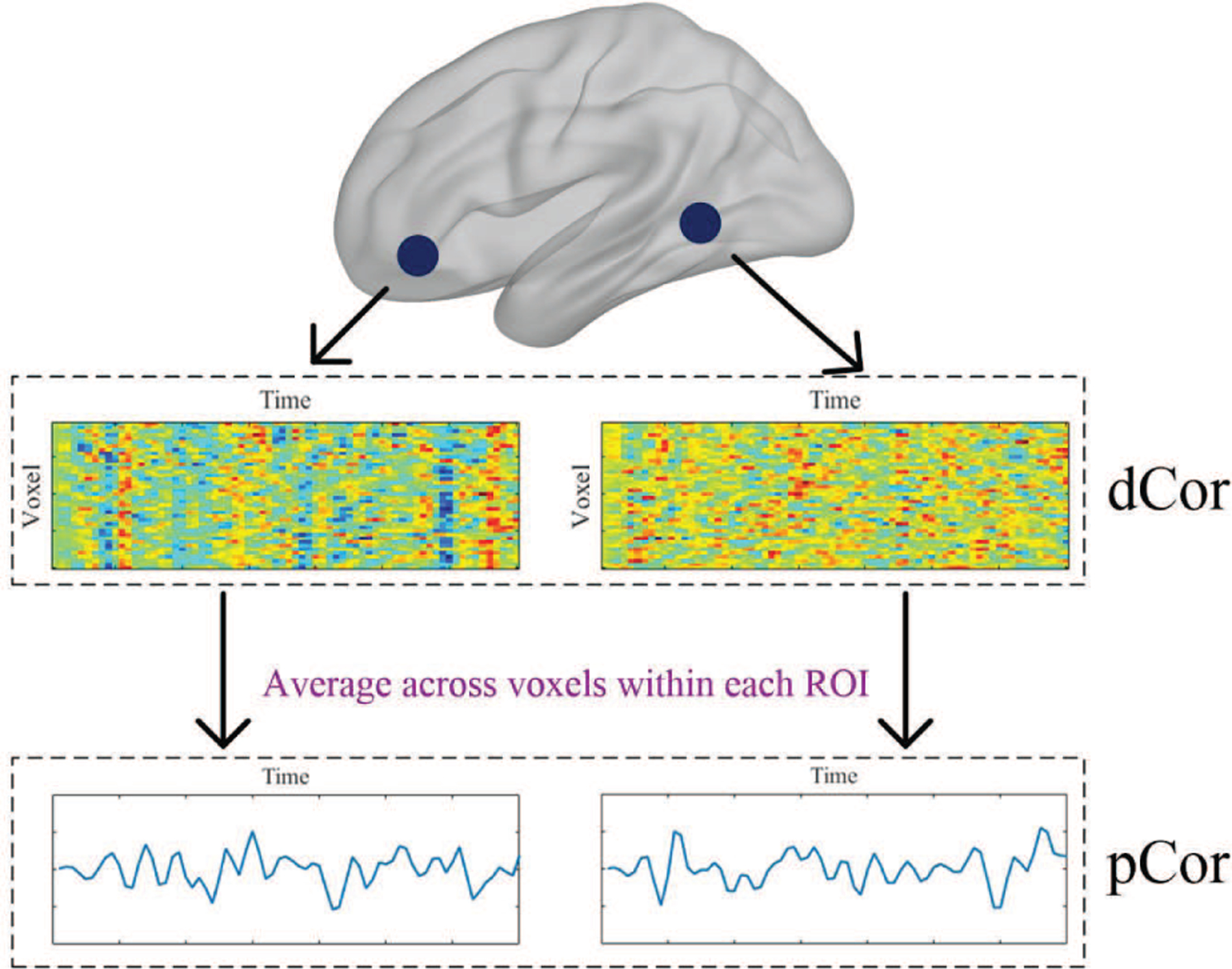
An illustration of the difference between dCor-based FC and pCor-based FC. At the top, each blue dot denotes an ROI; in the middle, each heatmap shows all voxel-wise time courses within the corresponding ROI; at the bottom, each line plot represents an ROI-wise time course calculated by averaging all voxel-wise time courses within the corresponding ROI.
B. Novel non-convex multi-task learning (NC-MTL)
We assume that there are M learning tasks for the data in a d-dimensional feature space. In the i-th task for 1 ≤ i ≤ M, we have a training dataset {Xi, yi}, where is the data matrix with ni training subjects as row vectors, each consisting of d features, and is the corresponding label vector. Let denote the weights of all features to linearly regress the labels yi on Xi in the i-th task. Then, an MTL model for the data can be formulated by the following optimization problem:
| (4) |
Where is the weight matrix of features on all tasks, Ω(W) is the sparsity regularizer imposed for feature selection, and α > 0 is the regularization parameter that balances the tradeoff between residual error and sparsity. Through solving (4), we obtain a sparse weight matrix W* to evaluate the relationship between features and labels, thereby selecting the most discriminative features across all tasks. Note that if the number of tasks equals 1, i.e., M = 1, then becomes the weight vector on one task, and (4) represents single-task learning (STL).
A classical MTL model is to select common features shared by all tasks based on a group sparsity regularizer, i.e., Ω(W) = ∥W∥2,0, in (4). The ℓ2,0 regularizer, extending the ℓ0 regularizer in STL to MTL, penalizes every row of W as a whole, and enforces sparsity among the rows. As the ℓ2,0 regularizer leads to a combinatorially NP-hard optimization problem, its several approximations, such as the ℓ2,p regularizer (i.e.,∥W∥2,p; see Table I) with 0 < p ≤ 1, have been studied. Remarkably, the ℓ2,1 regularizer has been proposed as a convex approximation to the ℓ2,0 regularizer [41]–[43], and MTL in (4) becomes
| (5) |
which performs well and can be easily optimized. On the other hand, as ℓ2,p with 0 < p < 1 is geometrically much closer to ℓ2,0 than ℓ2,1, the ℓ2,p regularizer with 0 < p < 1 has been developed and theoretically proven to outperform the ℓ2,1 regularizer for feature selection [44]–[46]. However, due to the non-convexity and non-Lipschitz continuity of the ℓ2,p regularizer with 0 < p < 1, it is more challenging to solve the optimization problem in MTL. To this end, the non-convex but Lipschitz continuous ℓ2,1−2 regularizer has recently been investigated in [30], which extends the ℓ1−2 regularizer in STL [31]–[33] to MTL, i.e.,
| (6) |
where ∥W∥2,1−2 ≜ ∥W∥2,1 − ∥W∥2,2 = ∥W∥2,1 − ∥W∥F and it is ready to verify ∥W∥2,1−2 ≥ 0 due to ∥W∥F ≤ ∥W∥2,1. The ℓ2,1−2 regularizer has been shown to not only achieve better feature selection performance, but also result in an easier optimization problem because of the Lipschitz continuity.
As we mentioned above, all of the ℓ2,p with 0 < p ≤ 1 and ℓ2,1−2 regularizers are approximations to the ℓ2,0 regularizer in MTL. So, they can only achieve the group sparsity for selecting common features shared by all tasks, but fail to consider task-specific features (i.e., features shared by a subset (but not all) of tasks). To extract both common and task-specific features in MTL, we next introduce a composite of the ℓ2,1−2 and ℓ1−2 regularizers, and obtain the following NC-MTL model:
| (7) |
i.e.,
| (8) |
where ∥W∥1−2 ≜ ∥W∥1 − ∥W∥F is used to enforce the sparsity among all elements in W and we immediately have ∥W∥1−2 ≥ 0 due to ∥W∥F ≤ ∥W∥1. It is worth noting that, the first term ℓ2,1−2 of the composite regularizer in (7) achieves the group sparsity to select common features shared by all tasks, while the second term ℓ1−2 contributes to selecting task-specific features. The two terms are improved alternatives to ℓ2,1 and ℓ1, respectively, which have been adopted in several existing MTL models (see, e.g., [34]–[40]). Hyperparameters α, β > 0 control the balance between the sparsity patterns of common and task-specific features. An illustration of the proposed NC-MTL model is shown in Fig. 2.
Fig. 2:
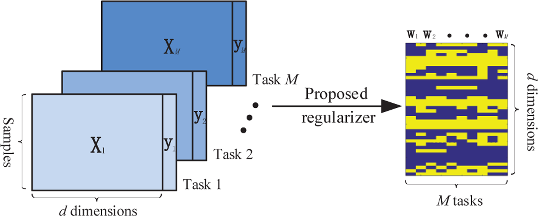
An illustration of the proposed NC-MTL model in (8). The left-hand side shows the input datasets , and the right-hand side shows the sparsity pattern of the learned weight matrix W.
C. Optimization algorithm for NC-MTL
Let us consider the proposed NC-MTL model in (8), whose objective function, denoted as h(W), is non-convex and the subtraction of two convex functions f(W) and g(W), i.e.,
| (9) |
with
| (10) |
| (11) |
A well-known scheme for addressing such a non-convex optimization problem is first to linearize g(W) using its 1st-order Taylor-series expansion at the current solution W(k), and then advance to a new one W(k+1) by solving a convex optimization subproblem in the framework of ConCave-Convex Procedure (CCCP) [47].
More specifically, the CCCP algorithm can solve the above problem (9) with the following iterations.
| (12) |
where S(k) ∈ ∂g(W(k)). Following the definition of sub-gradient, i.e., for any W, g(W(k)) ≥ g(W(k)) + 〈W − W(k),S(k)〉, we obtain
| (13) |
Therefore, the objective function values are monotonically decreasing. Moreover, from the formula of the objective function h(W) in (8), are bounded below by zero, and they thus converge. We can obtain a local optimal W⋆ of (8) by iteratively solving (12); see Algorithm 1 for details.

We next use the accelerated proximal gradient (APG) algorithm [48] to solve the convex subproblem (12) or (14), whose objective function is the summation of two convex functions, i.e., ϕ(W) (differentiable) and φ(W) (non-differentiable) with
| (16) |
| (17) |
Specifically, we iteratively update W as follows.
| (18) |
Where , and l is a variable step size. In matrix calculus, the gradient of a scalar-valued function ϕ(W) with respect to W can be written as a vector whose components are the gradients of ϕ with respect to every column of W. Therefore, we obtain , and for 1 ≤ i ≤ M can be easily calculated as
| (19) |
where wi(t) and s(ik) represent the i-th columns of W(t) and S(k), respectively. Based on simple calculation, we can equivalently rewrite . Then, after ignoring the items independent of W in (18), the update procedure becomes
| (20) |
where V(t) = W(t) − l∇ ϕ(W(t)). Clearly, (20) is in fact,
| (21) |
where proxlφ stands for the proximal operator [49] of the scaled function lφ.

Owing to the separability of W on its rows in (20), we can decouple (20) into the following optimization problem for each row independently, i.e., for 1 ≤ i ≤ d,
| (22) |
where w(t+1),i,wi, and v(t),i represent the i-th rows of W(t+1),W, and V(t), respectively, and τ(wi) = α∥wi∥2+β∥wi∥1 is a function of vector wi. Letting τ1(wi) = β∥wi∥1 and τ2(wi) = α∥wi∥2, we have, from [38], . It is well known that both and have closed-form solutions [49], i.e., with
| (23) |
where ri and ui represent the i-th elements of vectors r and u, respectively, and
| (24) |
Therefore, based on (22)–(24), we can obtain the closed-form solution of W(t+1) in (20). To accelerate the proximal gradient method, we introduce an auxiliary variable as
| (25) |
and perform the gradient descent procedure with respect to Q(t) instead of W(t), where the coefficient θ(t) is updated by
| (26) |
The pseudo-code of the APG algorithm for solving (14) is shown in Algorithm 2.
D. Testing the proposed NC-MTL on synthetic data
We demonstrate the effectiveness of the proposed NC-MTL model in (8) first on synthetic data through a comparison with other competing MTL models. We simulated a dataset with M = 10 tasks and d = 100 features, and each task has 40 samples. We randomly selected 6 features as common features shared by all 10 tasks and 4 features as task-specific features for each task. The weights of the selected features were generated from the uniform distribution 𝒰(1, 3) and the weights of the remaining features were zero (see Fig. 4(a)). The elements of the inputs for 1 ≤ i ≤ 10 were generated from the Gaussian distribution 𝒩(0, 2), and the corresponding label vectors were calculated as yi = Xiwi + ϵi, in which the elements of noise vectors were generated from 𝒩(0,0.1).
Fig. 4:
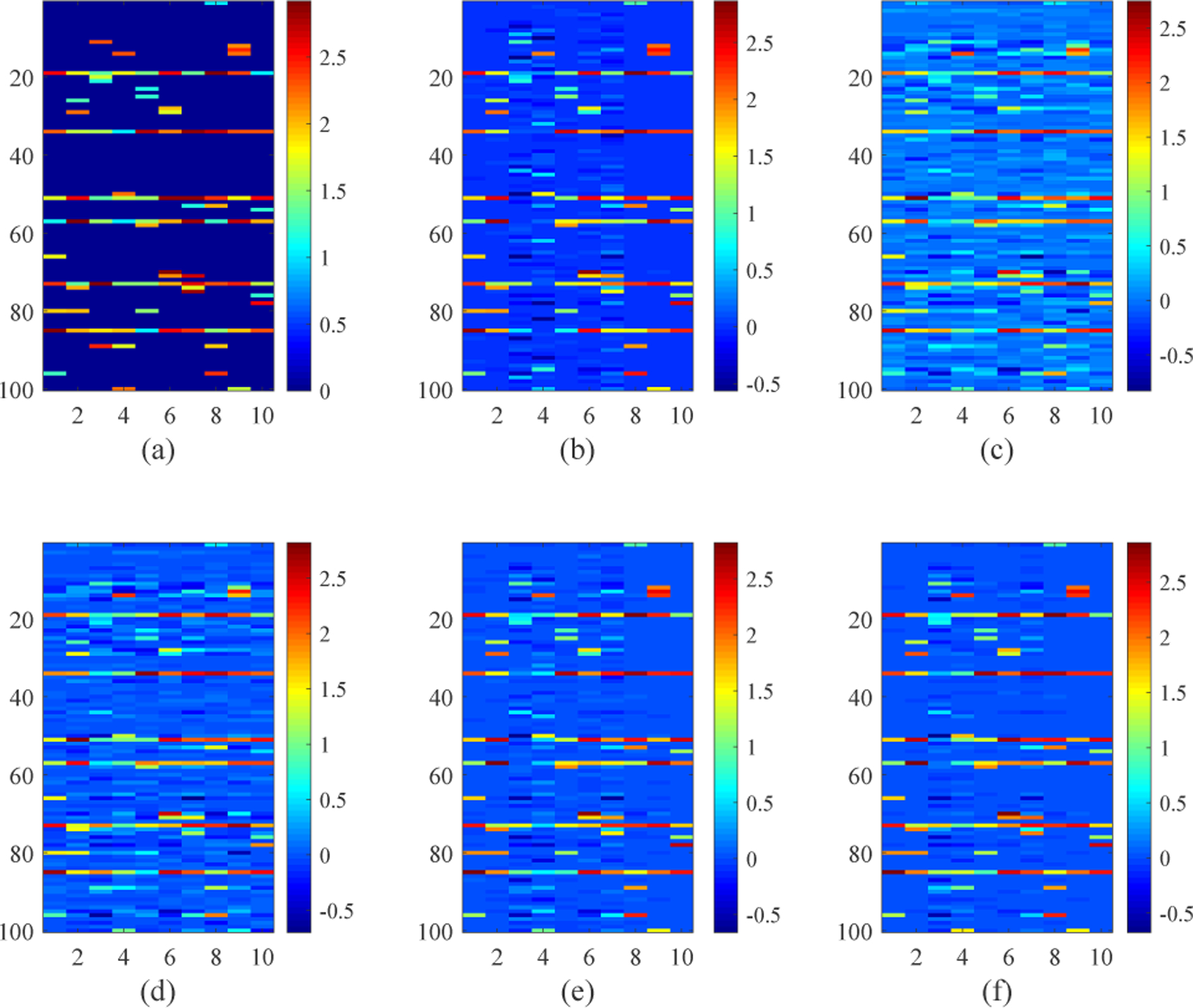
(a) The ground-truth weight matrix . (b)-(f) The average of the learned weight matrices over all runs of CV for each of the five MTL models (i.e., MTL_I, MTL_II, MTL_III, MTL_IV, NC-MTL), respectively.
Based on the simulated data, we compared the performance of our NC-MTL model and the following four popular MTL models.
MTL_I: The model utilizes the ℓ1 regularizer to enforce feature sparsity in MTL, i.e., Ω(W) = ∥W∥1 in (4), which is Lasso in MTL with all tasks sharing the same sparsity parameter.
MTL_II [41]: In the model, the ℓ2,1 regularizer is used to induce the group sparsity in MTL, i.e., Ω(W) = ∥W∥2,1 in (4), for selecting common features shared by all tasks.
MTL_III [30]: The model applies the ℓ2,1−2 regularizer in MTL, i.e., Ω(W) = ∥W∥2,1−2 in (4), which is an improved alternative to the ℓ2,1 regularizer for feature selection.
MTL_IV [34]: In the model, the ℓ2,1 and ℓ1 regularizers are adopted in MTL, i.e., in (4), to select common and task-specific features, respectively.
In Fig. 3, we present the average prediction performance of the five MTL models, which was quantified by using the root mean square error (rmse) for all the test samples of 10 tasks over 10 times 5-fold nested cross-validation (CV, 5-fold CV in the outer loop, and 5-fold CV in the inner loop). The regularization parameters in the MTL models were tuned from the range of {0.1, 0.5, 1, 5, 10, 50, 100, 150, 200, 250, 300}. In Fig. 4(b)–(f), the average of the learned weight matrices over all runs of CV is shown for each MTL model. The difference (in the Frobenius norm) between the averaged learned weight matrix and the ground-truth weight matrix W is 7.7189 for MTL_I, 8.7992 for MTL_II, 7.3381 for MTL_III, 6.6279 for MTL_IV, 4.9697 for NC-MTL. We can observe from Figs. 3 and 4 that the proposed NC-MTL model extracted the most accurate features and achieved the best performance.
Fig. 3:
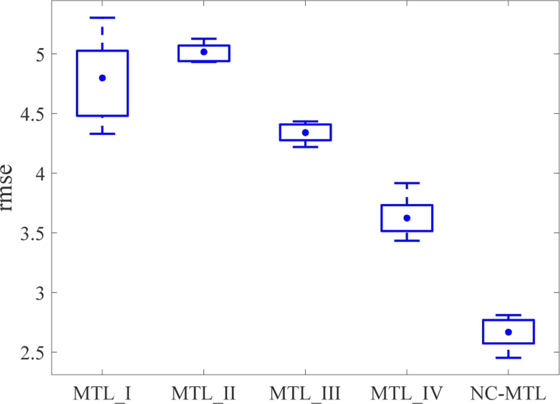
Comparison of the rmse performance of all five MTL models, where box plots show the rmse results with the error bars representing the 25-th and 75-th percentiles, respectively, and the mean values are indicated by •.
Furthermore, we illustrated the performance of the five MTL models in three cases of higher feature dimensionality with d = 500, 1000, 1500. More specifically, we generated the ground-truth weight matrix by randomly incorporating d − 100 all-zero row vectors into the weight matrix as shown in Fig. 4. Accordingly, data and for 1 ≤ i ≤ 10 were simulated and the experimental procedure followed in the same manner as before. In Fig. 5, we present the average prediction performance of the five MTL models in terms of rmse. It demonstrates again superior performance of the proposed NC-MTL model, compared with the other four MTL models.
Fig. 5:
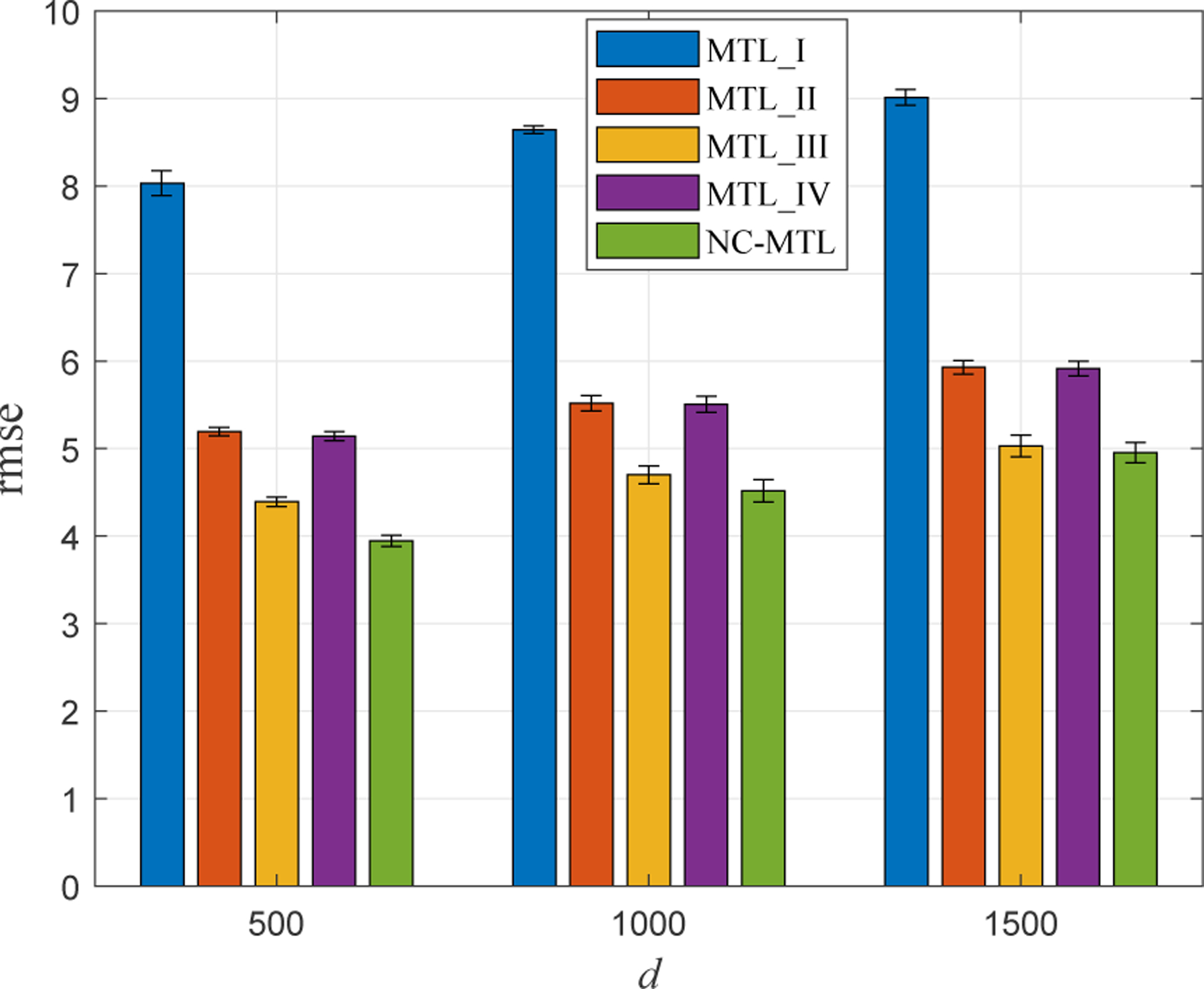
Comparison of the rmse performance of all five MTL models with respect to different numbers of features, i.e., d = 500, 1000, 1500.
III. Experimental Results
A. Data acquisition and preprocessing
In this study, data were taken from the Philadelphia Neurodevelopmental Cohort (PNC) [22], which is a collaborative study of child development between the Brain Behavior Laboratory at the University of Pennsylvania and the Center for Applied Genomics at the Children’s Hospital of Philadelphia. The PNC contained nearly 900 participants (8 – 22 years old) with multimodal neuroimaging and genetics datasets. Our analyses were limited to 715 subjects who underwent rs-fMRI scans and had minimal head movement with a mean frame-wise displacement being less than 0.25 mm. The demographic characteristics of the subjects are presented in Table II. During the resting-state scan, subjects were instructed to stay awake, keep eyes open, fixate on the displayed crosshair, and remain still.
TABLE II:
Demographic characteristics of the subjects in this study; std denotes the standard deviation.
| Male | Female | |
|---|---|---|
| Number of subjects | 319 | 396 |
| Age (range; mean ± std) | 8.58 – 21.75 | 8.67 – 22.58 |
| 15.23 + 3.14 | 15.67 + 3.17 |
All rs-fMRI datasets were acquired on the same 3T Siemens TIM Trio whole-body scanner using a single-shot, interleaved multi-slice, gradient-echo, echo-planar imaging (EPI) sequence (TR/TE = 3000/32 ms, flip angle = 90°, field of view (FOV) = 192 × 192 mm2, matrix = 64 × 64, resolution = 3 × 3 × 3 mm3, and 124 volumes). The scanning duration for each subject was about 6 minutes, resulting in 124 time points. Standard preprocessing procedures were applied to functional images using SPM12 (www.fil.ion.ucl.ac.uk/spm/), which include motion correction, co-registration, spatial normalization to the standard Montreal Neurological Institute (MNI) space, and spatial smoothing with a 3 mm full width half maximum (FWHM) Gaussian kernel. The influences of head motion were regressed out, and functional time courses were band-pass filtered with a passband of 0.01–0.1 Hz. Based on the Power atlas [50], we segmented each subject’s whole-brain into 264 ROIs (modelled as 10 mm diameter spheres), which spanned the cerebral cortex, subcortical structures, and the cerebellum. The majority of these ROIs (227 out of 264) were assigned to 10 pre-defined functional modules, including visual network (VIS), default mode network (DMN), sensory-motor network (SMT), cingulo-opercular network (COP), frontoparietal network (FPT), dorsal attention network (DAT), ventral attention network (VAT), auditory network (AUD), salience network (SAL), and subcortical network (SBC), which were utilized for localization analyses and visualized with BrainNet Viewer [51] in Fig. 6. By computing FC between any pair of ROIs, we obtained a 264×264 FC matrix for each subject. As the FC matrix is symmetric, only its lower triangular portion was unfurled into a feature vector of 34716 FC values for each subject in subsequent analysis.
Fig. 6:
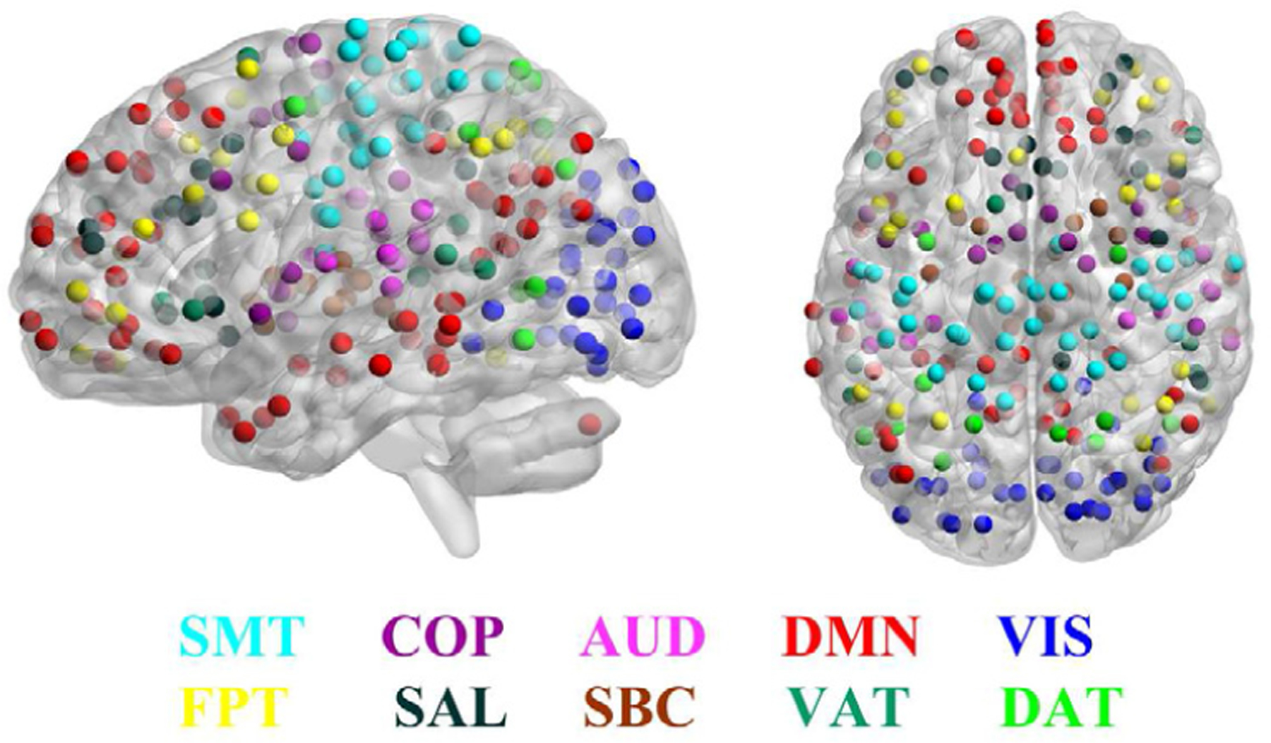
The Power atlas with an a priori assignment of ROIs to different functional modules. ROIs of the same color belong to the same module and ROIs’ colors indicate module memberships, where ROIs assigned to 10 key functional modules were visualized and the others (assigned to cerebellum and unsorted) not.
B. Comparison between pCor-based and dCor-based FC for age prediction in each gender group
In this subsection, for each gender group, we utilized whole-brain FC (i.e., a total of 34716 FC values for each subject) to predict subjects’ ages based on a linear support vector regression (SVR). For comparison, the two different FC estimation methods introduced in Section II-A were employed, resulting in pCor-based and dCor-based FC, respectively. The SVRs (implemented in LIBSVM with default parameters [52]) were trained and tested using 5-fold CV, and the 5-fold CV procedure was repeated 10 times to reduce the effects of sampling bias and provide reliable performance. We reported the average prediction performance, quantified by both correlation coefficient (corr) and rmse between the predicted and observed ages of the subjects in the test sets over all runs of CV.
Fig. 7 illustrates the average dCor-based and pCor-based FC patterns across subjects for each gender group. Due to the symmetry of FC matrices, we respectively visualized the upper triangular portion of the average dCor-based FC matrix and the lower triangular portion of the average pCor-based FC matrix as the upper and lower triangles of a matrix heatmap in Fig. 7. One can see from Fig. 7 that the average dCor-based FC is clearly stronger than the average pCor-based FC. The age prediction performance for each gender group is presented in Fig. 8. More specifically, for the female group, corr and rmse results using dCor-based FC were 0.5891 ± 0.0207 and 2.5662 ± 0.0459, respectively, which were better than those (i.e., 0.5424 ± 0.0169 and 2.6672 ± 0.0306) using pCor-based FC. Similarly, for the male group, the prediction results using dCor-based FC were also better than those using pCor-based FC, i.e., 0.6781 ± 0.0103 and 2.3107 ± 0.0340 vs. 0.6474 ± 0.0118 and 2.3986 ± 0.0407. This suggests that dCor-based FC is more discriminative for age prediction than pCor-based FC. By exploring spatial relations of voxel-wise time courses within individual ROIs, a vector measure of FC can provide more information about brain network organization than a scalar measure of FC. In what follows, we will mainly focus on dCor-based FC for jointly predicting ages of both genders.
Fig. 7:
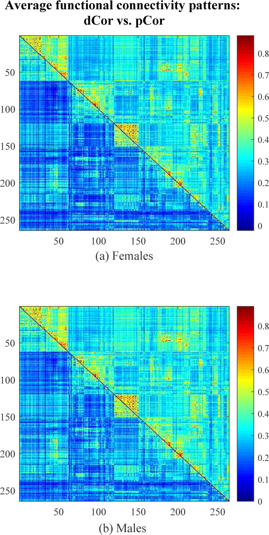
The average FC patterns estimated by dCor (upper triangle of a matrix heatmap) and pCor (lower triangle) across subjects for each gender group.
Fig. 8:
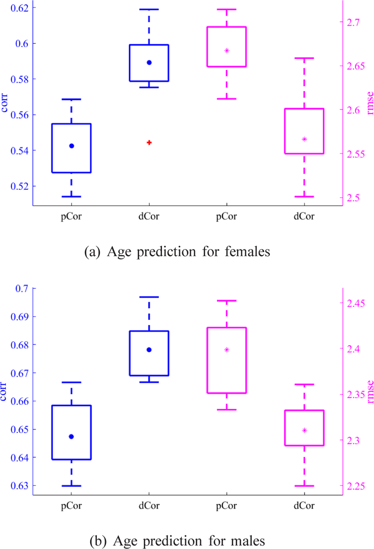
The prediction performance in terms of both corr and rmse for each gender group. Blue box plots exhibit corr results (the higher the better) for the left y-axis, and magenta box plots exhibit rmse results (the lower the better) for the right y-axis, where • and * indicate the corresponding mean values.
C. Results of the proposed NC-MTL for age prediction
In this subsection, with the use of dCor-based FC, we compared the age prediction performance of our NC-MTL model with five other predictive models, i.e., SVR for each gender group separately, and four MTL models (MTL_I, MTL_II, MTL_III, MTL_IV) as mentioned before. We used 10 times 5-fold nested CV to tune the hyperparameters as well as to obtain the best average performance in all experiments. All regularization parameters (also called hyperparameters) in the five MTL models were chosen by a grid search within their respective ranges; that is, α, β ∈ {10−4, 10−3, 10−2, 10−1, 1, 10}. We tuned the penalty parameter C in linear SVR from the range of {2−3, 2−2, 2−1, 1, 2, 4, 8, 16}. Prior to training the predictive models, simple feature filtering was conducted. Specifically, we discarded the dCor-based FC features for which the p-values of the correlation with ages of males and females in the training set were both greater than or equal to 0.01. For each gender group, the remaining features of training subjects were normalized to have zero mean and unit norm, and the mean and norm values of training subjects were used to normalize the corresponding features of testing subjects. We performed the mean-centering on ages of training subjects and then used the mean age value of training subjects to normalize ages of testing subjects.
The detailed age prediction results are summarized in Table III. The accuracy of the proposed NC-MTL model was always superior to those of other predictive models, indicating that our NC-MTL model had better prediction performance. It suggests that the composite regularizer by combining the ℓ2,1−2 and ℓ1−2 regularization terms, introduced in our NC-MTL model, was more effective in identifying discriminative features associated with ages through selecting both common and gender-specific features. Moreover, as shown in Table III, the five MTL models all achieved better prediction performance than the STL model (i.e., SVR), which demonstrates that joint analysis of multiple tasks, while exploiting commonalities and/or differences across them, can result in improved prediction accuracy, compared to learning these tasks independently. For the proposed NC-MTL model, we present the relationships between the predicted and observed ages of males and females in Fig. 9, respectively.
TABLE III:
Comparison of regression performance of the male group and the female group by different predictive models.
| Model | Males | Females | ||
|---|---|---|---|---|
| corr (mean ± std) | rmse (mean ± std) | corr (mean ± std) | rmse (mean ± std) | |
| SVR | 0.6366 ± 0.0172 | 2.4349 ± 0.0420 | 0.5119 ± 0.0215 | 2.7599 ± 0.0449 |
| MTL_I | 0.6432 ± 0.0102 | 2.4239 ± 0.0397 | 0.5140 ± 0.0197 | 2.7560 ± 0.0433 |
| MTL_II | 0.6441 ± 0.0195 | 2.4080 ± 0.0554 | 0.5210 ± 0.0198 | 2.7380 ± 0.0424 |
| MTL_III | 0.6486 ± 0.0083 | 2.3958 ± 0.0222 | 0.5364 ± 0.0181 | 2.6970 ± 0.0382 |
| MTL_IV | 0.6491 ± 0.0183 | 2.3918 ± 0.0517 | 0.5362 ± 0.0183 | 2.6976 ± 0.0386 |
| NC-MTL | 0.6600 ± 0.0096 | 2.3632 ± 0.0318 | 0.5452 ± 0.0164 | 2.6761 ± 0.0358 |
Fig. 9:
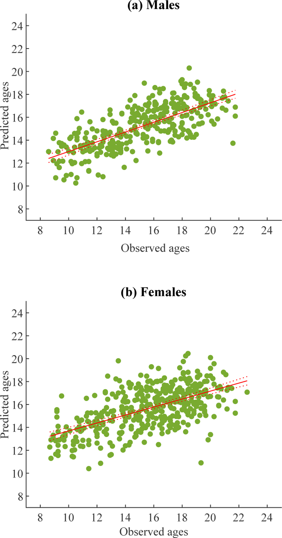
The two scatter plots illustrate the relationships between the predicted and observed ages of males and females, respectively, where the predicted ages were obtained by the proposed NC-MTL model. Each green dot represents one subject. Each red solid line represents the best-fit line of the green dots, and its 95% confidence interval is indicated by two dashed lines.
In the objective function (7) of our NC-MTL model, there are two regularization parameters (i.e., α and β). They balance the relative contributions of the common and task-specific feature selection, respectively. We then studied the effect of these regularization parameters on the age prediction performance. As shown in Fig. 10, the parameters α and β were combined to obtain the age prediction performance of the proposed NC-MTL model, which fluctuates when changing the values of the parameters. One can also see that the optimal values for α and β were α = 1 and β = 1 in both gender groups.
Fig. 10:
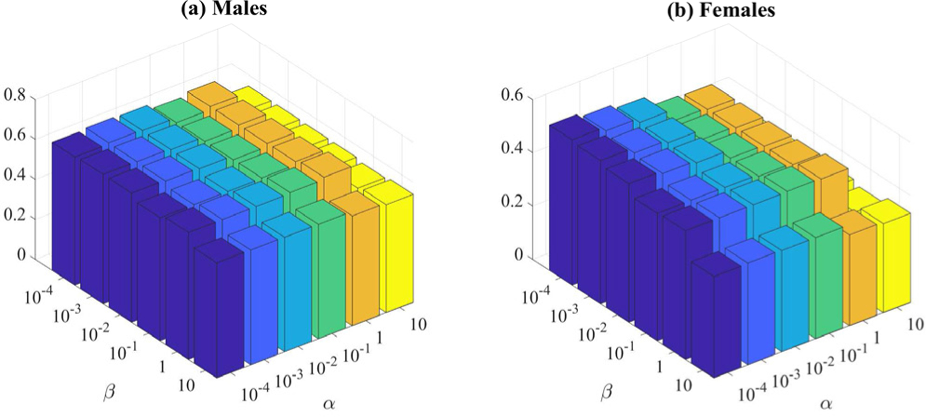
The corr results of both genders based on our NC-MTL model with different values of α and β.
D. Discriminative FC and gender differences detected by the proposed NC-MTL
In this subsection, based on the proposed NC-MTL model, we investigated the most discriminative functional connections (FC features) with potential biological significance relevant to gender differences in brain development. Specifically, the proposed NC-MTL model in (7) generated two weight vectors (i.e., w1 and w2, one for each gender group) of FC features. With respect to each gender group, we averaged the absolute values of the weights of each feature over all runs of CV as the weight of the corresponding FC. The larger the weight of the FC feature is, the more discriminative the FC feature is.
For ease of visualization, we identified the top 150 most discriminative age-related functional connections for each gender group, and Fig. 11 only shows the most discriminative within- and between-module functional connections for the 10 pre-defined functional modules. As shown in Fig. 11, SMT, DMN, VIS, and FPT are important functional modules detected for both genders. The numbers of identified functional connections between SMT and DMN, between FPT and DMN, and within FPT are larger for males. The numbers of identified functional connections between SMT and AUD, within VIS, and between SMT and VIS are larger for females. Functional brain activity spanning the frontoparietal regions were involved in comparing headings, and individual and gender differences were found in the Relative Heading task performance (better for males than females), which may relate to functional differences in relevant brain areas including left lateral orbitofrontal cortex, left precuneus, and right superior parietal [53]. Better navigators have increased functional connections between the right FPT and DMN [54], and the increased functional connections of both parietal and occipital lobes in males may possibly reflect the increased motor and visuospatial skills [55]. Critically, the findings obtained in this paper were consistent with the above results, indicating that males have better spatial orientation and motor coordination skills than females. For females higher connectivity existed between the sensory and attention systems, while for males higher connectivity were observed between the sensory, motor, and default mode systems [56]. There was evidence that FC patterns of the auditory system and many other (e.g., visual and motor) brain systems were related to language-related activation [57]. Therefore, females have better visual language and verbal working memory skills.
Fig. 11:
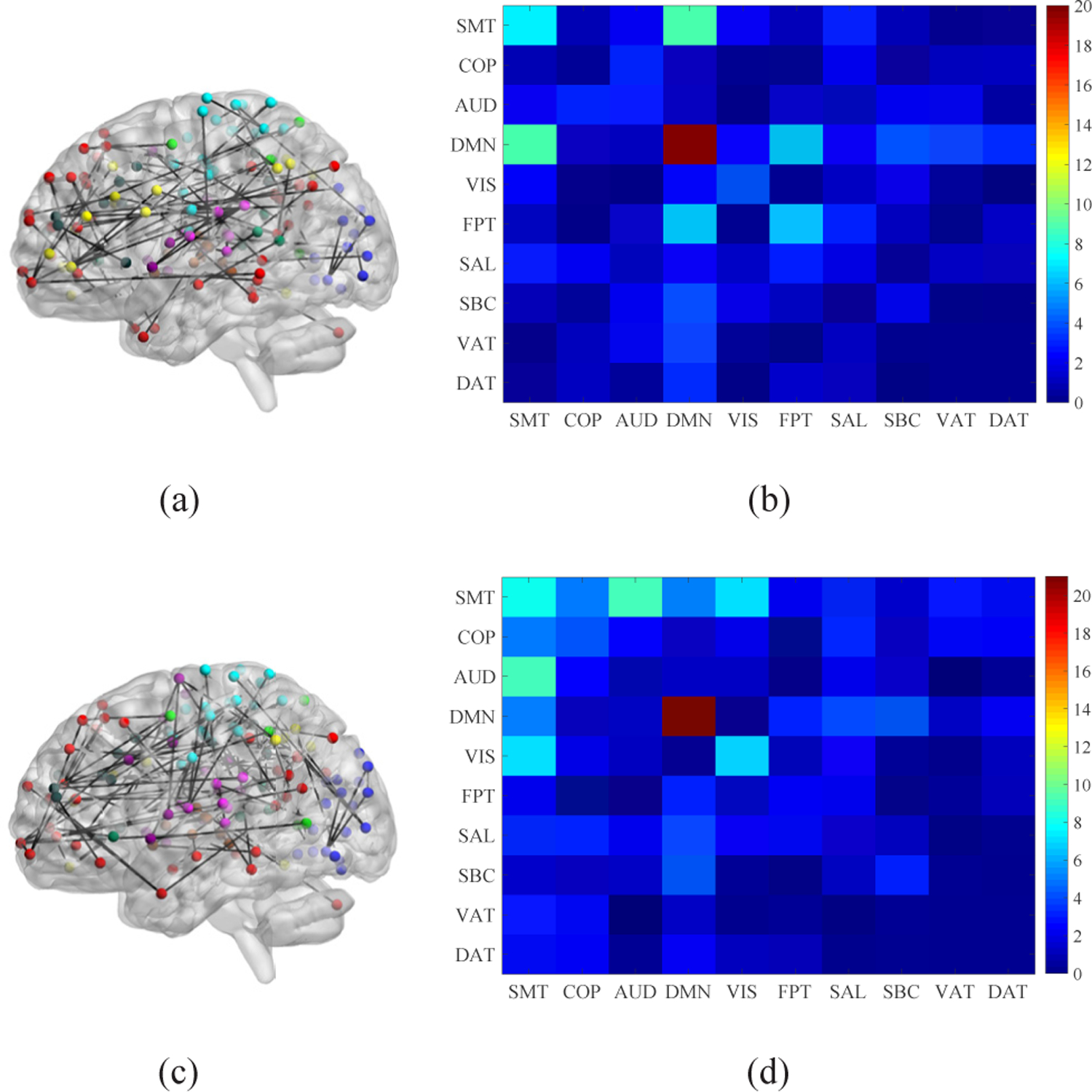
The visualization of the 150 most discriminative age-related functional connections between and within the 10 functional modules for each gender group, i.e., (a)-(b) males and (c)-(d) females. The left are brain plots showing sagittal views of the functional graph in anatomical space, where node colors indicate module membership. The right are matrix plots showing the total numbers of within- and between-module connections.
E. Comparison between the results of the proposed NC-MTL with pCor-based and dCor-based FC for age prediction
Following the same experimental setting as in Subsection III-C, we employed the proposed NC-MTL model with pCor-based FC to jointly predict ages of both genders, and then compared the results with those obtained in Subsection III-C (i.e., the results of the proposed NC-MTL model with dCor-based FC); see Fig. 12. The comparison shown in Fig. 12 suggests again that distance correlation generates more discriminative FC features for age prediction than Pearson’s correlation.
Fig. 12:
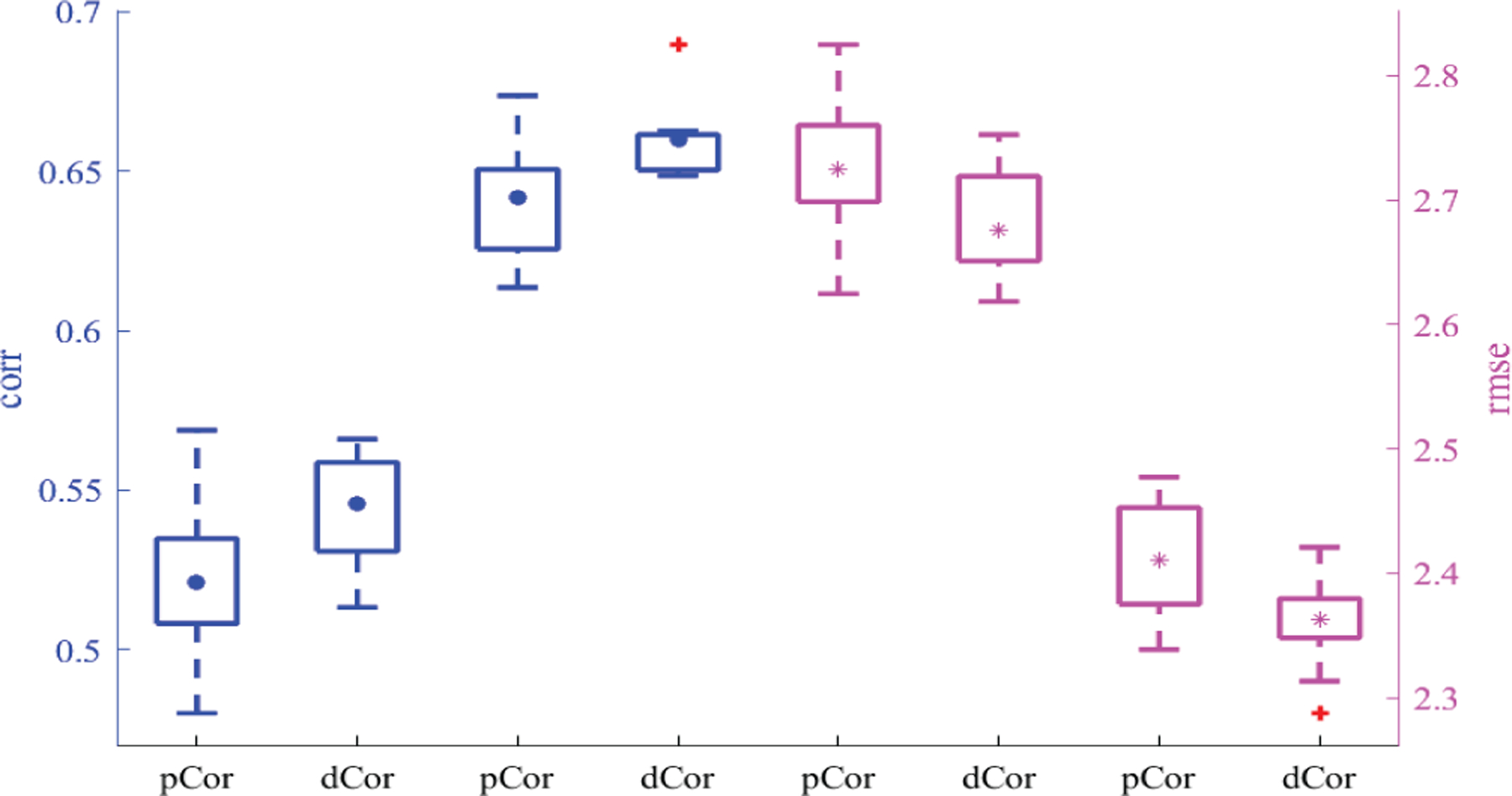
The age prediction performance of the proposed NC-MTL model in terms of both corr and rmse for each gender group. Blue box plots exhibit corr results for the left y-axis, and magenta box plots exhibit rmse results for the right y-axis, where • and * indicate the corresponding mean values, the 1st, 2nd, 5th, and 6th box plots are for females, and the others are for males.
F. Limitations and future work
In this paper, we estimated FC between ROIs using distance correlation rather than Pearson’s correlation. Distance correlation is known as a multivariate statistical method, which is able to measure both linear and nonlinear dependence between ROIs, and therefore captures more complex information. However, like Pearson’s correlation, distance correlation cannot exclude the effects of several other controlling or confounding ROIs when computing pairwise correlations. In our follow-up study, we will take advantage of partial distance correlation [58], [59] and multivariate conditional mutual information [60] to assess conditional dependence between ROIs as FC, and compare their performance with that of distance correlation used in this paper. Although we excluded subjects with high levels of motion to minimize head movement effects in this paper, the confounding of head motion with brain-based age prediction could be significant [17], which should be further taken into consideration for future work. Furthermore, the proposed NC-MTL model achieved satisfactory prediction performance, but we can further improve it. For example, in our NC-MTL model we can impose additional constraints that effectively utilize different pieces of information inherent to the data, such as feature-feature relation, label-label relation, and subject-subject relation [61]. As deep neural networks have recently received increasing attention with demonstrated performance in many applications [62], it will also be interesting to extend the composite regularizer in our NC-MTL model into a multi-task deep learning model. Finally, it will be of interest to apply our NC-MTL model to evaluate differences in FC patterns across different populations, e.g., disease conditions, or developmental stages in behavior and cognition.
The framework proposed in this paper consists of two parts. The first is a dCor-based FC estimation approach that directly uses voxel-wise time courses within each ROI to compute dCor between ROIs as the FC. The second is an NC-MTL model that is applied to jointly predict ages for both gender groups from the FC. The main advantages and disadvantages of our framework as compared to alternatives can be summarized as follows.
As demonstrated in the above experimental results, dCor-based FC was more discriminative for age prediction than pCor-based FC. However, compared with linear dependence that can be simply measured by pCor, nonlinear dependence is rather obscure, and is in general referred to any relationship that is not linear. Therefore, for nonlinear dependence measurement methods including dCor, there is no way to define what a specific nonlinear relationship they capture [63], and as far as we know, there are currently no studies on how much dCor is affected by confounding factors (such as head motion artifacts in dCor-based FC estimation in this paper).
Compared with our NC-MTL model, deep learning-based models can further improve the predictive performance by learning high-level features in a layer-by-layer manner, but they usually demand massive training samples and high computational power in order to optimize a huge number of parameters (i.e., weights and biases of the layers). Moreover, the black-box nature of deep learning models renders them more difficult to identify features or biomarkers for characterizing gender differences in brain development in this paper.
IV. Conclusion
In this paper, we demonstrated that a vector measure of FC can provide more powerful information between ROIs than a scalar measure of FC. The experimental results on the PNC data showed that dCor-based FC better predicted individuals’ ages than pCor-based FC for each gender group. We proposed a novel NC-MTL model by introducing a composite regularizer that combines the ℓ2,1−2 and ℓ1−2 terms, which are improved alternatives to the classical ℓ2,1 and ℓ1 regularization terms, respectively. As a consequence, it leads to improved selection of both common and task-specific features. The experimental results showed improved performance of the proposed NC-MTL model over several other competing ones for jointly predicting ages of both genders using dCor-based FC derived from rs-fMRI, where age prediction for each gender group was viewed as one task. The proposed multi-task model is interpretable, with which we detected both common and gender-specific age-related FC patterns to characterize the effects of gender and age on brain development.
Acknowledgments
This work was supported in part by NIH under Grants R01GM109068, R01MH104680, R01MH107354, R01AR059781, R01EB006841, R01EB005846, R01MH103220, R01MH116782, R01MH121101, P20GM130447, P20GM103472, and in part by NSF under Grant 1539067.
Contributor Information
Li Xiao, Department of Biomedical Engineering, Tulane University, New Orleans, LA 70118.
Biao Cai, Department of Biomedical Engineering, Tulane University, New Orleans, LA 70118.
Gang Qu, Department of Biomedical Engineering, Tulane University, New Orleans, LA 70118.
Gemeng Zhang, Department of Biomedical Engineering, Tulane University, New Orleans, LA 70118.
Julia M. Stephen, Mind Research Network, Albuquerque, NM 87106.
Tony W. Wilson, Department of Neurological Sciences, University of Nebraska Medical Center, Omaha, NE 68198.
Vince D. Calhoun, Tri-Institutional Center for Translational Research in Neuroimaging and Data Science (TReNDS), Georgia State University, Georgia Institute of Technology, Emory University, Atlanta, GA 30030..
Yu-Ping Wang, Department of Biomedical Engineering, Tulane University, New Orleans, LA 70118.
References
- [1].Glover GH, “Overview of functional magnetic resonance imaging,” Neurosurg. Clin. N. Am, vol. 22, pp. 133–139, 2011. [DOI] [PMC free article] [PubMed] [Google Scholar]
- [2].Xu J et al. , “Large-scale functional network overlap is a general property of brain functional organization: Reconciling inconsistent fMRI findings from general-linear-model-based analyses,” Neurosci. Biobehav. Rev, vol. 71, pp. 83–100, 2016. [DOI] [PMC free article] [PubMed] [Google Scholar]
- [3].Biswal BB et al. , “Toward discovery science of human brain function,” Proc. Natl. Acad. Sci, vol. 107, no. 10, pp. 4734–4739, 2010. [DOI] [PMC free article] [PubMed] [Google Scholar]
- [4].Calhoun VD et al. , “Functional brain networks in schizophrenia: A review,” Front. Hum. Neurosci, vol. 3, pp. 1–12, 2009. [DOI] [PMC free article] [PubMed] [Google Scholar]
- [5].Shen X et al. , “Using connectome-based predictive modeling to predict individual behavior from brain connectivity,” Nat. Protoc, vol. 12, no. 3, pp. 506–518, 2017. [DOI] [PMC free article] [PubMed] [Google Scholar]
- [6].Gao S et al. , “Combining multiple connectomes improves predictive modeling of phenotypic measures,” NeuroImage, vol. 201, pp. 116038, 2019. [DOI] [PMC free article] [PubMed] [Google Scholar]
- [7].Jie B et al. , “Integration of network topological and connectivity properties for neuroimaging classification,” IEEE Trans. Biomed. Eng, vol. 61, no. 2, pp. 576–589, 2014. [DOI] [PMC free article] [PubMed] [Google Scholar]
- [8].Finn ES et al. , “Functional connectome fingerprinting: Identifying individuals using patterns of brain connectivity,” Nat. Neurosci, vol. 18, no. 11, pp. 1664, 2015. [DOI] [PMC free article] [PubMed] [Google Scholar]
- [9].Cui Z et al. , “Individual variation in functional topography of association networks in youth,” Neuron, vol. 106, no. 2, pp. 340–353, 2020. [DOI] [PMC free article] [PubMed] [Google Scholar]
- [10].Cai B et al. , “Refined measure of functional connectomes for improved identifiability and prediction,” Hum. Brain Mapp, vol. 40, pp. 4843–4858, 2019. [DOI] [PMC free article] [PubMed] [Google Scholar]
- [11].Fair DA et al. , “Functional brain networks develop from a ‘local to distributed’ organization,” PLoS Comput. Biol, vol. 5, no. 5, pp. e1000381, 2009. [DOI] [PMC free article] [PubMed] [Google Scholar]
- [12].Wang L et al. , “Decoding lifespan changes of the human brain using resting-state functional connectivity MRI,” PLoS ONE, vol. 7, no. 8, pp. e44530, 2012. [DOI] [PMC free article] [PubMed] [Google Scholar]
- [13].Qiu A et al. , “Manifold learning on brain functional networks in aging,” Med. Image Anal, vol. 20, no. 1, pp. 52–60, 2015. [DOI] [PubMed] [Google Scholar]
- [14].Dosenbach NUF et al. , “Prediction of individual brain maturity using fMRI,” Science, vol. 329, no. 5997, pp. 1358–1361, 2010. [DOI] [PMC free article] [PubMed] [Google Scholar]
- [15].Meier TB et al. , “Support vector machine classification and characterization of age-related reorganization of functional brain networks,” NeuroImage, vol. 60, no. 1, pp. 601–613, 2012. [DOI] [PMC free article] [PubMed] [Google Scholar]
- [16].Li H et al. , “Brain age prediction based on resting-state functional connectivity patterns using convolutional neural networks,” in IEEE 15th International Symposium on Biomedical Imaging (ISBI 2018), pp. 101–104, 2018. [DOI] [PMC free article] [PubMed] [Google Scholar]
- [17].Nielsen AN et al. , “Evaluating the prediction of brain maturity from functional connectivity after motion artifact denoising,” Cereb. Cortex, vol. 29, no. 6, pp. 2455–2469, 2019. [DOI] [PMC free article] [PubMed] [Google Scholar]
- [18].Sz´kely GJ et al. , “Measuring and testing dependence by correlation of distances,” Ann. Statist, vol. 35, no. 6, pp. 2769–2794, 2007. [Google Scholar]
- [19].Székely GJ and Rizzo ML, “The distance correlation t-test of independence in high dimension,” J. Multivariate Anal, vol. 117, pp. 193–213, 2013. [Google Scholar]
- [20].Geerligs L et al. , “Functional connectivity and structural covariance between regions of interest can be measured more accurately using multivariate distance correlation,” NeuroImage, vol. 135, pp. 16–31, 2016. [DOI] [PMC free article] [PubMed] [Google Scholar]
- [21].Yoo K et al. , “Multivariate approaches improve the reliability and validity of functional connectivity and prediction of individual behaviors,” NeuroImage, vol. 197, pp. 212–223, 2019. [DOI] [PMC free article] [PubMed] [Google Scholar]
- [22].Satterthwaite TD et al. , “Neuroimaging of the Philadelphia neurodevelopmental cohort,” NeuroImage, vol. 86, pp. 544–553, 2014. [DOI] [PMC free article] [PubMed] [Google Scholar]
- [23].Etchell A et al. , “A systematic literature review of sex differences in childhood language and brain development,” Neuropsychologia, vol. 114, pp. 19–31, 2018. [DOI] [PMC free article] [PubMed] [Google Scholar]
- [24].Schmithorst VJ and Holland SK, “Sex differences in the development of neuroanatomical functional connectivity underlying intelligence found using Bayesian connectivity analysis,” NeuroImage, vol. 35, no. 1, pp. 406–419, 2007. [DOI] [PMC free article] [PubMed] [Google Scholar]
- [25].Zuo X-N et al. , “Growing together and growing apart: Regional and sex differences in the lifespan developmental trajectories of functional homotopy,” J. Neurosci, vol. 30, no. 45, pp. 15034–15043, 2010. [DOI] [PMC free article] [PubMed] [Google Scholar]
- [26].Alarco Gń et al. , “Developmental sex differences in resting state functional connectivity of amygdala sub-regions,” NeuroImage, vol. 115, pp. 235–244, 2015. [DOI] [PMC free article] [PubMed] [Google Scholar]
- [27].Satterthwaite TD et al. , “Linked sex differences in cognition and functional connectivity in youth,” Cereb. Cortex, vol. 25, no. 9, pp. 2383–2394, 2015. [DOI] [PMC free article] [PubMed] [Google Scholar]
- [28].Zhu X et al. , “Parameter-free centralized multi-task learning for characterizing developmental sex differences in resting state functional connectivity,” in Proc. AAAI Conf. Artif. Intell, pp. 2660–2667, 2018. [PMC free article] [PubMed] [Google Scholar]
- [29].Gur RC et al. , “Age group and sex differences in performance on a computerized neurocognitive battery in children age 8–21,” Neuropsychology, vol. 26, no. 2, pp. 251–265, 2012. [DOI] [PMC free article] [PubMed] [Google Scholar]
- [30].Shi Y et al. , “Feature selection with ℓ2,1−2 regularization,” IEEE Trans. Neural Netw. Learn. Syst, vol. 29, no. 10, pp. 4967–4982, 2018. [DOI] [PubMed] [Google Scholar]
- [31].Esser E et al. , “A method for finding structured sparse solutions to nonnegative least squares problems with applications,” SIAM J. Imag. Sci, vol. 6, no. 4, pp. 2010–2046, 2013. [Google Scholar]
- [32].Yin P et al. , “Minimization of ℓ1−2 for compressed sensing,” SIAM J. Sci. Comput, vol. 37, no. 1, pp. A536–A563, 2015. [Google Scholar]
- [33].Lou Y et al. , “Computational aspects of constrained L1 − L2 minimization for compressed sensing,” in Modelling, Computation and Optimization in Information Systems and Management Sciences. Cham, Switzerland: Springer, pp. 169–180, 2015. [Google Scholar]
- [34].Wang H et al. , “Sparse multi-task regression and feature selection to identify brain imaging predictors for memory performance,” in Proc. IEEE Int. Conf. Comput. Vis, pp. 557–562, 2011. [DOI] [PMC free article] [PubMed] [Google Scholar]
- [35].Tabarestani S et al. , “A distributed multitask multimodal approach for the prediction of Alzheimer’s disease in a longitudinal study,” NeuroImage, vol. 206, pp. 116317, 2020. [DOI] [PMC free article] [PubMed] [Google Scholar]
- [36].Brand L et al. , “Joint multi-modal longitudinal regression and classification for Alzheimer’s disease prediction,” IEEE Trans. Med. Imag, vol. 39, no. 6, pp. 1845–1855, 2020. [DOI] [PMC free article] [PubMed] [Google Scholar]
- [37].Xiao L et al. , “A manifold regularized multi-task learning model for IQ prediction from two fMRI paradigms,” IEEE Trans. Biomed. Eng, vol. 67, no. 3, pp. 796–806, 2020. [DOI] [PMC free article] [PubMed] [Google Scholar]
- [38].Zhou J et al. , “Modeling disease progression via fused sparse group lasso,” in Proc. ACM SIGKDD Conf. Knowl. Discovery Data Mining, pp. 1095–1103, 2012. [DOI] [PMC free article] [PubMed] [Google Scholar]
- [39].Wang J et al. , “Sparse multiview task-centralized ensemble learning for ASD diagnosis based on age- and sex-related functional connectivity patterns,” IEEE Trans. Cybern, vol. 49, no. 8, pp. 3141–3154, 2019. [DOI] [PMC free article] [PubMed] [Google Scholar]
- [40].Hao X et al. , “Multi-modal neuroimaging feature selection with consistent metric constant for diagnosis of Alzheimer’s disease,” Med. Image Anal, vol. 60, pp. 101625, 2020. [DOI] [PMC free article] [PubMed] [Google Scholar]
- [41].Argyriou A and Evgeniou T, “Multi-task feature learning,” in Proc. Adv. Neural Inf. Process. Syst, pp. 41–48, 2007. [Google Scholar]
- [42].Nie F et al. , “Efficient and robust feature selection via joint ℓ2,1-norms minimization,” in Proc. Adv. Neural Inf. Process. Syst, pp. 1813–1821, 2010. [Google Scholar]
- [43].Zu C et al. , “Label-aligned multi-task feature learning for multimodal classification of Alzheimer’s disease and mild cognitive impairment,” Brain Imaging Behav, vol. 10, pp. 1148–1159, 2016. [DOI] [PMC free article] [PubMed] [Google Scholar]
- [44].Zhang M et al. , “Feature selection at the discrete limit,” in Proc. AAAI Conf. Artif. Intell, pp. 1355–1361, 2014. [Google Scholar]
- [45].Peng H and Fan Y, “A general framework for sparsity regularized feature selection via iteratively reweighted least square minimization,” in Proc. AAAI Conf. Artif. Intell, pp. 2471–2477, 2017. [Google Scholar]
- [46].Du X et al. , “Multiple graph unsupervised feature selection,” Signal Process, vol. 120, pp. 754–760, 2016. [Google Scholar]
- [47].Yuille AL and Rangarajan A, “The concave-convex procedure,” Neural Comput., vol. 15, no. 4, pp. 915–936, 2003. [DOI] [PubMed] [Google Scholar]
- [48].Nesterov Y, “A method of solving a convex programming problem with convergence rate O(1/k2),” Sov. Math. Doklady, vol. 27, no. 2, pp. 372–376, 1983. [Google Scholar]
- [49].Parikh N and Boyd S, “Proximal algorithms,” Found. Trends Optim, vol. 1, no. 3, pp. 123–231, 2014. [Google Scholar]
- [50].Power JD et al. , “Functional network organization of the human brain,” Neuron, vol. 72, no. 4, pp. 665–678, 2011. [DOI] [PMC free article] [PubMed] [Google Scholar]
- [51].Xia M et al. , “BrainNet Viewer: A network visualization tool for human brain connectomics,” PloS one, vol. 8, no. 7, pp. e68910, 2013. [DOI] [PMC free article] [PubMed] [Google Scholar]
- [52].Chang C-C and Lin C-J, “LIBSVM: a library for support vector machines,” ACM Trans. Intell. Syst. Technol, vol. 2, no. 27, pp. 1–27, 2011. [Google Scholar]
- [53].Burte H et al. , “The neural basis of individual differences in directional sense,” Front. Hum. Neurosci, vol. 12, pp. 410, 2018. [DOI] [PMC free article] [PubMed] [Google Scholar]
- [54].Izen SC et al. , “Resting state connectivity between medial temporal lobe regions and intrinsic cortical networks predicts performance in a path integration task,” Front. Hum. Neurosci, vol. 12, pp. 415, 2018. [DOI] [PMC free article] [PubMed] [Google Scholar]
- [55].Hamilton C, Cognition and Sex Differences. Macmillan International Higher Education, 2008. [Google Scholar]
- [56].Kohls G et al. , “The nucleus accumbens is involved in both the pursuit of social reward and the avoidance of social punishment,” Neuropsychologia, vol. 51, no. 11, pp. 2062–2069, 2013. [DOI] [PMC free article] [PubMed] [Google Scholar]
- [57].Binder JR et al. , “Human brain language areas identified by functional magnetic resonance imaging,” Science, vol. 342, no. 6158, pp. 585–589, 2013. [DOI] [PMC free article] [PubMed] [Google Scholar]
- [58].Székely G and Rizzo ML, “Partial distance correlation with methods for dissimilarities,” Ann. Statist, vol. 42, no. 6, pp. 2382–2412, 2014. [Google Scholar]
- [59].Fang J et al. , “Fast and accurate detection of complex imaging genetics associations based on greedy projected distance correlation,” IEEE Trans. Med. Imag, vol. 37, no. 4, pp. 860–870, 2018. [DOI] [PMC free article] [PubMed] [Google Scholar]
- [60].Sundaram P et al. , “Individual resting-state brain networks enabled by massive multivariate conditional mutual information,” IEEE Trans. Med. Imag, vol. 39, no. 6, pp. 1957–1966, 2020. [DOI] [PMC free article] [PubMed] [Google Scholar]
- [61].Zhu X et al. , “A novel relational regularization feature selection method for joint regression and classification in AD diagnosis,” Med. Image Anal, vol. 38, pp. 205–214, 2017. [DOI] [PMC free article] [PubMed] [Google Scholar]
- [62].Hu W-X et al. , “Interpretable multimodal fusion networks reveal mechanisms of brain cognition,” IEEE Trans. Med. Imag, vol. 40, no. 5, pp. 1474–1483, 2021. [DOI] [PMC free article] [PubMed] [Google Scholar]
- [63].Edelmann D et al. , “On relationships between the Pearson and the distance correlation coefficients,” Stat. Probab. Lett, vol. 169, p. 108960, 2021. [Google Scholar]