Optimal Control Strategy of an Online Game Addiction Model with Incomplete Recovery

Abstract

Since the global COVID-19 pandemic in 2020, some people who have dropped out of online game have become re-addicted to it due to the order of stay-at-home, making the phenomenon of online game addiction even worse. Controlling the prevalence of online game addiction is of great significance to protect people’s healthy life. For this purpose, a mathematical model of online game addiction with incomplete recovery and relapse is established. First, we analyze the basic properties of the model and obtain the expression of the basic reproduction number and all equilibria. By constructing suitable Lyapunov functions, the global asymptotical stability of the equilibria are proved. Then in the numerical simulation, we use the least squares estimation method to fit the real data of e-sports users in China from 2010 to 2020, and obtain the estimated value of all parameters. The approximation value of the basic reproduction number is obtained as $R_0\approx 5.05$. The result reflects that the spread of game addiction in China is very serious. The stability of the equilibria are proved by using the estimated parameter values. Finally, the simulation results between with control and without control during 2020 to 2050 are compared, and the optimal control strategy is found by comparing the total infectious people. The results of optimal control suggest that if we increase our continuous attention to incompletely recovered people, we can prevent more people from becoming addicted to games. The findings in this paper reveal new mechanisms of game addiction transmission and demonstrate a more detailed and reliable control strategy.

Introduction

Since 2020, the coronavirus (COVID-19) pandemic has seriously affected people’s normal life. Stay-at-home commands and isolation increased the consumption of digital amusement, particularly online game and related activities (such as e-sports viewing and video game streaming). For example, Verizon, the US telecoms provider, reported in a report that online game activity increased by 75% during the initial stay-at-home order [7]. According to a report from Italy, web traffic related to the “Fortnite game” increased by 70% during the early stay-at-home order period compared to the previous year [6]. Online games can enrich people’s lives, but excessive gaming can cause many negative effects, including harmful patterns on mental health, sleep, or physical health [21]. It’s also worrisome that the increase in gaming time is causing many of the inadequately recovered game addicts who are in self-quarantine and are undergoing treatment to relapse and become addicted again [10].

Infectious disease dynamics is an important method for theoretical quantitative research. It is based on the characteristics of population growth, the occurrence of diseases, the transmission pattern within the population and related social influence factors to build a reasonable mathematical model to reflect the dynamic changes of infectious diseases [11]. Because of these characteristics, the research methods of infectious disease dynamics have been applied by many scholars to analyze and solve other contagious social problems, such as smoking, alcoholism, drug addiction, game addiction, information diffusion etc. [3, 5, 13, 14, 16–19, 23, 26].

Rahman et al. [19] presented a qualitative analysis of a new smoking model and provided parametric conditions for controlling the influence of smoking. This novel model took into account harmonic mean type incidence rate between the incidence of potential and casual smokers. Ma et al. [17] established and analyzed an alcohol consumption model that considered health education and three time delays. The global dynamic characteristics and control problem of the model with three different time delays are analyzed. Ma et al. [16] proposed a new model of drug transmission that included the influence of media coverage, and analyzed the dynamic behavior to answer the question: Does media coverage affect the transmission of drug addiction? The results showed that the effect of media coverage did not change the stability of drug transmission, but it did affect the number of drug addicts. Li and Guo [14] established a mathematical model of game addiction with a compartment of professional game players for the first time by studying the problem of game addiction in the real world. Through stability analysis and optimal control strategy research, scientific prevention and control suggestions are provided for reducing the number of game addicts. Tian and Ding [26] established a new mathematical model of rumor propagation with rumor refutation behavior, which considered the existence of rumor refutation behavior for the first time, and analyzed the influence of rumor refutation behavior on rumor propagation.

Optimal control theory can be used as a powerful tool to solve the control problem of infectious disease dynamics, and can provide scientific advice for public health administration. Therefore, this method has been widely used in the field of biological mathematics [2, 8, 9, 15, 20, 27, 28, 30]. In [8], the authors developed a Zika virus control model with asymptomatic carriers, taking into account control measures such as mosquito nets, insecticide spraying, and treatment. The numerical solutions with and without control were carried out by the backward Runge–Kutta method. The results of the study provide an optimal control strategy to effectively inhibit the spread of Zika virus. In [28], the authors developed a mathematical model of COVID-19 that took into account an effective contact tracing policy and hospitalization of confirmed cases. In the absence of effective drug interventions, the authors proposed an optimal control strategy to effectively reduce the number of infected persons. In [30], the authors established a stage-structured compartment model in order to study the spread of Huanglongbing. With the aid of optimal control theory, four control methods including spraying insecticide, injecting nutrient solution, cutting down infected trees and setting yellow adhesive traps were considered, and a scientific proposal was put forward to prevent and control the spread of Huanglongbing. There are some other important applications, please see the references.

Some game quitters who are not fully recovered may relapse, fall back into game addiction again, and become addicts. This kind of phenomenon is objective existence, relatively serious, and can not be ignored, especially during home quarantine due to COVID-19 [10]. In order to highlight this phenomenon, we set up a compartment for incompletely recovered quitters when building the model, and there is a certain possibility of recurrence among the population in this compartment.

Based on the above literature and idea, we establish a mathematical model of online game addiction with incompletely recovered quitters, and these incompletely recovered quitters have a certain possibility of relapse. The structure of this paper is as follows. The establishment of the model is shown in Sect. 2, the basic reproduction number and all equilibria of the model are solved in Sect. 3, the stability of the equilibria are proved in Sect. 4, the optimal control problem of the model is analyzed in Sect. 5, and the numerical simulation is studied in Sect. 6.

The Model Formulation

System Description

We divide the total population N(t) into six compartments: susceptible compartment S(t), exposed compartment E(t), infected compartment I(t), professional compartment P(t), the compartment of the incompletely recovered quitters $Q_1(t)$, and the compartment of the completely recovered quitters $Q_2(t)$. Thus, the total population is given by:

$$\begin{array}{c}\hfill N(t)=S(t)+E(t)+I(t)+P(t)+Q_1(t)+Q_2(t).\end{array}$$ 1

S(t): the group of susceptible people who have never been exposed to games;

E(t): the group of exposed people with less exposure to games;

I(t): the group of infected people who are addicted to games;

P(t): the group of professionals who work in professional games or games-related jobs;

$Q_1(t)$: the group of people who were previously addicted to games and now have temporarily withdrawn;

$Q_2(t)$: the group of people who the group of people who quit the game permanently.

In the study of gaming addiction, there exists a group of people who cannot be ignored, who have professional scientific training or who have gaming-related jobs as a profession. Although they have been in contact with games for a very long time, it is not reasonable to classify them in the same category as game addicts. Therefore, we classify people who are professionally involved in gaming as a professional compartment P(t). There are some more descriptions of professional compartment P(t), please see references [5, 14].

There is an important group of game quitters who are influenced by external environmental factors or their own psychological factors and become addicted to games again. This was especially evident during the COVID-19 epidemic, when stay-at-home mandates was imposed in many places [1, 29]. Therefore, we classify these unstable and dissolute dropouts as the incomplete recovery group $Q_1(t)$.

With the rapid development of e-sports, there are more and more e-sports type competitions, many colleges and universities have opened e-sports majors, and many gamers choose to become professional gamers or engage in game-related careers, such as: game designers, game commentators, e-sports tournament hosts, etc [22]. They can go directly from exposed E(t) to professional P(t) without going through the stage of addicted to games. Therefore, we set up a direct connection from E(t) to P(t).

The population flow among those compartments is shown in Fig. 1.

Fig. 1.

Transfer diagram of model

The transfer diagram leads to the following system of ordinary differential equations:

$$\begin{array}{cc}& S^{\prime }(t)=\mu N(t)-\mu S(t)-S(t)\frac{\alpha I(t)+\beta P(t)}{N(t)},\hfill \\ \hfill & E^{\prime }(t)=S(t)\frac{\alpha I(t)+\beta P(t)}{N(t)}-({\xi }_1+{\xi }_2+\mu )E(t),\hfill \\ \hfill & I^{\prime }(t)={\xi }_{1}E(t)+{\delta }_1{Q}_1(t)-(v_1+v_2+v_3+\mu )I(t),\hfill \\ \hfill & P^{\prime }(t)={\xi }_{2}E(t)+v_{1}I(t)-(w_1+w_2+\mu )P(t),\hfill \\ \hfill & Q_1^{\prime }(t)=v_{2}I(t)+w_{1}P(t)-({\delta }_1+{\delta }_2+\mu )Q_1(t),\hfill \\ \hfill & Q_2^{\prime }(t)=v_{3}I(t)+w_{2}P(t)+{\delta }_2{Q}_1(t)-\mu Q_2(t),\hfill \end{array}$$ 2

where

   $\mu$ is the nature birth rate and death rate;

   $\alpha$ denotes the transmission coefficient of the addicted users I;

   $\beta$ is the transmission coefficient of the professional users P;

   ${\xi }_1$ is the transfer rate from E to I;

   ${\xi }_2$ is the transfer rate from E to P;

   $v_1$ represents the transfer rate from I to P;

   $v_2$ represents the proportion of temporarily quit game in I;

   $v_3$ represents the proportion of quit game permanently I;

   $w_1$ represents the proportion of temporarily quit game in P;

   $w_2$ represents the proportion of quit game permanently P;

   ${\delta }_1$ denotes the recurrence rate;

   ${\delta }_2$ denotes the proportion of quit game permanently $Q_1$.

For the convenience of expression, we make some shorthand. $k_1={\xi }_1+{\xi }_2+\mu$, $k_2=v_1+v_2+v_3+\mu$, $k_3=w_1+w_2+\mu$, $k_4={\delta }_1+{\delta }_2+\mu$.

Positivity and Boundedness of Solutions

Since the number of people in each compartment of model (2) is nonnegative and finite, we want to verify here that the solution of model (2) is non-negative and bounded for all $t>0$.

System (2) can be put into the matrix form

$$\begin{array}{c}\hfill X^{\prime }=G(X),\end{array}$$ 3

where $X={(S,E,I,P,Q_1,Q_2)}^{\mathrm{T}}\in R^6$ and G(X) is given by

$$\begin{array}{cc}\hfill G(X)=& \left(\begin{array}{c}{G}_1(X)\\ G_2(X)\\ G_3(X)\\ G_4(X)\\ G_5(X)\\ G_6(X)\end{array}\right)\hfill \\ \hfill =& \left(\begin{array}{c}\mu N-\mu S-S\frac{\alpha I+\beta P}{N}\\ S\frac{\alpha I+\beta P}{N}-k_{1}E\\ {\xi }_{1}E+{\delta }_1{Q}_1-k_{2}I\\ {\xi }_{2}E+v_{1}I-k_{3}P\\ v_{2}I+w_{1}P-k_4{Q}_1\\ v_{3}I+w_{2}P+{\delta }_2{Q}_1-\mu Q_2\end{array}\right).\hfill \end{array}$$ 4

Because of ${\mathrm{\Sigma }}_{i=1}^6{G}_i(X)=0$, N(t) is a constant denoted by N. Letting $\phi (t)=\frac{\alpha I+\beta P}{N}+\mu$, the first equation of system (2) can be written in the following form.

$$\begin{array}{c}\hfill \frac{\mathit{dS}}{\mathit{dt}}=\mu N-\phi (t)S.\end{array}$$

Since the initial values of system (2) are all non-negative, we can obtain the following results by using the integration factor method.

$$\begin{array}{cc}& S(t)=S(0)exp\left(-,{\int }_0^t,\phi ,(u),d,u\right)+exp\left(-,{\int }_0^t,\phi ,(u),d,u\right){\int }_0^t\mu N\left[{\int }_0^x,\phi ,(z),d,z\right]dx\hfill \\ \hfill & >0.\hfill \end{array}$$

For the remaining 5 variables, by a similar method, we can obtain the positivity of the solution. We set

$$\begin{array}{c}\hfill \mathrm{\Omega }=\left\{\left(S,,,E,,,I,,,P,,,Q_1,,,Q_2\right),\in ,R_{+}^6,:,S,+,E,+,I,+,P,+,Q_1,+,Q_2,=,N\right\},\end{array}$$ 5

and it is a positive invariant set of system (2).

The Basic Reproduction Number and Existence of Addiction-Present Equilibrium

The Basic Reproduction Number

The model has an addiction-free equilibrium $D_0$ given by

$$\begin{array}{c}\hfill D_0=(N,0,0,0,0,0).\end{array}$$ 6

In the following, the basic reproduction number of system (2) will be obtained by the next generation matrix method. Let $x={(E,I,P,Q_1,Q_2,S)}^{\mathrm{T}}$, then system(2) can be written as

$$\begin{array}{c}\hfill \frac{\mathit{dx}}{\mathit{dt}}=\mathcal{F}(x)-\mathcal{V}(x).\end{array}$$ 7

where

$$\begin{array}{c}\hfill \mathcal{F}(x)=\left(\begin{array}{c}S\frac{\alpha I+\beta P}{N}\\ 0\\ 0\\ 0\\ 0\\ 0\end{array}\right),\mathcal{V}(x)=\left(\begin{array}{c}{k}_1{E}_1\\ -{\xi }_{1}E-{\delta }_1{Q}_1+k_{2}I\\ -{\xi }_{2}E-v_{1}I+k_{3}P\\ -v_{2}I-w_{1}P+k_4{Q}_1\\ -v_{3}I-w_{2}P-{\delta }_2{Q}_1+\mu Q_2\\ -\mu N+\mu S+S\frac{\alpha I+\beta P}{N}\end{array}\right).\end{array}$$

The Jacobian matrices of $\mathcal{F}(x)$ and $\mathcal{V}(x)$ at the addiction-free equilibrium $D_0$ are

$$\begin{array}{c}\hfill D\mathcal{F}(D_0)=\left(\begin{array}{cc}{F}_{4\times 4}& 0\\ 0& 0\end{array}\right),D\mathcal{V}(D_0)=\left(\begin{array}{cc}{V}_{4\times 4}& 0\\ J_1& J_2\end{array}\right).\end{array}$$

where

$$\begin{array}{cc}\hfill F_{4\times 4}=& \left(\begin{array}{cccc}0& \alpha & \beta & 0\\ 0& 0& 0& 0\\ 0& 0& 0& 0\\ 0& 0& 0& 0\end{array}\right),V_{4\times 4}=\left(\begin{array}{cccc}{k}_1& 0& 0& 0\\ -{\xi }_1& k_2& 0& -{\delta }_1\\ -{\xi }_2& -v_1& k_3& 0\\ 0& -v_2& -w_1& k_4\end{array}\right).\hfill \\ \hfill J_1=& \left(\begin{array}{cccc}0& -v_3& -w_2& -{\delta }_2\\ 0& \alpha & \beta & 0\end{array}\right),J_2=\left(\begin{array}{cc}\mu & 0\\ 0& \mu \end{array}\right).\hfill \end{array}$$

Following Diekmann et al. [4], we can obtain the expression for the basic reproduction number from the spectral radius of $F{V}^{-1}$.

$$\begin{array}{c}\hfill R_0=\rho \left(F,V^{-1}\right)=\frac{\alpha {\xi }_1{k}_3{k}_4+\alpha {\delta }_1{\xi }_2{w}_1+\beta {\xi }_2{k}_2{k}_4+\beta {\xi }_1{v}_1{k}_4-\beta {\delta }_1{\xi }_2{v}_2}{k_1{k}_2{k}_3{k}_4-{\delta }_1{v}_2{k}_1{k}_3-{\delta }_1{v}_1{w}_1{k}_1},\end{array}$$

where $\rho (A)$ denotes the spectral radius of a matrix A.

Since $\beta {\xi }_2(k_2{k}_4-{\delta }_1{v}_2)$ is greater than 0, the numerator of $R_0$ is greater than 0. In the denominator of $R_0$, we get that

$$\begin{array}{cc}& k_1{k}_2{k}_3{k}_4-{\delta }_1{v}_2{k}_1{k}_3-{\delta }_1{v}_1{w}_1{k}_1\hfill \\ \hfill & >k_1{k}_2{k}_3{k}_4-{\delta }_1{v}_2{k}_1{k}_3-{\delta }_1{v}_1{k}_3{k}_1\hfill \\ \hfill & =k_1{k}_3(k_2{k}_4-{\delta }_1{v}_2-{\delta }_1{v}_1)\hfill \\ \hfill & >k_1{k}_3(k_2{k}_4-{\delta }_1{k}_2)\hfill \\ \hfill & >0.\hfill \end{array}$$

Therefore, the basic reproduction number $R_0$ is always positive.

Existence of Addiction-Present Equilibrium

The addiction-present equilibrium $D^{\ast }\left(S^{\ast },,,E^{\ast },,,I^{\ast },,,P^{\ast },,,Q_1^{\ast },,,Q_2^{\ast }\right)$ of system (2) is determined by equations:

$$\begin{array}{cc}& \mu N-\mu S-S\frac{\alpha I+\beta P}{N}=0,\hfill \end{array}$$ 8

$$\begin{array}{cc}& S\frac{\alpha I+\beta P}{N}-k_{1}E=0,\hfill \end{array}$$ 9

$$\begin{array}{cc}& {\xi }_{1}E+{\delta }_1{Q}_1-k_{2}I=0,\hfill \end{array}$$ 10

$$\begin{array}{cc}& {\xi }_{2}E+v_{1}I-k_{3}P=0,\hfill \end{array}$$ 11

$$\begin{array}{cc}& v_{2}I+w_{1}P-k_4{Q}_1=0,\hfill \end{array}$$ 12

$$\begin{array}{cc}& v_{3}I+w_{2}P+{\delta }_2{Q}_1-\mu Q_2=0.\hfill \end{array}$$ 13

Through the above equations we can have $D^{\ast }\left(S^{\ast },,,E^{\ast },,,I^{\ast },,,P^{\ast },,,Q_1^{\ast },,,Q_2^{\ast }\right)$.

Theorem 3.1

In the model (2), there is always an addiction-free equilibrium $D_0=(N,0,0,0,0,0)$. When $R_0>1$, the model has a unique addiction-present equilibrium $D^{\ast }\left(S^{\ast },,,E^{\ast },,,I^{\ast },,,P^{\ast },,,Q_1^{\ast },,,Q_2^{\ast }\right)$, where

$$\begin{array}{cc}& S^{\ast }=\frac{N}{R_0},\hfill \\ \hfill & E^{\ast }=\frac{\mu N}{k_1}\left(1,-,\frac{1}{R_0}\right),\hfill \\ \hfill & I^{\ast }=\frac{\mu N({\xi }_1{k}_3{k}_4+{\xi }_2{\delta }_1{w}_1)}{k_1{k}_2{k}_3{k}_4-{\delta }_1{v}_2{k}_1{k}_3-{\delta }_1{v}_1{w}_1{k}_1}\left(1,-,\frac{1}{R_0}\right),\hfill \\ \hfill & P^{\ast }=\frac{\mu N\left({\xi }_1,v_1,k_4,+,{\xi }_2,k_2,k_4,-,{\xi }_2,{\delta }_1,v_2\right)}{k_1{k}_2{k}_3{k}_4-{\delta }_1{v}_2{k}_1{k}_3-{\delta }_1{v}_1{w}_1{k}_1}\left(1,-,\frac{1}{R_0}\right),\hfill \\ \hfill & Q_1^{\ast }=\frac{\mu N\left(w_1,{\xi }_1,v_1,+,w_1,{\xi }_2,k_2,+,v_2,{\xi }_1,k_3\right)}{k_1{k}_2{k}_3{k}_4-{\delta }_1{v}_2{k}_1{k}_3-{\delta }_1{v}_1{w}_1{k}_1}\left(1,-,\frac{1}{R_0}\right),\hfill \\ \hfill & Q_2^{\ast }=N(\frac{v_3{\xi }_1{k}_3{k}_4+v_3{\xi }_2{\delta }_1{w}_1+w_2{\xi }_1{v}_1{k}_4+w_2{\xi }_2{k}_2{k}_4-w_2{\xi }_2{\delta }_1{v}_2+w_1{\xi }_1{\delta }_2{v}_1}{k_1{k}_2{k}_3{k}_4-{\delta }_1{v}_2{k}_1{k}_3-{\delta }_1{v}_1{w}_1{k}_1}\hfill \\ \hfill & +\frac{{\delta }_2{v}_2{\xi }_1{k}_3+{\delta }_2{w}_1{\xi }_2{k}_2}{k_1{k}_2{k}_3{k}_4-{\delta }_1{v}_2{k}_1{k}_3-{\delta }_1{v}_1{w}_1{k}_1})\left(1,-,\frac{1}{R_0}\right).\hfill \end{array}$$

Stability Analysis of Equilibria

Theorem 4.1

For the system (2), the addiction-free equilibrium $D_0$ is globally asymptotically stable (GAS) if $R_0<1$.

Proof

In order to construct a Lyapunov function, let’s first prove that $k_1{k}_3-\beta {\xi }_2$ is positive. When $0<R_0<1$,

$$\begin{array}{cc}& \alpha ({\xi }_1{k}_3{k}_4+{\delta }_1{\xi }_2{w}_1)+\beta k_4({\xi }_2{k}_2+{\xi }_1{v}_1)-\beta {\delta }_1{\xi }_2{v}_2\hfill \\ \hfill & <k_1(k_2{k}_3{k}_4-{\delta }_1{v}_2{k}_3-{\delta }_1{v}_1{w}_1),\hfill \\ \hfill & \alpha ({\xi }_1{k}_3{k}_4+{\delta }_1{\xi }_2{w}_1)+\beta {\xi }_1{v}_1{k}_4+{\delta }_1{v}_1{w}_1{k}_1<(k_1{k}_3-\beta {\xi }_2)(k_2{k}_4-{\delta }_1{v}_2).\hfill \end{array}$$

Due to $\alpha \left({\xi }_1,k_3,k_4,+,{\delta }_1,{\xi }_2,w_1\right)+\beta {\xi }_1{v}_1{k}_4+{\delta }_1{v}_1{w}_1{k}_1>0$ and $k_2{k}_4-{\delta }_1{v}_2>0$, $k_1{k}_3-\beta {\xi }_2$ is positive. Thus, we can introduce the Lyapunov function V as follows:

$$\begin{array}{c}\hfill V(t)=\frac{{\xi }_1{k}_3{k}_4+{\delta }_1{w}_1{\xi }_2}{k_1{k}_3{k}_4-\beta {\xi }_2{k}_4}{E}_1(t)+I(t)+\left(\frac{\beta }{k_3},\frac{{\xi }_1{k}_3{k}_4+{\delta }_1{w}_1{\xi }_2}{k_1{k}_3{k}_4-\beta {\xi }_2{k}_4},+,\frac{{\delta }_1{w}_1}{k_3{k}_4}\right)P+\frac{{\delta }_1}{k_4}{Q}_1.\end{array}$$

So

$$\begin{array}{cc}\hfill V^{\prime }(t)=& \frac{{\xi }_1{k}_3{k}_4+{\delta }_1{w}_1{\xi }_2}{k_1{k}_3{k}_4-\beta {\xi }_2{k}_4}\left(S,\frac{\alpha I+\beta P}{N},-,k_1,E\right)+{\xi }_{1}E+{\delta }_1{Q}_1-k_{2}I\hfill \\ \hfill & +(\frac{\beta }{k_3}\frac{{\xi }_1{k}_3{k}_4+{\delta }_1{w}_1{\xi }_2}{k_1{k}_3{k}_4-\beta {\xi }_2{k}_4}+\frac{{\delta }_1{w}_1}{k_3{k}_4})\left({\xi }_2,E,+,v_1,I,-,k_3,P\right)\hfill \\ \hfill & +\frac{{\delta }_1}{k_4}\left(v_2,I,+,w_1,P,-,k_4,Q_1\right)\hfill \\ \hfill <& \frac{{\xi }_1{k}_3{k}_4+{\delta }_1{w}_1{\xi }_2}{k_1{k}_3{k}_4-\beta {\xi }_2{k}_4}\left(\alpha ,I,+,\beta ,P,-,k_1,E\right)+{\xi }_{1}E+{\delta }_1{Q}_1-k_{2}I\hfill \\ \hfill & +(\frac{\beta }{k_3}\frac{{\xi }_1{k}_3{k}_4+{\delta }_1{w}_1{\xi }_2}{k_1{k}_3{k}_4-\beta {\xi }_2{k}_4}+\frac{{\delta }_1{w}_1}{k_3{k}_4})\left({\xi }_2,E,+,v_1,I,-,k_3,P\right)\hfill \\ \hfill & +\frac{{\delta }_1}{k_4}(v_{2}I+w_{1}P-k_4{Q}_1)\hfill \\ \hfill =& E[-\frac{{\xi }_1{k}_1{k}_3{k}_4+{\delta }_1{w}_1{\xi }_2{k}_1}{k_1{k}_3{k}_4-\beta {\xi }_2{k}_4}+{\xi }_1+(\frac{\beta }{k_3}\frac{{\xi }_1{k}_3{k}_4+{\delta }_1{w}_1{\xi }_2}{k_1{k}_3{k}_4-\beta {\xi }_2{k}_4}+\frac{{\delta }_1{w}_1}{k_3{k}_4}){\xi }_2]\hfill \\ \hfill & +I[\frac{\alpha {\xi }_1{k}_3{k}_4+\alpha {\delta }_1{w}_1{\xi }_2}{k_1{k}_3{k}_4-\beta {\xi }_2{k}_4}-k_2+(\frac{\beta }{k_3}\frac{{\xi }_1{k}_3{k}_4+{\delta }_1{w}_1{\xi }_2}{k_1{k}_3{k}_4-\beta {\xi }_2{k}_4}+\frac{{\delta }_1{w}_1}{k_3{k}_4})v_1+\frac{{\delta }_1{v}_2}{k_4}]\hfill \\ \hfill & +P[\frac{\beta {\xi }_1{k}_3{k}_4+\beta {\delta }_1{w}_1{\xi }_2}{k_1{k}_3{k}_4-\beta {\xi }_2{k}_4}-(\frac{\beta }{k_3}\frac{{\xi }_1{k}_3{k}_4+{\delta }_1{w}_1{\xi }_2}{k_1{k}_3{k}_4-\beta {\xi }_2{k}_4}+\frac{{\delta }_1{w}_1}{k_3{k}_4})k_3+\frac{{\delta }_1{w}_1}{k_4}]\hfill \\ \hfill =& \frac{I}{k_1{k}_3{k}_4-\beta {\xi }_2{k}_4}[\alpha {\xi }_1{k}_3{k}_4+\alpha {\delta }_1{w}_1{\xi }_2-k_1{k}_2{k}_3{k}_4+\beta {\xi }_2{k}_2{k}_4\hfill \\ \hfill & +\frac{\beta }{k_3}\left(v_1,{\xi }_1,k_3,k_4,+,v_1,{\delta }_1,w_1,{\xi }_2\right)+\frac{{\delta }_1{w}_1{v}_1}{k_3{k}_4}(k_1{k}_3{k}_4-\beta {\xi }_2{k}_4)\hfill \\ \hfill & +\frac{{\delta }_1{v}_2}{k_4}(k_1{k}_3{k}_4-\beta {\xi }_2{k}_4)]\hfill \\ \hfill =& \frac{I}{k_1{k}_3{k}_4-\beta {\xi }_2{k}_4}[\alpha {\xi }_1{k}_3{k}_4+\alpha {\delta }_1{w}_1{\xi }_2+\beta {\xi }_2{k}_2{k}_4+\beta v_1{\xi }_1{k}_4-\beta {\delta }_1{\xi }_2{v}_2\hfill \\ \hfill & -(k_1{k}_2{k}_3{k}_4-{\delta }_1{v}_2{k}_1{k}_3-{\delta }_1{w}_1{v}_1{k}_1)]\hfill \\ \hfill =& \frac{I}{k_1{k}_3{k}_4-\beta {\xi }_2{k}_4}(k_1{k}_2{k}_3{k}_4-{\delta }_1{v}_2{k}_1{k}_3-{\delta }_1{w}_1{v}_1{k}_1)(R_0-1).\hfill \end{array}$$

It can be shown that $V^{\prime }(t)<0$ if $R_0<1$, and $V^{\prime }(t)=0$ if $I=0$. So we can get that $V^{\prime }(t)\le 0$, and the addiction-free equilibrium $D_0$ is the singleton largest compact invariant set in $\mathrm{\Omega }$. Due to the LaSalle’s Invariance Principle [11], the addiction-free equilibrium $D_0$ is globally asymptotically stable. $\square$

Theorem 4.2

 For the system (2), the addiction-present equilibrium $D^{\ast }=(S^{\ast },E^{\ast },I^{\ast },P^{\ast },Q_1^{\ast },Q_2^{\ast })$ is globally asymptotically stable if $R_0>1$.

Proof

First, let’s make the following variable substitution. By denoting

$$\begin{array}{c}\hfill x=\frac{S}{S^{\ast }},y=\frac{E}{E^{\ast }},z=\frac{I}{I^{\ast }},m=\frac{P}{P^{\ast }},n=\frac{Q_1}{Q_1^{\ast }}.\end{array}$$

We have

$$\begin{array}{cc}& \frac{\mathit{dx}}{\mathit{dt}}=x\left[\frac{\mu N}{S^{\ast }},\left(\frac{1}{x},-,1\right),-,\alpha ,\frac{I^{\ast }}{N},(z-1),-,\beta ,\frac{P^{\ast }}{N},(m-1)\right],\hfill \\ \hfill & \frac{\mathit{dy}}{\mathit{dt}}=y\left[{\alpha }_1,\frac{S^{\ast }{I}^{\ast }}{E^{\ast }N},\left(\frac{\mathit{xz}}{y},-,1\right),+,\beta ,\frac{S^{\ast }{P}^{\ast }}{E^{\ast }N},\left(\frac{\mathit{xm}}{y},-,1\right)\right],\hfill \\ \hfill & \frac{\mathit{dz}}{\mathit{dt}}=z\left[{\xi }_1,\frac{E^{\ast }}{I^{\ast }},\left(\frac{y}{z},-,1\right),+,{\delta }_1,\frac{Q_1^{\ast }}{I^{\ast }},\left(\frac{n}{z},-,1\right)\right],\hfill \\ \hfill & \frac{\mathit{dm}}{\mathit{dt}}=m\left[{\xi }_2,\frac{E^{\ast }}{P^{\ast }},\left(\frac{y}{m},-,1\right),+,v_1,\frac{I^{\ast }}{P^{\ast }},\left(\frac{z}{m},-,1\right)\right],\hfill \\ \hfill & \frac{\mathit{dn}}{\mathit{dt}}=n\left[v_2,\frac{I^{\ast }}{Q_1^{\ast }},\left(\frac{z}{n},-,1\right),+,w_1,\frac{P^{\ast }}{Q_1^{\ast }},\left(\frac{m}{n},-,1\right)\right].\hfill \end{array}$$

Therefore, we can see that the addiction-present equilibrium $D^{\ast }$ of system (2) is transformed into ${\overline{D}}^{\ast }=(1,1,1,1,1,1)$. Setting a Lyapunov function V as follows:

$$\begin{array}{cc}\hfill V=& a_1{S}^{\ast }(x-1-lnx)+a_2{E}^{\ast }(y-1-lny)+a_3{I}^{\ast }(z-1-lnz)\hfill \\ \hfill & +a_4{P}^{\ast }(m-1-lnm)+a_5{Q}_1^{\ast }(n-1-lnn),\hfill \end{array}$$

where $a_1$, $a_2$, $a_3$, $a_4$ and $a_5$ are undetermined positive coefficients. We obtain the derivative of V as follows:

$$\begin{array}{cc}\hfill V^{\prime }=& a_1{S}^{\ast }\left(1,-,\frac{1}{x}\right)x^{\prime }+a_2{E}^{\ast }\left(1,-,\frac{1}{y}\right)y^{\prime }+a_3{I}^{\ast }\left(1,-,\frac{1}{z}\right)z^{\prime }+a_4{P}^{\ast }\left(1,-,\frac{1}{m}\right)m^{\prime }\hfill \\ \hfill & +a_5{Q}_1^{\ast }\left(1,-,\frac{1}{n}\right)n^{\prime }\hfill \\ \hfill =& a_1\left(2,\mu ,N,-,S^{\ast },\frac{\alpha I^{\ast }}{N},-,S^{\ast },\frac{\beta P^{\ast }}{N}\right)+a_2\left(S^{\ast },\frac{\alpha I^{\ast }}{N},+,S^{\ast },\frac{\beta P^{\ast }}{N}\right)+a_3\left({\xi }_1,E^{\ast },+,{\delta }_1,Q_1^{\ast }\right)\hfill \\ \hfill & +a_4\left({\xi }_2,E^{\ast },+,v_1,I^{\ast }\right)+a_5\left(v_2,I^{\ast },+,w_1,P^{\ast }\right)-\left(a_1,\mu ,N,-,a_1,S^{\ast },\frac{\alpha I^{\ast }}{N},-,a_1,S^{\ast },\frac{\beta P^{\ast }}{N}\right)x\hfill \\ \hfill & -a_1\mu N\frac{1}{x}-\left(a_2,S^{\ast },\frac{\alpha I^{\ast }}{N},+,a_2,S^{\ast },\frac{\beta P^{\ast }}{N},-,a_3,{\xi }_1,E^{\ast },-,a_4,{\xi }_2,E^{\ast }\right)y-a_2{S}^{\ast }\frac{\alpha I^{\ast }}{N}\frac{\mathit{xz}}{y}\hfill \\ \hfill & -a_2{S}^{\ast }\frac{\alpha P^{\ast }}{N}\frac{\mathit{xm}}{y}-\left(-,a_1,S^{\ast },\frac{\alpha I^{\ast }}{N},+,a_3,{\xi }_1,E^{\ast },+,a_3,{\delta }_1,Q_1^{\ast },-,a_4,v_1,I^{\ast },-,a_5,v_2,I^{\ast }\right)z\hfill \\ \hfill & -a_3{\xi }_1{E}^{\ast }\frac{y}{z}-a_3{\delta }_1{Q}_1^{\ast }\frac{n}{z}-\left(-,a_1,S^{\ast },\frac{\beta P^{\ast }}{N},+,a_4,{\xi }_2,E^{\ast },+,a_4,v_1,I^{\ast },-,a_5,w_1,P^{\ast }\right)m\hfill \\ \hfill & -a_4{\xi }_2{E}^{\ast }\frac{y}{m}-a_4{v}_1{I}^{\ast }\frac{z}{m}-\left(-,a_3,{\delta }_1,Q_1^{\ast },+,a_5,v_2,I^{\ast },+,a_5,w_1,P^{\ast }\right)n\hfill \\ \hfill & -a_5{v}_2{I}^{\ast }\frac{z}{n}-a_5{w}_1{P}^{\ast }\frac{m}{n}\hfill \\ \hfill & +\left(-,a_1,S^{\ast },\frac{\alpha I^{\ast }}{N},+,a_2,S^{\ast },\frac{\alpha I^{\ast }}{N}\right)xz+\left(-,a_1,S^{\ast },\frac{\beta P^{\ast }}{N},+,a_2,S^{\ast },\frac{\beta P^{\ast }}{N}\right)xm.\hfill \end{array}$$

Applying the arithmetic geometric mean inequality,

$$\begin{array}{c}\hfill \frac{a_1+a_2+\cdots +a_n}{n}\ge \sqrt[n]{a_1·a_2\cdots a_n},a_i>0,\end{array}$$

we recombine the variables in the above equation as follows.

$$\begin{array}{c}\hfill \left\{\begin{array}{c}2-x-\frac{1}{x}\le 0,\hfill \\ 2-\frac{n}{z}-\frac{z}{n}\le 0,\hfill \\ 3-\frac{1}{x}-\frac{\mathit{xz}}{y}-\frac{y}{z}\le 0,\hfill \\ 3-\frac{1}{x}-\frac{\mathit{xm}}{y}-\frac{y}{m}\le 0,\hfill \\ 3-\frac{n}{z}-\frac{z}{m}-\frac{m}{n}\le 0,\hfill \\ 4-\frac{1}{x}-\frac{\mathit{mx}}{y}-\frac{y}{z}-\frac{z}{m}\le 0,\hfill \\ 5-\frac{1}{x}-\frac{\mathit{xz}}{y}-\frac{n}{z}-\frac{y}{m}-\frac{m}{n}\le 0.\hfill \end{array}\right)\end{array}$$

Thus, let’s assume that

$$\begin{array}{cc}\hfill F(x,y,z,m,n)=& b_1\left(2,-,x,-,\frac{1}{x}\right)+b_2\left(2,-,\frac{n}{z},-,\frac{z}{n}\right)+b_3\left(3,-,\frac{1}{x},-,\frac{\mathit{xz}}{y},-,\frac{y}{z}\right)\hfill \\ \hfill & +b_4\left(3,-,\frac{1}{x},-,\frac{\mathit{xm}}{y},-,\frac{y}{m}\right)+b_5\left(3,-,\frac{n}{z},-,\frac{z}{m},-,\frac{m}{n}\right)\hfill \\ \hfill & +b_6\left(4,-,\frac{1}{x},-,\frac{\mathit{mx}}{y},-,\frac{y}{z},-,\frac{z}{m}\right)+b_7\left(5,-,\frac{1}{x},-,\frac{\mathit{xz}}{y},-,\frac{n}{z},-,\frac{y}{m},-,\frac{m}{n}\right).\hfill \end{array}$$

Variables that are not successfully combined will not appear in the final formula, so we let the coefficients of these terms be 0.

$$\begin{array}{cc}& a_2{S}^{\ast }\frac{\alpha I^{\ast }}{N}+a_2{S}^{\ast }\frac{\beta P^{\ast }}{N}-a_3{\xi }_1{E}^{\ast }-a_4{\xi }_2{E}^{\ast }=0,\hfill \\ \hfill & -a_1{S}^{\ast }\frac{\alpha I^{\ast }}{N}+a_3{\xi }_1{E}^{\ast }+a_3{\delta }_1{Q}_1^{\ast }-a_4{v}_1{I}^{\ast }-a_5{v}_2{I}^{\ast }=0,\hfill \\ \hfill & -a_1{S}^{\ast }\frac{\beta P^{\ast }}{N}+a_4{\xi }_2{E}^{\ast }+a_4{v}_1{I}^{\ast }-a_5{w}_1{P}^{\ast }=0,\hfill \\ \hfill & -a_3{\delta }_1{Q}_1^{\ast }+a_5{v}_2{I}^{\ast }+a_5{w}_1{P}^{\ast }=0,\hfill \\ \hfill & -a_1{S}^{\ast }\frac{\alpha I^{\ast }}{N}+a_2{S}^{\ast }\frac{\alpha I^{\ast }}{N}=0,\hfill \\ \hfill & -a_1{S}^{\ast }\frac{\alpha P^{\ast }}{N}+a_2{S}^{\ast }\frac{\alpha P^{\ast }}{N}=0.\hfill \end{array}$$

We can obtain that

$$\begin{array}{cc}& a_1=1,\hfill \\ \hfill & a_2=1,\hfill \\ \hfill & a_3=\frac{1}{{\xi }_1}\left[k_1,-,\frac{{\xi }_2{k}_1{k}_{2}N{w}_1+{\xi }_1{\xi }_2{S}^{\ast }\beta v_2-{\xi }_1{\xi }_2{S}^{\ast }{w}_1\alpha }{N({\xi }_2{k}_2{w}_1+{\xi }_1{w}_1{v}_1+{\xi }_1{k}_3{v}_2)}\right],\hfill \\ \hfill & a_4=\frac{k_1{k}_{2}N{w}_1+{\xi }_1{S}^{\ast }\beta v_2-{\xi }_1{S}^{\ast }{w}_1\alpha }{N({\xi }_2{k}_2{w}_1+{\xi }_1{w}_1{v}_1+{\xi }_1{k}_3{v}_2)},\hfill \\ \hfill & a_5=\frac{k_1{k}_2{k}_{3}N{w}_1+{\xi }_1{S}^{\ast }\beta v_2{k}_3-{\xi }_1{S}^{\ast }{w}_1\alpha k_3}{N({\xi }_2{k}_2{w}_1+{\xi }_1{w}_1{v}_1+{\xi }_1{k}_3{v}_2)}-\frac{S^{\ast }\beta }{N{w}_1}.\hfill \end{array}$$

Substituting the above coefficients into $V^{\prime }$,

$$\begin{array}{cc}\hfill V^{\prime }=& 2\mu N+\frac{1}{{\xi }_1}\left[k_1,-,\frac{{\xi }_2{k}_1{k}_{2}N{w}_1+{\xi }_1{\xi }_2{S}^{\ast }\beta v_2-{\xi }_1{\xi }_2{S}^{\ast }{w}_1\alpha }{N({\xi }_2{k}_2{w}_1+{\xi }_1{w}_1{v}_1+{\xi }_1{k}_3{v}_2)}\right]\left[{\xi }_1,E^{\ast },+,{\delta }_1,Q_1^{\ast }\right]\hfill \\ \hfill & +\frac{k_1{k}_{2}N{w}_1+{\xi }_1{S}^{\ast }\beta v_2-{\xi }_1{S}^{\ast }{w}_1\alpha }{N({\xi }_2{k}_2{w}_1+{\xi }_1{w}_1{v}_1+{\xi }_1{k}_3{v}_2)}[{\xi }_2{E}^{\ast }+v_1{I}^{\ast }]\hfill \\ \hfill & +[\frac{k_1{k}_2{k}_{3}N{w}_1+{\xi }_1{S}^{\ast }\beta v_2{k}_3-{\xi }_1{S}^{\ast }{w}_1\alpha k_3}{N({\xi }_2{k}_2{w}_1+{\xi }_1{w}_1{v}_1+{\xi }_1{k}_3{v}_2)}-\frac{S^{\ast }\beta }{N{w}_1}]\left[v_2,I^{\ast },+,w_1,P^{\ast }\right]\hfill \\ \hfill & -\left[\mu ,N,-,S^{\ast },\frac{\alpha I^{\ast }}{N},-,S^{\ast },\frac{\beta P^{\ast }}{N}\right]x-\mu N\frac{1}{x}-S^{\ast }\frac{\alpha I^{\ast }}{N}\frac{\mathit{xz}}{y}-S^{\ast }\frac{\beta P^{\ast }}{N}\frac{\mathit{xm}}{y}\hfill \\ \hfill & -\frac{1}{{\xi }_1}\left[k_1,-,\frac{{\xi }_2{k}_1{k}_{2}N{w}_1+{\xi }_1{\xi }_2{S}^{\ast }\beta v_2-{\xi }_1{\xi }_2{S}^{\ast }{w}_1\alpha }{N({\xi }_2{k}_2{w}_1+{\xi }_1{w}_1{v}_1+{\xi }_1{k}_3{v}_2)}\right]{\xi }_1{E}^{\ast }\frac{y}{z}\hfill \\ \hfill & -\frac{1}{{\xi }_1}\left[k_1,-,\frac{{\xi }_2{k}_1{k}_{2}N{w}_1+{\xi }_1{\xi }_2{S}^{\ast }\beta v_2-{\xi }_1{\xi }_2{S}^{\ast }{w}_1\alpha }{N({\xi }_2{k}_2{w}_1+{\xi }_1{w}_1{v}_1+{\xi }_1{k}_3{v}_2)}\right]{\delta }_1{Q}_1^{\ast }\frac{n}{z}\hfill \\ \hfill & -\frac{k_1{k}_{2}N{w}_1+{\xi }_1{S}^{\ast }\beta v_2-{\xi }_1{S}^{\ast }{w}_1\alpha }{N({\xi }_2{k}_2{w}_1+{\xi }_1{w}_1{v}_1+{\xi }_1{k}_3{v}_2)}{\xi }_2{E}^{\ast }\frac{y}{m}\hfill \\ \hfill & -\frac{k_1{k}_{2}N{w}_1+{\xi }_1{S}^{\ast }\beta v_2-{\xi }_1{S}^{\ast }{w}_1\alpha }{N({\xi }_2{k}_2{w}_1+{\xi }_1{w}_1{v}_1+{\xi }_1{k}_3{v}_2)}{v}_1{I}^{\ast }\frac{z}{m}\hfill \\ \hfill & -\left[\frac{k_1{k}_2{k}_{3}N{w}_1+{\xi }_1{S}^{\ast }\beta v_2{k}_3-{\xi }_1{S}^{\ast }{w}_1\alpha k_3}{N({\xi }_2{k}_2{w}_1+{\xi }_1{w}_1{v}_1+{\xi }_1{k}_3{v}_2)},-,\frac{S^{\ast }\beta }{N{w}_1}\right]v_2{I}^{\ast }\frac{z}{n}\hfill \\ \hfill & -\left[\frac{k_1{k}_2{k}_{3}N{w}_1+{\xi }_1{S}^{\ast }\beta v_2{k}_3-{\xi }_1{S}^{\ast }{w}_1\alpha k_3}{N({\xi }_2{k}_2{w}_1+{\xi }_1{w}_1{v}_1+{\xi }_1{k}_3{v}_2)},-,\frac{S^{\ast }\beta }{N{w}_1}\right]w_1{P}^{\ast }\frac{m}{n}.\hfill \end{array}$$

Letting the coefficients of all variables of F(x, y, z, m, n, p) and that of $V^{\prime }$ be equal, we can get the following results.

$$\begin{array}{cc}& b_1=\mu S^{\ast },\hfill \\ \hfill & b_2=\left[\frac{k_1{k}_2{k}_{3}N{w}_1+{\xi }_1{S}^{\ast }\beta v_2{k}_3-{\xi }_1{S}^{\ast }{w}_1\alpha k_3}{N({\xi }_2{k}_2{w}_1+{\xi }_1{w}_1{v}_1+{\xi }_1{k}_3{v}_2)},-,\frac{S^{\ast }\beta }{N{w}_1}\right]v_2{I}^{\ast },\hfill \\ \hfill & b_3=\frac{1}{{\xi }_1}\left[k_1,-,\frac{{\xi }_2{k}_1{k}_{2}N{w}_1+{\xi }_1{\xi }_2{S}^{\ast }\beta v_2-{\xi }_1{\xi }_2{S}^{\ast }{w}_1\alpha }{N({\xi }_2{k}_2{w}_1+{\xi }_1{w}_1{v}_1+{\xi }_1{k}_3{v}_2)}\right]{\xi }_1{E}^{\ast },\hfill \\ \hfill & b_4=S^{\ast }\frac{\beta P^{\ast }}{N},\hfill \\ \hfill & b_5=\frac{k_1{k}_{2}N{w}_1+{\xi }_1{S}^{\ast }\beta v_2-{\xi }_1{S}^{\ast }{w}_1\alpha }{N({\xi }_2{k}_2{w}_1+{\xi }_1{w}_1{v}_1+{\xi }_1{k}_3{v}_2)}{v}_1{I}^{\ast },\hfill \\ \hfill & b_6=0,\hfill \\ \hfill & b_7=\left[\frac{k_1{k}_2{k}_{3}N{w}_1+{\xi }_1{S}^{\ast }\beta v_2{k}_3-{\xi }_1{S}^{\ast }{w}_1\alpha k_3}{N({\xi }_2{k}_2{w}_1+{\xi }_1{w}_1{v}_1+{\xi }_1{k}_3{v}_2)},-,\frac{S^{\ast }\beta }{N{w}_1}\right]w_1{P}^{\ast }\hfill \\ \hfill & -\frac{k_1{k}_{2}N{w}_1+{\xi }_1{S}^{\ast }\beta v_2-{\xi }_1{S}^{\ast }{w}_1\alpha }{N({\xi }_2{k}_2{w}_1+{\xi }_1{w}_1{v}_1+{\xi }_1{k}_3{v}_2)}{v}_1{I}^{\ast }.\hfill \end{array}$$

We only need to verify that the constant terms of $V^{\prime }$ and that of F(x, y, z, m, n) are equal.

$$\begin{array}{cc}& 2b_1+2b_2+3b_3+3b_4+3b_5+5b_7\hfill \\ \hfill & =2\mu N+\frac{1}{{\xi }_1}\left[k_1,-,\frac{{\xi }_2{k}_1{k}_{2}N{w}_1+{\xi }_1{\xi }_2{S}^{\ast }\beta v_2-{\xi }_1{\xi }_2{S}^{\ast }{w}_1\alpha }{N({\xi }_2{k}_2{w}_1+{\xi }_1{w}_1{v}_1+{\xi }_1{k}_3{v}_2)}\right]({\xi }_1{E}^{\ast }+{\delta }_1{Q}_1^{\ast })\hfill \\ \hfill & +\frac{k_1{k}_{2}N{w}_1+{\xi }_1{S}^{\ast }\beta v_2-{\xi }_1{S}^{\ast }{w}_1\alpha }{N({\xi }_2{k}_2{w}_1+{\xi }_1{w}_1{v}_1+{\xi }_1{k}_3{v}_2)}({\xi }_2{E}^{\ast }+v_1{I}^{\ast })\hfill \\ \hfill & +\left[\frac{k_1{k}_2{k}_{3}N{w}_1+{\xi }_1{S}^{\ast }\beta v_2{k}_3-{\xi }_1{S}^{\ast }{w}_1\alpha k_3}{N({\xi }_2{k}_2{w}_1+{\xi }_1{w}_1{v}_1+{\xi }_1{k}_3{v}_2)},-,\frac{S^{\ast }\beta }{N{w}_1}\right](v_2{I}^{\ast }+w_1{P}^{\ast }).\hfill \end{array}$$

Through the arithmetic geometric mean inequality, we can get the conclusion that

$$\begin{array}{cc}& V^{\prime }=F(x,y,z,m,n)\hfill \\ \hfill & =b_1\left(2,-,x,-,\frac{1}{x}\right)+b_2\left(2,-,\frac{n}{z},-,\frac{z}{n}\right)+b_3\left(3,-,\frac{1}{x},-,\frac{\mathit{xz}}{y},-,\frac{y}{z}\right)\hfill \\ \hfill & +b_4\left(3,-,\frac{1}{x},-,\frac{\mathit{mx}}{y},-,\frac{y}{m}\right)+b_5\left(3,-,\frac{n}{z},-,\frac{z}{m},-,\frac{m}{n}\right)\hfill \\ \hfill & +b_7\left(5,-,\frac{1}{x},-,\frac{\mathit{xz}}{y},-,\frac{n}{z},-,\frac{y}{m},-,\frac{m}{n}\right)\hfill \\ \hfill & \le 0.\hfill \end{array}$$

Therefore, $V^{\prime }(t)\le 0$ and the equal sign holds when and only when $x=y=m=n=z=1$, i.e., when $S=S^{\ast }$, $E=E^{\ast }$, $I=I^{\ast }$, $P=P^{\ast }$, $Q_1=Q_1^{\ast }$, $Q_2=Q_2^{\ast }$. The addiction-present equilibrium $D^{\ast }$ is the largest invariant set in $\mathrm{\Omega }$. Using the LaSalle’s Invariance Principle [11], the addiction-present equilibrium $D^{\ast }$ is globally asymptotically stable. $\square$

Remark 4.1

When we use Lyapunov’s theorem and LaSalle’s invariance principle [11] to prove the global asymptotic stability of the equilibrium point, we need to show that the derivative of the Lyapunov function over time must be negative definite or semi-negative definite. One of the common construction techniques is to use the arithmetic geometric mean inequality, i.e., the arithmetic mean will be greater than or equal to the geometric mean, and the equal sign will hold when and only when each positive number is equal. This result also makes it easy to obtain that the equilibrium point is the largest invariant set in the feasible domain. The global asymptotic stability of this equilibrium point is then obtained by LaSalle’s invariance principle.

Optimal Control

In this section, we extend model (2) by adding some controls. We consider the following four common control measures. Distance control $u_1$ prevents susceptible people from becoming infectious by detecting and isolating infected people I(t). The media coverage $u_2$ is primarily for the exposers. By promoting the dangers of game addiction on some public platforms and raising the public’s awareness of prevention, the aim is to reduce the number of people addicted to games. Treatment $u_3$ is a physical and psychological treatment for addicts to increase the probability of permanently quitting the game. $\phi$ is the level of treatment. $u_4$ stands for household supervision and caring controls for people who temporarily quit the game.

The goal of control is not only to minimize the number of addicts, but also to minimize the cost of control. In order to get the optimal control strategy, we research the optimal control effect by the following objective function

$$\begin{array}{c}\hfill J(u_1,u_2,u_3,u_4)={\int }_0^{t_f}\left(A_1,E,+,A_2,I,+,\frac{C_1}{2},u_1^2,+,\frac{C_2}{2},u_2^2,+,\frac{C_3}{2},u_3^2,+,\frac{C_4}{2},u_4^2\right)dt,\end{array}$$

where $A_1,A_2$ are the weight coefficients relate to the exposed and infected people. The constants $C_1,C_2,C_3,C_4$ are the weight coefficients of the control variables $u_1,u_2,u_3,u_4$.

Thus, the state system becomes

$$\begin{array}{c}\hfill \left\{\begin{array}{c}{S}^{\prime }(t)=\mu N-\mu S-(1-u_1)\alpha \frac{\mathit{SI}}{N}-\beta \frac{\mathit{SP}}{N},\hfill \\ E^{\prime }(t)=(1-u_1)\alpha \frac{\mathit{SI}}{N}+\beta \frac{\mathit{SP}}{N}-[(1-u_2){\xi }_1+{\xi }_2+\mu ]E,\hfill \\ I^{\prime }(t)=(1-u_2){\xi }_{1}E+(1-u_4){\delta }_1{Q}_1-[v_1+v_2+(v_3+u_3\phi )+\mu ]I,\hfill \\ P^{\prime }(t)={\xi }_{2}E+v_{1}I-(w_1+w_2+\mu )P,\hfill \\ Q_1^{\prime }(t)=v_{2}I+w_{1}P-[(1-u_4){\delta }_1+{\delta }_2+u_4{\delta }_1+\mu ]Q_1,\hfill \\ Q_2^{\prime }(t)=(v_3+u_3\phi )I+w_{2}P+({\delta }_2+u_4{\delta }_1)Q_1-\mu Q_2.\hfill \end{array}\right)\end{array}$$ 14

Then we want to find an optimal control such that

$$\begin{array}{c}\hfill J(u_1^{\ast },u_2^{\ast },u_3^{\ast },u_4^{\ast })=minJ(u_1,u_2,u_3,u_4),u_1,u_2,u_3,u_4\in U\end{array}$$

Here, $u_i(t)\in (0,1)$, for all $t\in [0,t_f]$, $i=1,2,3,4$. The control set is defined as

$$\begin{array}{c}\hfill U=\{(u_1,u_2,u_3,u_4)|u_i(t)isLebesguemeasurableon[0,1],i=1,2,3,4\}.\end{array}$$

According to the Pontryagin’s maximum principle, we set up a Hamiltonian function as follows

$$\begin{array}{cc}\hfill H=& A_1{E}_1+A_{2}I+\frac{1}{2}\left(C_1,u_1^2,+,C_2,u_2^2,+,C_3,u_3^2,+,C_4,u_4^2\right)\hfill \\ \hfill & +{\lambda }_1\left[\mu ,N,-,\mu ,S,-,(1-u_1),\alpha ,\frac{\mathit{SI}}{N},-,\beta ,\frac{\mathit{SP}}{N}\right]\hfill \\ \hfill & +{\lambda }_2\{(1-u_1)\alpha \frac{\mathit{SI}}{N}+\beta \frac{\mathit{SP}}{N}-[(1-u_2){\xi }_1+{\xi }_2+\mu ]E\}\hfill \\ \hfill & +{\lambda }_3\{(1-u_2){\xi }_{1}E+(1-u_4){\delta }_1{Q}_1-[v_1+v_2+(v_3+u_3\phi )+\mu ]I\}\hfill \\ \hfill & +{\lambda }_4[{\xi }_{2}E+v_{1}I-(w_1+w_2+\mu )P]\hfill \\ \hfill & +{\lambda }_5\{v_{2}I+w_{1}P-[(1-u_4){\delta }_1+{\delta }_2+u_4{\delta }_1+\mu ]Q_1\}\hfill \\ \hfill & +{\lambda }_6[(v_3+u_3\phi )I+w_{2}P+({\delta }_2+u_4{\delta }_1)Q_1-\mu Q_2],\hfill \end{array}$$

where ${\lambda }_i(i=1,2,3,4,5,6)$ are the adjoint variables.

Theorem 5.1

Given optimal control pairs $(u_1^{\ast },u_2^{\ast },u_3^{\ast })$ and solutions S(t), E(t), I(t), P(t), $Q_1(t)$, $Q_2(t)$ of the state system (18), there exist adjoint variables ${\lambda }_i,i=1,2,3,4,5,6$, satisfying the following adjoint system

$$\begin{array}{c}\hfill \left\{\begin{array}{c}{\lambda }_1^{\prime }={\lambda }_1(1-u_1)\alpha \frac{I}{N}+{\lambda }_1\beta \frac{P}{N}+{\lambda }_1\mu -{\lambda }_2(1-u_1)\alpha \frac{I}{N}-{\lambda }_2\beta \frac{P}{N},\hfill \\ {\lambda }_2^{\prime }=-A_1+{\lambda }_2[\mu +(1-u_2){\xi }_1+{\xi }_2]-{\lambda }_3(1-u_2){\xi }_1-{\lambda }_4{\xi }_2,\hfill \\ {\lambda }_3^{\prime }=-A_2+{\lambda }_1(1-u_1)\alpha \frac{S}{N}-{\lambda }_2(1-u_1)\alpha \frac{S}{N}+{\lambda }_3[v_1+v_2+(v_3+u_3\phi )+\mu ]\hfill \\ -{\lambda }_4{v}_1-{\lambda }_5{v}_2-{\lambda }_6(v_3+u_3\phi ),\hfill \\ {\lambda }_4^{\prime }={\lambda }_1\beta \frac{S}{N}-{\lambda }_2\beta \frac{S}{N}+{\lambda }_4(w_1+w_2+\mu )-{\lambda }_5{w}_1-{\lambda }_6{w}_2,\hfill \\ {\lambda }_5^{\prime }=-{\lambda }_3(1-u_4){\delta }_1+{\lambda }_5(\mu +(1-u_4){\delta }_1+{\delta }_2+u_4{\delta }_1)-{\lambda }_6({\delta }_2+u_4{\delta }_1),\hfill \\ {\lambda }_6^{\prime }={\lambda }_6\mu .\hfill \end{array}\right)\end{array}$$

The terminal condition of adjoint equations is given by

$$\begin{array}{c}\hfill {\lambda }_i(t_f)=0,i=1,2,3,4,5,6.\end{array}$$ 15

and the optimal control functions are given by

$$\begin{array}{c}\hfill \left\{\begin{array}{c}{u}_1^{\ast }=max\{0,min\{1,\frac{{\lambda }_2-{\lambda }_1}{C_1}\alpha \frac{\mathit{SI}}{N}\}\},\hfill \\ u_2^{\ast }=max\{0,min\{1,\frac{{\lambda }_3-{\lambda }_2}{C_2}{\xi }_{1}E\}\},\hfill \\ u_3^{\ast }=max\{0,min\{1,\frac{{\lambda }_3-{\lambda }_6}{C_3}\phi I\}\},\hfill \\ u_4^{\ast }=max\{0,min\{1,\frac{{\lambda }_5-{\lambda }_6}{C_4}{\delta }_1{Q}_1\}\}.\hfill \end{array}\right)\end{array}$$ 16

Proof

According to the Pontryagin’s Maximum Principle, first we differentiate the Hamiltonian operator H. The adjoint system can be written as

$$\begin{array}{cc}& {\lambda }_1^{\prime }(t)=-\frac{\partial H}{\partial S}(t),{\lambda }_2^{\prime }(t)=-\frac{\partial H}{\partial E}(t),{\lambda }_3^{\prime }(t)=-\frac{\partial H}{\partial I}(t),\hfill \\ \hfill & {\lambda }_4^{\prime }(t)=-\frac{\partial H}{\partial P}(t),{\lambda }_5^{\prime }(t)=-\frac{\partial H}{\partial Q_1}(t),{\lambda }_6^{\prime }(t)=-\frac{\partial H}{\partial Q_2}(t),\hfill \end{array}$$

and $(u_1^{\ast },u_2^{\ast },u_3^{\ast },u_4^{\ast })$ satisfy the condition

$$\begin{array}{c}\hfill \frac{\partial H}{\partial u_i}=0,\end{array}$$

where i=1,2,3,4. By solving the above equations, the proof is completed. $\square$

Remark 5.1

In studies on controlling the spread of infectious diseases, the control means considered (e.g., isolation) are added additionally to daily life. Because these means interfere with people’s normal lives, these control measures are considered for a period of time only when the situation is more severe. When the disease transmission is not severe, these control measures are withdrawn. If the number of infections decreases to 0 during the implementation of some control measures, the control system will be stable and the equilibrium point is $D_0$. The control system is also stable if the number of infections is continuously maintained at a low level of non-zero during the implementation of some control measures. However, after the end of the control measures, the disease spreads gradually, and the equilibrium point is $D^{\ast }$.

Remark 5.2

In the basic framework of the optimal control problem, it is included to prove the existence of optimal control. However, the proof process is mostly the same for many models. Therefore, in this paper, we omit it. To understand the details of the proof procedure, please see Theorem 5 of Reference [14].

How the boundaries of the control variables are chosen does not affect the adjoint equations, but it does affect the rate of change of the adjoint variables and will further affect the change pattern of the control variables. Therefore, different boundaries of the control variables are chosen, and different optimal control results will occur. A more detailed discussion about the boundaries of control variables can be found in Chapter 9 “Bounded case” of Reference [12]. In this paper, due to the objective constraints of disease transmission in reality and the form of control variables we used, we chose the interval of variation of the control variables to be [0, 1].

Numerical Simulation

In this section, the parameters in model (2) are first estimated by fitting the real data. Secondly, the global asymptotic stability of the equilibria are demonstrated by the images, and the previous stability theories are verified. Finally, the optimal control strategy is determined by comparing the number of infections under different control strategies.

Estimation of Model Parameters

We collect the number of e-sports users in mainland China over the years from 2010 to 2020 from the China Statistical Yearbook [24]. These data are shown in Table 1.

Table 1.

Real data for the number of e-sports users (unit: million)

Year	Users	Year	Users	Year	Users
2010	304.10	2014	365.85	2018	483.84
2011	324.28	2015	391.48	2019	531.82
2012	335.69	2016	417.04	2020	517.93
2013	338.03	2017	441.61

From the data in Table 1, we can see that the current number of e-sports users in China is increasing almost every year, which shows the popularity of online games in China. And we can guess from it that with the popularity of online games, more and more users are addicted to online games, which will bring some negative effects to individuals, society and the country.

Before using the above data to estimate the parameters in model 2, the values of some parameters can be obtained from some existing literatures. According to the Chinese Demographic Survey [25], the resident population in China in 2020 is about $N=1400050000$, and the average life expectancy of Chinese people in 2020 is 77 years, so we take the natural death rate $\mu =1/77$ per year.

The method we use to estimate the parameters is the least squares estimation method. The sum of the squares errors (SSE), is expressed mathematically as:

$$\begin{array}{c}\hfill SSE=\sum _{j=1}^n{(y_{t_j}-{\tilde{y}}_{t_j})}^2,\end{array}$$ 17

where ${\tilde{y}}_{t_j}$ are the reported data and $y_{t_j}$ is the solution of the model (2) at time $t_j$. In order to obtain estimates of the model parameters, our goal is to minimize the following objective function

$$\begin{array}{c}\hfill \left\{\begin{array}{c}min\text{SSE}\hfill \\ \text{subject}\text{to}\text{system}(2).\hfill \end{array}\right)\end{array}$$ 18

We use the fminsearch package in MATLAB to fit these real data. According to the fitting results shown in Fig. 2, we get a relatively satisfactory fitting effect. All the fitted and estimated parameters are given in Table 2. Based on the above results, the approximate value of the basic reproduction number is $R_0\approx 5.05$.

Fig. 2.

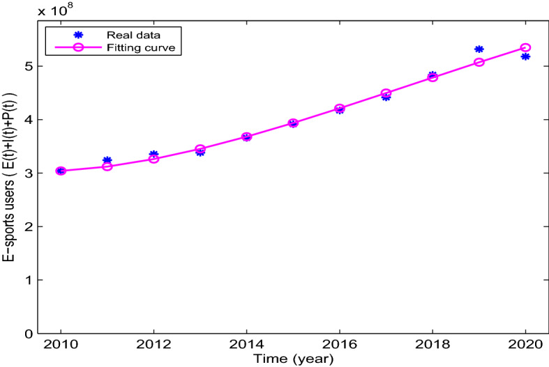
Fitting result to the reported data using model (2)

Table 2.

Estimated parameters for model (2)

Parameters	Descriptions	Values	Sources
$\mu$	Natural death rate	1/77	Assumed
$\alpha$	Contact rate of the addicted users	0.553277	Fitted
$\beta$	Contact rate of the professional users	0.008748	Fitted
${\xi }_1$	Transfer rate from E to I	0.131643	Fitted
${\xi }_2$	Transfer rate from E to P	0.017532	Fitted
$v_1$	Transfer rate from I to P	0.000340	Fitted
$v_2$	Percentage of people who temporarily quit in I	0.097332	Fitted
$v_3$	Percentage of people who quit permanently in I	0.040456	Fitted
$w_1$	Percentage of people who temporarily quit in P	0.002685	Fitted
$w_2$	Percentage of people who quit permanently in P	0.220441	Fitted
${\delta }_1$	Recurrence rate	0.252144	Fitted
${\delta }_2$	Percentage of people who quit permanently in $Q_1$	0.130325	Fitted

Stability of Equilibria

By fitting the real data in the previous subsection, $R_0=5.05$ was obtained. Theorem 4.2 tells us that when $R_0>1$, addiction-present equilibrium (APE) is globally asymptotically stable. We assume the initial value $X_0=(1041152500$, 243280000, 30410000, 30410000, 27398750, 27398750), and use ODE45 in MATLAB to simulate the change process of each compartment in the system. The results are shown in Fig. 3.

Fig. 3.

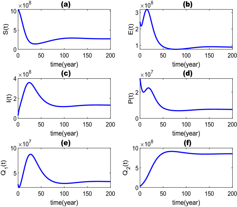
The addiction-present equilibrium $D^{\ast }=(277097542$, 89933450, 133071278, 6869641, 32799019, 860279067) is globally asymptotically stable, and $R_0=5.05>1$

As can be seen from Fig. 3, the addiction-present equilibrium is stable. If we modify the contact rate of addicted users $\alpha$ to 0.05 in Table 1, other parameters and initial values $X_0$ remain unchanged, we can get $R_0=0.46$ through calculation. From theorem 4.1 we can see that the addiction-free equilibrium $D_0$ is globally asymptotically stable when $R_0$ is less than 1. Therefore, we simulate the stability of $D_0$ through MATLAB, and the results are shown in Fig. 4.

Fig. 4.

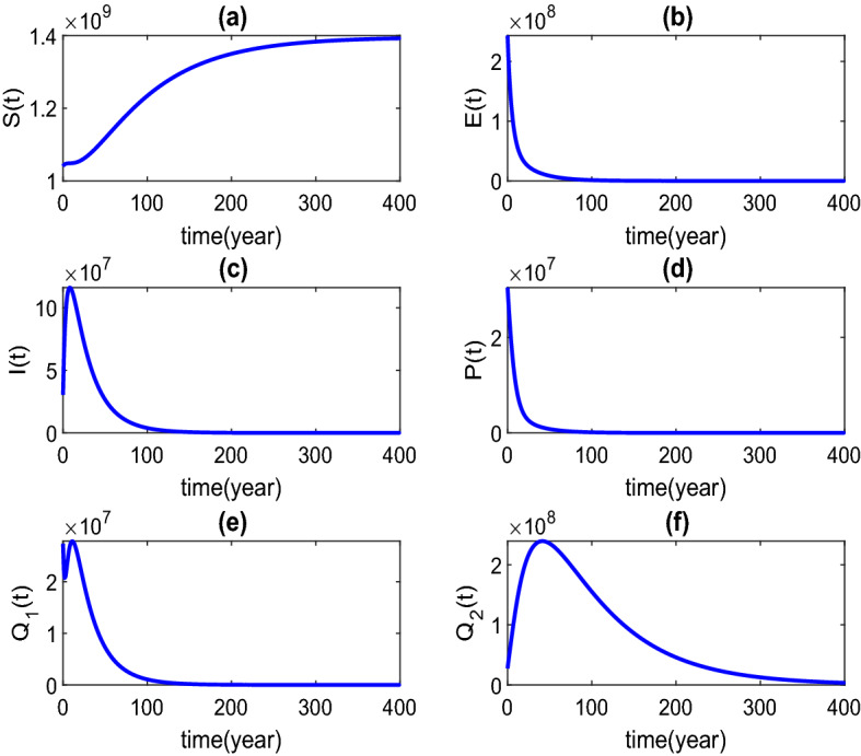
The addiction-free equilibrium $D_0=(1400050000$, 0, 0, 0, 0, 0) is globally asymptotically stable, and $R_0=0.46<1$ when $\alpha =0.05$

Figures 3 and 4 reflect the correctness of the previous theory. From Fig. 3c, we can also see that, as time goes by, the number of addicted people will continue to increase in a short period of time, reaching a peak of 370 million. This is such a serious situation that it is necessary to investigate the issue of controlling game addiction.

The Simulation of Optimal Control

In this section, forward–backward sweep method is used to study the control problem of online game addiction. For more information on this method and its application, see references [2, 8, 9, 15, 20, 27, 28, 30]. In the course of the simulation, we select $A_1=10$, $A_2=10$, $C_1=300000000$, $C_2=1000000$, $C_3=200000000$, and $C_4=35000000$. The values of all model parameters are taken as shown in Table 1. Since the control effect may be affected by many factors during the implementation of the control measures, it is difficult to achieve the ideal 100% effect. So we set the upper limit of the control effect as 0.8. The time of the whole control process is set at 30 years.

In the process of exploring the optimal control strategy, we design the following scenarios to analyze the various combination strategies. Since in the real world, multiple controls are often implemented simultaneously, we will not consider the single control scenario here.

Scenario 1: Coupled control strategies

Strategy A: Isolation$+$Media coverage ($u_1,u_2$).

Strategy B: Isolation$+$Treatment ($u_1,u_3$).

Strategy C: Isolation$+$Family care ($u_1,u_4$).

Strategy D: Media coverage$+$Treatment ($u_2,u_3$).

Strategy E: Media coverage$+$Family care ($u_2,u_4$).

Strategy F: Treatment$+$Family care ($u_3,u_4$).

Scenario 2: Threefold control strategies

Strategy G: Isolation$+$Media coverage$+$Treatment ($u_1,u_2,u_3$).

Strategy H: Isolation$+$Media coverage$+$Family care ($u_1,u_2,u_4$).

Strategy I: Isolation$+$Treatment$+$Family care ($u_1,u_3,u_4$).

Strategy J: Media coverage$+$Treatment$+$Family care ($u_2,u_3,u_4$).

Scenario 3: Fourfold control strategies

Strategy K: Isolation$+$Media coverage$+$Treatment$+$Family care ($u_1,u_2,u_3,u_4$).

Figure 5 shows the changes in the number of exposed and infected people in each strategy under scenario 1. Figure 6 shows the strength of the control variables in each strategy under scenario 1. From Fig. 5, we can see that in strategy A-F under scenario 1, the number of exposed and infected persons in strategy B is the least, and the corresponding control intensity is shown in Fig. 6(B). Control variables $u_1$ and $u_3$ maintain a maximum control intensity of 0.8 at the beginning and continue until 2038 and 2042, respectively, and then gradually decrease to 0.

Fig. 5.

The number of a exposed individuals E(t) and b infected individuals I(t) corresponding to various strategies in scenario 1

Fig. 6.

Optimal control strategies with two interventions (Scenario 1)

The changes in the number of exposed and infected people in each strategy under scenario 2 are shown in Fig. 7. The control strength of each strategy in scenario 2 is shown in Fig. 8. From Fig. 7a, b, we can see that the number of exposed and infected people in strategy G and strategy I is about the same, and is less than that in other strategies.

Fig. 7.

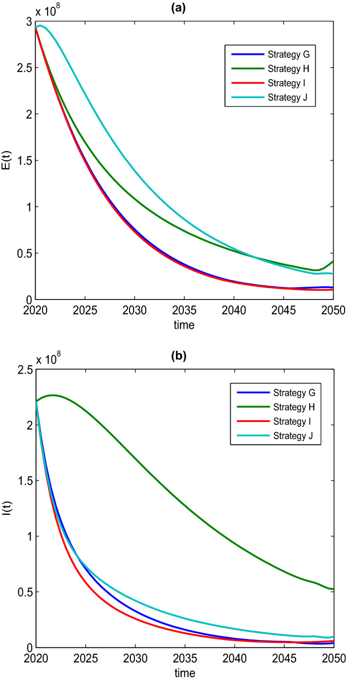
The number of a exposed individuals E(t) and b infected individuals I(t) corresponding to various strategies in scenario 2

Fig. 8.

Optimal control strategies with three interventions (Scenario 2)

In strategy G, the control variables $u_1$ and $u_3$ need to be maintained at the maximum strength of 0.8 at the beginning and continue until 2038 and 2042, respectively, then gradually decrease to 0. The control variable $u_2$ should be kept at 0 at the beginning, gradually increase by 0.8 in 2046, and decrease to 0 in 2049. In strategy I, $u_1$, $u_3$, and $u_4$ all need to be maintained at their maximum strength of 0.8 at the beginning and continue until 2037, 2040, and 2026, respectively, and then gradually decrease to 0.

The changes in the number of exposed and infected people under strategy K and without control are shown in Fig. 9. The control forces in strategy K are shown in Fig. 10. As can be seen from Fig. 9, under strategy K, the number of exposed people and infected people will decrease sharply compared with that without control. These good results are exactly what we want.

Fig. 9.

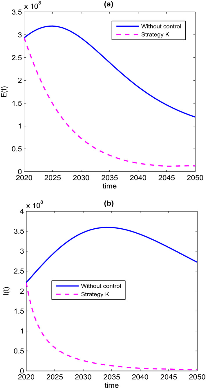
The number of a exposed individuals E(t) and b infected individuals I(t) corresponding to the optimal control strategies in scenario 3

Fig. 10.

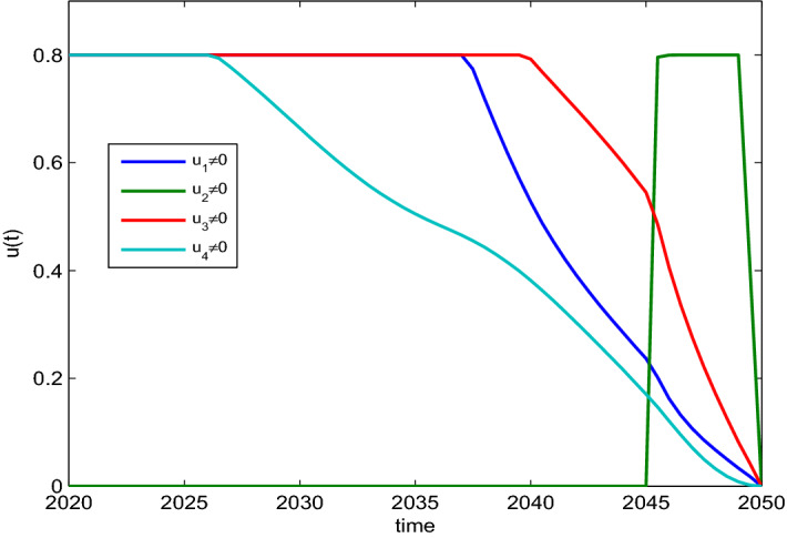
Optimal control strategies with four interventions (Scenario 3)

We found that there are some good controls in all three scenarios, but it was not easy to distinguish them graphically. Therefore, we need to further examine these strategies in terms of specific data indicators. The total infectious individuals (TI) during the control process is defined as follows.

$$\begin{array}{c}\hfill TI={\int }_0^{t_f}\left[(1-u_1(t)),\alpha ,\frac{S(t)I(t)}{N},+,\beta ,\frac{S(t)P(t)}{N}\right]dt.\end{array}$$

The definition expression of the total averted cases (TA) of strategy A is as follows

$$\begin{array}{c}\hfill TA(A)=TI(0)-TI(A),\end{array}$$

where TI(0) denotes the infected users of without control, TI(A) denotes the infected users of strategy A.

From the IAR data in the last column of Table 3, it can be seen that the implementation of strategy K enables more people to avoid infection. Therefore, from this perspective, strategy K is the optimal control strategy we are looking for. Therefore, we suggest that the four control measures should be implemented simultaneously, as shown in Fig. 10, so as to minimize the number of infections.

Table 3.

Comparison of different strategies

Strategy	Total infectious individuals (TI)	Total averted infectious individuals (TA)	Infection averted ratio (IAR) (%)
Without control	957415707	–	–
Strategy A	317432872	639982835	66.8448
Strategy B	70587639	886828068	92.6273
Strategy C	223665375	733750332	76.6386
Strategy D	341337640	616078067	64.3480
Strategy E	858030717	99384990	10.3805
Strategy F	300099591	657316116	68.6552
Strategy G	68720573	888695134	92.8223
Strategy H	223180568	734235139	76.6893
Strategy I	63435930	893979777	93.3743
Strategy J	299216465	658199242	68.7475
Strategy K	61277926	896137781	93.5997

It is worth noting that by comparing the results of strategy G and strategy K, we can conclude that if we increase the continuous family care for the incomplete recovered population, this measure can prevent more people from becoming addicted to the game.

Conclusion

In today’s world, the problem of online game addiction is becoming more and more serious, and it has also attracted the attention of many countries. Many game addicts have an important stage of temporary withdrawal in the process of quitting the game, and they may have a certain possibility of relapse and become addicts again. Based on these considerations, a new mathematical model of online game addiction was established in this paper.

First, we analyzed the basic properties of the model. By means of the next generation matrix, the basic reproduction number with important biological significance was obtained. By constructing appropriate Lyapunov functions, the global asymptotic stability of addiction-free equilibrium and addiction-present equilibrium were proved, respectively.

In the process of numerical simulation, we first collected data from the China Statistical Yearbook, which includes the number of e-sports users in mainland China from 2010 to 2020. The least squares estimation method was used to estimate the parameters of the model, and the approximation of the basic reproduction number $R_0\approx 5.05$ was obtained. From this result, we can see that the transmission problem of game addiction is very serious. Using the obtained parameters, the stability of the equilibria in the previous theory were verified. Finally, through different combination strategies, we got the minimum number of infections under each strategy, and found the optimal control strategy. The results showed that the four control measures should be implemented simultaneously according to the rule indicated by the optimal control strategy, so as to minimize the addicted people.

This paper provided a framework for analyzing and controlling the spread of game addiction, and the results provided a scientific suggestion for the relevant management departments.

Declarations

Conflict of interest

There are no conflict of interest by the authors.

References

- 1.Amin KP, Griffiths MD, Dsouza DD. Online gaming during the COVID-19 pandemic in India: strategies for work-life balance. Int. J. Ment. Health. Ad. 2022;20(1):296–302. doi: 10.1007/s11469-020-00358-1. [DOI] [PMC free article] [PubMed] [Google Scholar]
- 2.Bonyah E, Gómez-Aguilar JF, Adu A. Stability analysis and optimal control of a fractional human African trypanosomiasis model. Chaos. Soliton. Fract. 2018;117:150–160. doi: 10.1016/j.chaos.2018.10.025. [DOI] [Google Scholar]
- 3.Bonyah E, Khan MA, Okosun KO, Gómez-Aguilar JF. Modelling the effects of heavy alcohol consumption on the transmission dynamics of gonorrhea with optimal control. Math. Biosci. 2019;309:1–11. doi: 10.1016/j.mbs.2018.12.015. [DOI] [PubMed] [Google Scholar]
- 4.Diekmann O, Heesterbeek JAP, Metz JAJ. On the definition and the computation of the basic reproduction ratio in models for infectious diseases in heterogeneous populations. J. Math. Biol. 1990;28(4):365–382. doi: 10.1007/BF00178324. [DOI] [PubMed] [Google Scholar]
- 5.Guo Y, Li T. Optimal control and stability analysis of an online game addiction model with two stages. Math. Method. Appl. Sci. 2020;43(7):4391–4408. [Google Scholar]
- 6.Housebound Italian kids strain network with Fortnite marathon. https://www.bloomberg.com/news/articles/2020-03-12/housebound-italiankids-strain-network-with-fortnite-marathon (2020)
- 7.Javed, J. ESports and gaming industry thriving as video games provide escape from reality during coronavirus pandemic. Retrieved from: https://www.wfaa.com/article/sports/esports-gaming-industry-thriving-as-video-gamesprovide-escape-from-reality-during-coronavirus-pandemic/287-5953d982-d240-4e2b-a2ba-94dd60a8a383 (2020)
- 8.Khan MA, Shah SW, Ullah S, Gómez-Aguilar JF. A dynamical model of asymptomatic carrier Zika virus with optimal control strategies. Nonlinear Anal-Real. 2019;50:144–170. doi: 10.1016/j.nonrwa.2019.04.006. [DOI] [Google Scholar]
- 9.Kheiri H, Jafari M. Fractional optimal control of an HIV/AIDS epidemic model with random testing and contact tracing. J. Appl. Math. Comput. 2019;60(1):387–411. doi: 10.1007/s12190-018-01219-w. [DOI] [Google Scholar]
- 10.King DL, Delfabbro PH, Billieux J, Potenza MN. Problematic online gaming and the COVID-19 pandemic. J. Behav. Addict. 2020;9(2):184–186. doi: 10.1556/2006.2020.00016. [DOI] [PMC free article] [PubMed] [Google Scholar]
- 11.LaSalle, J.P.: The Stability of Dynamical Systems. In: Regional Conference Series in Applied Mathematics. SIAM, Philadelphia (1976)
- 12.Lenhart S, Workman JT. Optimal Control Applied to Biological Models. Cambridge: CRC Press; 2007. [Google Scholar]
- 13.Li J, Jiang H, Mei X, Hu C, Zhang G. Dynamical analysis of rumor spreading model in multi-lingual environment and heterogeneous complex networks. Inform. Sci. 2020;536:391–408. doi: 10.1016/j.ins.2020.05.037. [DOI] [Google Scholar]
- 14.Li T, Guo Y. Stability and optimal control in a mathematical model of online game addiction. Filomat. 2019;33(17):5691–5711. doi: 10.2298/FIL1917691L. [DOI] [Google Scholar]
- 15.Li T, Guo Y. Modeling and optimal control of mutated COVID-19 (Delta strain) with imperfect vaccination. Chaos. Soliton. Fract. 2022;156(3):111825. doi: 10.1016/j.chaos.2022.111825. [DOI] [PMC free article] [PubMed] [Google Scholar]
- 16.Ma MJ, Liu SY, Li J. Does media coverage influence the spread of drug addiction? Commun. Nonlinear. Sci. 2017;50:169–179. doi: 10.1016/j.cnsns.2017.03.002. [DOI] [Google Scholar]
- 17.Ma SH, Huo HF, Xiang H, Jing SL. Global dynamics of a delayed alcoholism model with the effect of health education. Math. Biosci. Eng. 2021;18(1):904–932. doi: 10.3934/mbe.2021048. [DOI] [PubMed] [Google Scholar]
- 18.Ngina P, Mbogo RW, Luboobi LS. HIV drug resistance: insights from mathematical modelling. Appl. Math. Model. 2019;75:141–161. doi: 10.1016/j.apm.2019.04.040. [DOI] [Google Scholar]
- 19.Rahman GU, Agarwal RP, Din Q. Mathematical analysis of giving up smoking model via harmonic mean type incidence rate. Appl. Math. Comput. 2019;354:128–148. [Google Scholar]
- 20.Razzaq OA, Rehman DU, Khan NA, Ahmadian A, Ferrara M. Optimal surveillance mitigation of COVID’19 disease outbreak: fractional order optimal control of compartment model. Results. Phys. 2021;20:103715. doi: 10.1016/j.rinp.2020.103715. [DOI] [PMC free article] [PubMed] [Google Scholar]
- 21.Saunders JB, Hao W, Long J, King DL, Mann K, FauthBuhler M. VGaming disorder: its delineation as an important condition for diagnosis, management, and prevention. J. Behav. Addict. 2017;6:271–279. doi: 10.1556/2006.6.2017.039. [DOI] [PMC free article] [PubMed] [Google Scholar]
- 22.Seok LM. Discovering the leisure characteristics of eSports and exploring the possibilities and limitations of eSports academization through autoethnography on the experience of teaching introduction of eSports. J.Korean Leisure Sci. 2022;13(1):23–33. doi: 10.37408/kjls.2022.13.1.23. [DOI] [Google Scholar]
- 23.Sharomi O, Gumel AB. Curtailing smoking dynamics: a mathematical modeling approach. Appl. Math. Comput. 2008;95:475–499. [Google Scholar]
- 24.The China Statistical Yearbook. http://www.stats.gov.cn/tjsj/ndsj/ (2020)
- 25.The seventh National census of China in 2020. http://www.stats.gov.cn/tjsj/tjgb/rkpcgb/ (2020)
- 26.Tian Y, Ding X. Rumor spreading model with considering debunking behavior in emergencies. Appl. Math. Comput. 2019;363:124599. [Google Scholar]
- 27.Ullah S, Khan MA, Gómez-Aguilar JF. Mathematical formulation of hepatitis B virus with optimal control analysis. Optim. Contr. Appl. Met. 2019;40(3):529–544. doi: 10.1002/oca.2493. [DOI] [Google Scholar]
- 28.Ullah S, Khan MA. Modeling the impact of non-pharmaceutical interventions on the dynamics of novel coronavirus with optimal control analysis with a case study. Chaos. Soliton. Fract. 2020;139:110075. doi: 10.1016/j.chaos.2020.110075. [DOI] [PMC free article] [PubMed] [Google Scholar]
- 29.Wu QY, Chen TZ, Zhong N, Bao JW, Zhao Y, Du J, Zhao M. Changes of internet behavior of adolescents across the period of COVID-19 pandemic in China. Psychol. Health Med. 2021 doi: 10.1080/13548506.2021.2019809. [DOI] [PubMed] [Google Scholar]
- 30.Zhang F, Qiu Z, Huang A, Zhao X. Optimal control and cost-effectiveness analysis of a Huanglongbing model with comprehensive interventions. Appl. Math. Model. 2021;90:719–741. doi: 10.1016/j.apm.2020.09.033. [DOI] [Google Scholar]