

Abstract
Modeling and optimization are essential tasks that arise in the analysis and design of supply chains (SCs). SC models are essential for understanding emergent behavior such as transactions between participants, inherent value of products exchanged, as well as impact of externalities (e.g., policy and climate) and of constraints. Unfortunately, most users of SC models have limited expertise in mathematical optimization, and this hinders the adoption of advanced decision-making tools. In this work, we present ADAM, a web platform that enables the modeling and optimization of SCs. ADAM facilitates modeling by leveraging intuitive and compact graph-based abstractions that allow the user to express dependencies between locations, products, and participants. ADAM model objects serve as repositories of experimental, technology, and socio-economic data; moreover, the graph abstractions facilitate the organization and exchange of models and provides a natural framework for education and outreach. Here, we discuss the graph abstractions and software design principles behind ADAM, its key functional features and workflows, and application examples.
Keywords: Supply chain, Optimization, Graph theory, Web tools
1. Introduction
Multi-product supply chains (SCs) arise in a wide range of industrial applications such as energy infrastructures (e.g., biofuels from biomass and coupled electrical power-natural gas systems) (Mitridati et al., 2020; Dueñas et al., 2015), waste infrastructures (e.g., plastic, livestock, food), and chemical manufacturing (e.g., pharma, petrochemical, semiconductors) (Lima et al., 2016; Barbosa-Póvoa, 2014). Recently, many research works involve the use of SC modeling in the context of so-called food-energy-water (FEW) nexus. Understanding FEW systems is challenging since economic, environmental, and societal impacts are coupled in non-intuitive ways, and because such sectors often span multiple geographical scales (local, regional, national, and global) (Finley and Seiber, 2014). For example, organic waste management (e.g., livestock manure and food waste) is tightly coupled with the energy sector (e.g., biogas), the agricultural sector (e.g., crop production), the chemical sector (e.g., fertilizer production), and the dairy sector (e.g., production of milk and derivatives). This coupling arises at dairy farms, which generate large amounts of organic waste from which one can recover valuable energy and nutrient products through technologies such as anaerobic digestion, granulation, and struvite precipitation.
SC modeling and optimization can help navigate the complexity of FEW systems (Pan et al., 2015). A key defining aspect of the multi-product SCs is the presence of product transformation (i.e., products are transformed to obtain other products). Multi-product SCs typically involve a wide range of participants (stakeholders) such as suppliers and consumers of products, providers of transport, processing, and storage (inventory) services, and other external actors (e.g., policy). This creates a transaction network (a graph) that exhibits complex interconnectivity across products, stakeholders, and spatial (geographical) locations. Specifically in FEW systems, the SC models contain different products and participants (suppliers, consumers, technology pathways, and transportation pathways) that exchange, transform, and transport such products. These models capture how raw products from suppliers are delivered to technologies and transformed by such technologies to obtain intermediate and final products, which are then delivered to other technologies or to consumers. Moreover, with different SC setups, participants can be competitive, strategic, and profit-maximizing entities (Garcia and You, 2015; Papageorgiou, 2009); as such, understanding the emergent behavior of product flows and of their inherent monetary value (prices) in FEW systems is challenging.
Diverse software products have been developed for modeling and analyzing FEW nexus systems. Daher and Mohtar developed FEW Nexus Tool (Daher and Mohtar, 2015), a modeling platform for evaluating scenarios and identifying sustainable resource allocation strategies. This tool considers environmental (e.g., water and energy) and financial aspects of FEW systems and models the interactions between them to compute an overall sustainability index. Martín-Hernández et al. (2021) proposed a web-based, decision-making application that recommends technologies for dairy farms considering farm size, animal type, eutrophication risk, and other factors. Some other tools for integrated modeling of FEW nexus include WHAT-IF, NexSym, and PRIMA (Payet-Burin et al., 2019; Martinez-Hernandez et al., 2017; Kraucunas et al., 2015); these tools place emphasis on water planning, climate change, land use, and other specific applications. Most of these tools incorporate comprehensive datasets and empirical decision-making criteria. Other tools developed in the process systems community use mathematical optimization to facilitate the selection and assessment of processes and operations; an example of such tools is p-graph studio, developed by Bertok et al. (2013), which conducts process-network synthesis in a process graph (p-graph) representation. Ng et al. (2018) developed a web application called BUS for superstructure optimization of biomass-to-fuel processes. As can be seen, most of the software products in the FEW domain automate analytical methods for specific applications instead of general SC modeling.
At the same time, researchers have put lots of efforts in developing SC models, theories, and case studies for the FEW nexus systems. Sampat et al. (2017) recently proposed a modeling abstraction that leverages concepts of graph theory to capture diverse elements and connectivity that arises in these types of SC models. This abstraction has revealed that SCs can be interpreted as coordinated markets in which participants exchange, transform, and transport products to generate economic value (Sampat et al., 2019; Tominac and Zavala, 2020). This provides a natural framework for understanding the impact of policy incentives, to monetize environmental impacts, and to discover the inherent value of products. Moreover, it has been shown that graph modeling abstractions provide interesting insights that explain how revenue flows from consumers to suppliers, technologies, and transportation providers. These abstractions have been used to tackle diverse FEW nexus problems such as recovery of biogas and struvite from livestock waste, understanding the economic impacts of nutrient pollution from dairy farms, promoting landfill diversion of municipal solid waste into recycling technologies, and recovery of nutrients from livestock manure using cyanobacteria (Sampat et al., 2018a; Tominac et al., 2020; Sampat et al., 2018b; 2021; Ma et al., 2021). We also note that many of those developed methods are general and broad enough to be applied in fields outside of FEW systems. In terms of software for SC management, various commercial products exist for conducting business tasks such as demand forecasting and inventory tracking. The U.S. Department of Energy developed MFI (Carpenter et al., 2014) to evaluate energy and material flows across different industrial sectors. Reich-Weiser et al. (2008) proposed a SC tool called SCOPR to assess energy and greenhouse gas metrics in solar energy technologies. Lin et al. (2015) designed a Cyber-GIS-based SC optimization tool for analyzing and optimizing biomass-to-ethanol supply chains in the U.S.
To the best of our knowledge, there is no general open-source SC optimization tool that can help make decisions on technology selection and transport. This gap is surprising, given the widespread availability of models and case studies (particularly in the context of FEW systems) (Abdali et al., 2021; You and Wang, 2011; Sampat et al., 2018a; Hu et al., 2018). Motivated by this, here we present ADAM, which is a web-based platform for the modeling and solution of multi-product SCs. ADAM uses compact graph-based modeling abstractions, which facilitates model implementation by users with limited mathematical optimization expertise (e.g., policy makers and undergraduate students). The availability as a web tool also facilitates access by users that have limited access to computational resources (e.g., computer servers and optimization software needed to run SC models). ADAM incorporates an object-oriented data management system that is directly informed by the graph-based modeling abstraction; here, SC models and data are treated as objects that are built in a modular manner and that are easily exchanged and reused. ADAM is designed to bridge the field of SC optimization with experimental research, technology development, and education in FEW systems and in the broader field of SC management. In this paper we provide a comprehensive review of the design principles of ADAM, including graph-based formulations of SCs and associated data structures. We introduce key features and computational workflows, and a couple of case studies are presented to show the capabilities of ADAM, including an example arising in organic waste management and an example arising in plastic waste recycling.
2. Software design principles
In this section, we introduce the main design principles of ADAM. We introduce the mathematical optimization models that are implemented and how these interact with data structures and visualization tools. We highlight these abstract models are not seen by the user interacting with ADAM; all modeling conducted by the user takes place in a visualization interface. This dramatically reduces the expertise needed by the user and makes the application intuitive to use; for instance, ADAM has been used in the undergraduate course CBE 450: Process Design at the University of Wisconsin-Madison to teach students how to optimize complex SCs.
2.1. Supply chain modeling
The mathematical model framework behind ADAM is the multi-product SC optimization model proposed by Sampat et al. (2017). This model uses a graph representation that is coupled in space (via transportation) and across products (via transformation). In this graph representation, the node set contains geographical locations for suppliers, customers, and technologies. Each node has geographical attributes (latitude and longitude). The set represents the collection of all products (materials) in the system, including raw materials, intermediate products, and final products. The definition of a product is flexible in that it can represent any abstract resource (e.g., materials, energy, labor). The set denotes the collection of all technologies in the system. The set denotes all suppliers and the set represents all consumers. The set of denotes the collection of transport links (graph edges) that move product between nodes. Each supplier, consumer, technology, and transport link have an associated set of data attributes (e.g., cost, capability, location).
Product Balances.
The first set of constraints in the model is product balance constraints. Eq. (1) is a balance for product p at node n, and this balance holds for any arbitrary product in the set and any node in set . The left-hand side contains a supply term sn,p, a total inflow term , and a term to represent the net generation of product p at node n from technologies. The net generation term can be either positive (product is produced) negative (product is consumed) or zero (product is neither produced nor consumed). The right part of the equation contains a demand term dn,p and a total outflow term .
Eq. (2) captures product transformations through technologies. The generation of product p at node n through technology t is calculated using the generation term of the reference product for the technology , and the relationship between the yield factors γt,p. We note the γt,p is defined to ensure that transformation can only occur from feedstock to product, not the reverse. The reference product typically denotes the main feedstock of the technology and is used for quantifying processing capacity and costs. We use to represent the reference product of technology t.
| (1) |
| (2) |
Capacity Constraints.
We use (3)–(5) to capture the capacities for supply, demand, and generation. In these constraints, we use sn,p, to represent the lower and upper bound for supply sn,p, dn,p, to represent the lower and upper bound for demand dn,p, and to represent the lower and upper bound of processing capacity of technology t.
The binary variable yn,t is used to indicate whether technology t is installed at node n. Specifically, if yn,t = 1, then the generation term is bounded by the capacity ranges of technology t; if yn,t = 0, then the generation term is zero, meaning there is no product transformation. Sometimes, before solving the model, we know some nodes already have technologies installed. In that case, the corresponding binary variable yn,t can be prefixed. We note that if all the binary variables yn,t are fixed, the model reduces to a linear programming problem, where the model is purely used for analyzing the systematic performance of installed technologies. Under this condition, the system behaves like a coordinated market (Sampat et al., 2019) and we refer to this special case as a supply chain management model, whereas others as a supply chain design model when there is at least one unfixed binary variable(s).
| (3) |
| (4) |
| (5) |
Modelers are occasionally interested in the outcomes of a SC acting under fixed supply or demand, regardless of the economic feasibility. In this supply chain design - fixed scenario, we allow nonzero values of the lower bound parameters sn,p, dn,p, and ξt in (3)–(5). We observe that, from a theoretical perspective, negative profits may be observed when these parameters have any nonzero value, but that the capability to “force” a solution in ADAM is useful at times. Tominac and Zavala provide the theoretical reasoning showing how these lower bounding values are linked to profit (Tominac and Zavala, 2020).
Objective Function.
The economic metrics considered in the SC model include technology investment cost, technology operational cost, supply cost, transportation cost, and value of demand served. The annualized investment cost of the technologies is captured by Eq. (6), where r is interest rate, N is the expected life of technologies, Kinv,t is the fixed part of investment cost for technology t, and Binv,t is the proportional part of investment cost for technology t. We note the binary variables are only defined for those that are not prefixed (if some technologies are pre-installed and the corresponding binary variables are prefixed then they are excluded in the investment calculation). Eq. (7) is used to compute the operational cost of technologies, where Kop,t is the fixed part of operational cost for technology t, and Bop,t is the proportional part of operational cost for technology t. We can observe that if a technology t is not installed at node n, then yn,t = 0, meaning according to (5), then the corresponding investment and operational costs are zero as well. Eq. (8) is used to compute the transportation cost, where Dn,n′ is the transportation distance between node n and n′, and is the transportation cost of product p per unit flow per unit distance. The transportation distance between nodes can be estimated by longitude and latitude (Ballou, 1998).
We use (9) and (10) to calculate the supply cost and revenue from demand served. In these equations, represents the per unit supply bid (which ultimately influences the resulting market price) of product p at node n, and represents the per unit demand bid for product p at node n.
| (6) |
| (7) |
| (8) |
| (9) |
| (10) |
The objective function of the SC model is to maximize the total welfare, defined in (11). The welfare is a composite metric that fuses all economic metrics defined previously. Maximizing the welfare aims to maximize the value of the demand served while minimizing costs associated with supply, transport, and technology operation/investment.
| (11) |
The SC model can be used for solving management and design problems. In a management problem, all technologies have been specified and thus the investment cost Cinv is a constant and can be eliminated. In an SC design problem, a subset of the technologies are selected in a way that they minimize the investment cost Cinv.
The SC model can be interpreted as a market clearing model in which participants transact and transform products to maximize welfare. Recent work has shown that maximizing this objective is equivalent to maximizing the total profit of all participants. Here, the dual variable of the product balance (1) (which we denote as πn,p) can be interpreted as clearing prices that capture the inherent value of product p at location n. The clearing prices provide important insights into how suppliers, technologies, and transportation should be remunerated for their services and into how consumers should be charged. In-depth analysis of price behaviors under coordination is provided by Tominac and Zavala, who identify price bounding relationships emerging from stakeholder bids (Tominac and Zavala, 2020).
Model Output
The solution of the SC management problem delivers optimal allocations for all participants along with dual variables representing the product prices at each graph node; these dual variables are referred to as nodal prices for this reason. Primal and dual variables together provide information about physical product flows and transformations, as well the prices of products and services in a supply chain.
2.2. Graph-based abstraction
The definition of the model defined in Section 2.1 is performed in a couple of subsequent stages. In the first stage, we define the set of nodes , set of products , and the set of technologies . In the second stage, we define data attributes for suppliers, consumers, technologies, and transport links. For example, for a given technology, we need to specify technology type, location, cost (operation and installation), capacity, and yield factors.
The SC modeling framework leverages concepts of graph theory to construct the model; here, we use a process graph (p-graph) to specify technology pathways (and product interconnectivity) and a geographical graph (g-graph) to specify locations of technologies, suppliers, and consumers (and geographical interconnectivity).
Process Graph (p-Graph).
A p-graph is a directed graph that is used to represent a process (pathway) structure; it was originally proposed by Friedler et al. (1992, 1993). Here, pathways are interpreted as sequences of processing steps that transform products into other products. P-graphs have been widely used in process synthesis and superstructure optimization (Varbanov et al., 2017; Wu et al., 2016; Voll et al., 2013).
A p-graph is represented by the node-edge set pair , where is the set of nodes (vertices) and is the set of edges. The set can be further partitioned into disjoint sets, denoted as and , such that and . The vertices in (denoted M vertices) represent all possible products involved in a process, while the vertices in (denoted T vertices) represent all possible steps in a process. For simplicity, we use the following notation to represent elements in the sets, where mi and ti represent some product and step in the process. Furthermore, a step ti can be further represented by a tuple , where is the set of feedstocks of the step, and is the set of products of the step; clearly, we have . The step ti is capable of transforming products in to products in according to transformation rules.
| (12) |
| (13) |
The set in the p-graph can be partitioned into disjoint sets, denoted as and :
| (14) |
where
| (15) |
| (16) |
The set includes edges that go from one feedstock of some technology to that technology, and the set includes edges that go from some technology to one of its products. An edge can only exist if the corresponding transformation is physically realizable. Therefore, a p-graph always starts and ends on at least one M vertex. Vertices with no input edges represent raw products for the system, vertices with no output edges represent final products, and vertices with both input and output edges represent intermediate products. This representation forms a product hierarchy that moves from raw products to intermediate and to final products. There are no disconnected vertices in a p-graph; every vertex must be connected to at least one other vertex. Moreover, every pair of adjacent vertices , must be of different categories (if v1 is a M vertex then v2 is a T vertex).
An example of a simple p-graph is given below in Fig. 1, where and . The graph represents a process structure where raw material m1 can be converted to m2 and m3 through technology t1 = ({m1}, {m2, m3}), and then intermediate products m3 can be further transformed to m4 by technology t2 = ({m3}, {m4}). In this example, vertices in set are displayed as circles and vertices in set are displayed as rectangles. Edges in set are shown in black, and edges in set are shown in blue.
Fig. 1.

Structure of a representative p-graph.
We note that each p-graph defines a process structure and thus additional data needs to be attached to T vertices and edges. Each T vertex is associated with information of processing capacity (upper bound and lower bound ξt), investment cost (fixed part Binv,t and proportional part Kinv,t), and operational cost (fixed part Bop,t, and proportional part Kinv,t). These data fully specify constraints (5)–(7).
Each arbitrary edge contains data on the corresponding transformation coefficient γe. Specifically, if , then we have γe = γt,p where t = v1 and p = v2; otherwise, if , then γe = γt,p where t = v2 and p = v1. Furthermore, the transformation coefficient of the reference product of technology t in a p-graph is defined in (17). By default, we select the main feedstock of step t; thus, the data in set fully specifies constraints (2).
| (17) |
In Fig. 1, we observe the transformation relationships among products on the edges. Every unit of product m1 can be converted to 0.2 units of m2 and 0.8 units of m3 through technology t1, as indicated in red above each edge. The negative sign of transformation coefficient of m1 represents that it is consumed in the technology. Then, for every unit of m3, it can be further transformed to m4 through technology t2. For technology t1, its operating capacity is 100–1000 units of m1 per year, with an investment cost of 1 million USD and operational cost of 100 USD per unit of m1. Similarly, for technology t2, its operating capacity is 80–800 units of m3 per year, with an investment cost of 0.5 million USD and operational cost of 40 USD per unit of m3.
A p-graph can be used to obtain the entire technology set and product set and it can help model builders to define all possible transformation pathways in an SC. Fig. 2 provides an example of a p-graph for a livestock waste SC study reported in Sampat et al. (2019). Here, the livestock waste is separated into solid and liquid fractions; the solid fraction enters a granulation step, and the liquid fraction is processed by a struvite recovery technology.
Fig. 2.

Example p-graph arising in livestock waste processing.
Geographical Graph (g-graph)
A g-graph is a directed graph that is used to express geographical interconnections between participants in the SC. A g-graph is represented as , where is the set of vertices and is the set of directed edges. The set can be further partitioned into four disjoint sets, denoted as , , , and , i.e.,
| (18) |
| (19) |
The vertex sets , , , and represent suppliers, consumers, existing technologies, and candidate technologies in the system. We use si, di, tpi, and tci to represent elements in these sets. Each node in a vertex set has associated attributes; each supply node is defined with corresponding supply product , a supply capacity , and a supply bid . Similarly, each demand node di is defined with corresponding demand product , a demand capacity , and a demand bid . As for the technology provider nodes tpi, each is specified by the installed technology and processing capacity . And each technology candidate tci is specified by the technology that can be installed, .
The set of edges in a g-graph is determined when all vertices are defined with necessary data. Specifically, an element in set can be denoted as e = (v1, v2, p) and it represents a valid transportation route of product p from vertex v1 to v2. The set in a g-graph can be further partitioned into four disjoint sets, denoted as , , , and , i,e.,
| (20) |
where
| (21) |
| (22) |
| (23) |
| (24) |
These conditions imply that product p can be directly transported from v1 to v2 if v1 supplies p and v2 demands p; v1 supplies p and v2 has (or can install) some technology that takes p as feedstock; v1 has (or can install) some technology that generates p as product and v2 demands p; v1 has (or can install) some technology that generates p as product, and v2 has (or can install) some technology that takes p as feedstock.
Each edge e = (v1, v2, p) is associated with the transportation cost of moving one unit of product p along this edge, denoted as Ce. Normally, Ce can be computed as a linear function of the distance between v1 and , i.e., , where Ctrans,p is the unit transportation cost of product p. The distance can be calculated if the geographical coordinates of the vertices are specified, and the unit transportation cost can be treated as an attribute of the product transported.
In Fig. 3, we give an example of a small g-graph, containing 2 suppliers (yellow), 2 consumers (green), 1 technology provider (blue), and 1 technology candidate (red). Both suppliers offer product m1 but with different capacities and bids. The technology provider offers technology t1, which can convert m1 into m2 and m3. The technology candidate offers t2, which can convert m3 into m4. One consumer can consume product m2 with a capacity of 200 kg per day at a bid of 8 USD per kg of m2. Another consumer can consume product m4 with a capacity of 320 kg per day at a bid of 4 USD per kg of m4. Product m1 can be transported from s1 or s2 to tp1, where technology t1 uses m1 as feedstock. Product m2 can be generated from t1 in tp1 and consumed by d1. Product m3 can be generated from t1 in tp1 and then used as a (potential) feedstock of t2 in tc1. Finally, product m4 can potentially be generated by t2 in tc1 and then consumed by d2. Each edge in the g-graph is assigned with the corresponding transportation cost.
Fig. 3.

Example of g-graph.
For a g-graph, it can completely replace the node set in the mathematical formulation and define the geographical property in a simpler way. We note that a g-graph and p-graph are closely tied due to shared product and technology elements. Specifically, the product attribute of vertices in of a g-graph points to elements in of a p-graph, and the technology attribute of vertices in points to elements in of a p-graph.
2.3. Data structures
The graph-based modeling abstraction facilitates the development of an object-oriented framework to specify and manage SC model data. The overall data structure is shown in Fig. 4. Each graph model object includes a p-graph and a g-graph model object.
Fig. 4.

Overall data structure implemented in ADAM.
A p-graph data object is defined by its vertices and edges, where the vertices include the set of products and the set of technologies, and the edges include the set of all transformation relationships. Specific products, technologies, and transformation relationships are treated as objects. Each of these objects has corresponding attributes that need to be specified when defining the p-graph; for example, we need to specify capacity and cost data when defining a technology.
A g-graph data object is defined by its vertices, and edges can then be automatically generated based on (21)–(24). Vertices in a g-graph include the set of suppliers, consumers, and technologies. Demand and supply vertices require an attribute of product that is supplied or consumed, which points to an element in the product set in the p-graph. Similarly, technologies require a technology attribute to specify if this is installed or can be installed; this attribute points to an element in the technology set in the p-graph. This proposed data structure forms the foundation of data storage and management systems in ADAM.
3. Software implementation
3.1. Product and technology database
From the proposed data structure, products (materials) and technologies are fundamental elements in the SC graphs. Specifically, vertices in a p-graph exactly represent products and technologies, while vertices in a g-graph are built upon products and technologies in the p-graph. Therefore, identifying valid products and technologies is necessary prior to building the SC model.
Models implemented by users typically have overlap in the types of products and technologies used. For example, in the context of manure management, common products include manure, biogas, and digestate, while common technologies include anaerobic digestion and solid-liquid separation. As such, modeling efforts can be largely reduced by leveraging existing databases of products and technologies. Inspired by this, we implemented a product and technology database in ADAM. In addition to the attributes displayed in Fig. 4, some additional auxiliary attributes (metadata) are defined in the database, such as product descriptions and engineering units. Transformation relationships are stored in an implicit database that connects products and technologies.
An illustration of the database is provided in Fig. 5. The product/technology database records information and parameters for each product/technology, while the transformation database tabulates the coefficient of products in technologies. For instance, in the transformation database in Fig. 5, item 1 indicates the transformation coefficient of product m1 in t1 is − 1, meaning that m1 is the main feedstock (and reference product) of t1. On the other hand, item 2 in the transformation database indicates the transformation coefficient of product m2 in t1 is 0.5, meaning that m2 is one product of technology t1.
Fig. 5.

Sketch of product (material) and technology database in ADAM.
The ADAM database contains a public component and a private component. The public database is maintained by admin users (immutable to other users) and accessible to all users; this database is used to record commonly used products and technologies and has been carefully evaluated based on literature reports. Apart from the public database, each user keeps a private database that is not accessible by any other user. Within its private database, each user can define and save custom products and technologies for their own use. When building a graph-based SC model, users have access to both public and private databases (Figure S3).
3.2. Graph construction
The database defines all possible technologies, products, and transformation pathways that can be used to build the SC model. Users are thus not required to provide a complete p-graph every time a SC model is being built. Instead, ADAM directly pulls out corresponding products, technologies, and pathway data.
ADAM provides an interactive visualization interface for users to build p-graphs and g-graphs. The interface employs an open-source mapping system (OpenStreetMap Haklay and Weber, 2008) where users can place any type of geographical vertices. For each vertex, in addition to the attributes defined previously, ADAM further requires geographical coordinates for transportation distance estimation (Goetschalckx, 2011). In Figure S1, we show an example of a g-graph (nodes only) in the ADAM interface.
To reduce complexity, the g-graph construction is decomposed into three steps: supply specification, demand specification, and technology specification. Based on the specific application, users are required to identify the products in the SC. Then, for the first two steps in ADAM, users must place them as suppliers and consumers and input required attributes. ADAM can automatically identify feasible technology pathways from the database (algorithm 1 in supplementary information). Among those feasible technologies, users will specify the ones of interest in the third step and place them as technology providers or technology candidates. As users construct the g-graph by adding different materials and technologies into the SC, the p-graph is populated incrementally and automatically by the ADAM backend (Fig. 6). To facilitate graph construction for new applications, product and technology creation is included as a part of the construction procedure. Users are allowed to add new products and technologies to their private databases on-the-fly in graph construction. Users are able to pre-define products and technologies through the product and technology databases without having to build a SC.
Fig. 6.

Illustration of g-graph construction procedure.
After all vertices in a g-graph are defined, the edges (which represent all possible transportation routes) can be generated automatically by ADAM based on rules (21)–(24). Figure S2 shows the complete g-graph for the example shown in Figure S1.
3.3. Model management
An SC model is fully defined once its associated p-graph and g-graph are defined. A specific SC model is stored as a g-graph only and the corresponding data contain all g-graph components and their attributes. The p-graph of that SC model can be easily constructed by extracting products and technologies from g-graph vertices attributes. Like products and technologies, ADAM provides auxiliary attributes (metadata) to help users manage their model objects (e.g., model name and description).
ADAM provides methods to manipulate SC model objects. For instance, a specific SC model (along with its associated p-graph and g-graph) can be easily duplicated. This allows users to conduct parametric studies (sensitivity analysis) by duplicating a baseline model and modifying specific components in the associated graphs. This capability can be used to extend an existing baseline model (e.g., by adding products and technologies to an existing model). Users are also allowed to merge SC models; in this merging procedure ADAM will automatically take the union of the corresponding g-graphs and p-graphs. This highlights how the graph abstraction can be used to build complex models in a modular manner.
The SC models are classified as public and private; public models (case studies) use products and technologies from the public database and have been verified. Any user can view and make a copy of public models; once copied, users can modify data. This feature provides a modeling template for new users and facilitates learning. Users can build private models by using materials and technologies from public and private databases. A private model can only be accessed and modified by its owner. Admin users do not have permission to make a copy of a private model and then publish it as a case study unless the p-graph uses the public database only (Fig. 7). This structure is designed to maintain privacy of databases (e.g., that contain proprietary information).
Fig. 7.

Model management strategy implemented in ADAM.
3.4. Software architecture
The current version of ADAM can be accessed at (http://ADAM.che.wisc.edu:8000) and is implemented as a web tool to provide easy access to a wide variety of users. This application is developed using a high-level Python-based (Python 3.7) website development framework, Django (version 2.0.0+). With Django, ADAM can directly communicate with database software and render HTML templates. On the back-end, the database software used by default is MySQL (8.0.0+), but PostgreSQL (12.0+) has been tested and is compatible. The optimization models are implemented in JuMP, a Julia (1.0.0+) package for algebraic modeling. The optimization solver used is Clp (for linear programming) and Cbc (for mixed-integer linear programming), which are open-source solvers for linear and mixed-integer linear programming.
On the front-end, we use Bootstrap (4.3.1+) and JQuery (1.12.1+) for enhancing the functionality of webpage styling and interactivity. Leaflet (1.6.0+) and related additional plugins are used for implementing the geographical mapping system. Other auxiliary packages include AlertifyJS, Draw2D, and Ionicons; Fig. 8 summarizes the packages that support ADAM.
Fig. 8.

Software packages used in ADAM.
4. Computational workflows
4.1. Basic setup
The current version of ADAM has the following elements in the navigation bar: HOME, ABOUT, TUTORIAL, DASHBOARD, and CONTACT. The HOME page of ADAM is shown in Fig. 9. It consists of a simplified SC model to get users familiar with the general functionality of ADAM. The simplified model only considers predefined materials and technologies with price data only. The ABOUT page redirects the user to another page which contains extensive documentation on the case studies in ADAM as well as more in-depth tutorials on building models. First-time users are encouraged to go over the TUTORIAL section before registration and building up their own models. Two example models with documentations are included in TUTORIAL. Each example contains eight steps, where the first two steps explain model input and output data, and the remaining six are for model construction. The model construction contains steps for the specifications of model type, supply data, demand data, technology data, transportation data, and model execution (Fig. 10).
Fig. 9.

ADAM homepage.
Fig. 10.

Steps in tutorial examples.
The first example is a SC management model about using livestock waste to generate electricity. The data in this example are predefined and the model is pre-solved so that first-time users don’t have to wait for the model to be solved in the learning process. The second example is a supply chain design model, where an additional technology candidate is added. This model allows users to partially modify some of the input data, such as the locations of g-graph vertices, the price and capacity of supplies and demands, etc. The model is solved immediately after users click the run model button, and users will then be redirected to a separate page to view results sent back from the ADAM back-end server. Once users become familiar with the general steps in model building, they can go to the DASHBOARD and then register for an ADAM account. Registered users have access to the dashboard and can enter the material and technology database system, case studies published, user model management system, and an embedded visualization tool.
4.2. Model building
Users can choose to build a model from an existing case study or from a blank template. Published case studies provide all datasets and comprehensive documentation (from which users can obtain background information on the model and the detailed reasoning behind setting p-graph, g-graphs, and corresponding data). Once a case study is published, users have the freedom to conduct sensitivity analysis studies (i.e., modify and resolve the model and then compare with public results). For more advanced users who wish to build up customized SC models, ADAM provides an alternative model building method where users can create a new, blank model. In many situations customized models involve adding new products and technologies that are not available in the databases; users can choose to enter all necessary materials and technologies into the database system, either before building the model or on-the-fly during the model construction steps.
The model building procedure is divided into six steps, which are the same as the tutorial examples. The first step is to specify the model type, where two options are available: SC management and SC design. A management model can only use technology providers to achieve material transformation, while a design model allows new technologies to be installed (they can be added as technology candidates). In steps 2–4, supply, demand, and technology data are required. ADAM provides several options for data input, including inputting data manually, uploading CSV data files, and loading data from another model. For the manual option, ADAM provides an empty form with fields of geographical locations and g-graph vertex attributes for users to fill. For the data uploading option, ADAM provides a template CSV file where users can put their data, and with that format, ADAM can compile the file into graph components. When loading data from another model, ADAM directly copy the specified data category (e.g., suppliers) from the selected model. In Fig. 11(a) and (b), we show screenshots of supply data specification by manual input and data upload, respectively. In each step, ADAM conducts a data validity check to make sure all input data are of the correct format and valid for use (e.g., supply price and capacity should be float numbers). In step 5, transportation routes will be generated automatically by ADAM and the model is ready for execution.
Fig. 11.
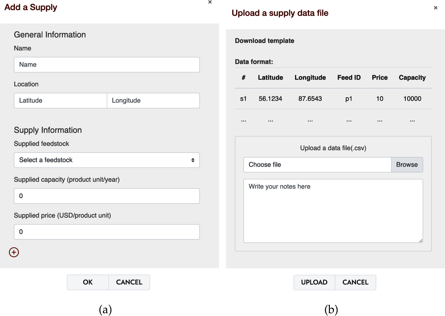
Supply data specification in ADAM (a) manual input (b) data upload.
4.3. Model solving and visualization
Once all data components are correctly set, the “Run” task in step 6 will be activated and users can execute the model. A couple of e-mails will be sent to users separately when the model starts to run and finishes solving. Once the model solution procedure ends, ADAM reports the status of the model of either completed or error (which usually arises from unbounded or infeasible model due to improper input data). In the former case, ADAM reports the systematic performance of the SC, including the overall social welfare, total revenue, supply cost, transportation cost, technology investment cost, and technology operational cost. The detailed model results will be available in the ADAM visualization tool, where users can view the optimal SC setup, such as optimal technology placement and processing capacity, supply and demand amount, and transportation routes. For the SC management model, the clearing price of each product is retrieved from the solver and plotted as a colored contour map. An example of result visualization of a simple model in ADAM is given in Fig. 12, where the optimal transportation routes of three products are plotted as directed lines with different colors, and the price map for cow manure is displayed. Other results can be visualized by clicking the corresponding g-graph components.
Fig. 12.

Visualization of model results.
5. Application examples
In this section, we demonstrate the modeling capabilities of ADAM using a couple of application examples on waste management. Here, we discuss how to construct p-graphs and g-graphs and navigate model results. The case studies can be found in ADAM documentation.
5.1. Biogas production
Livestock waste can be used for producing biogas through anaerobic digestion (AD) technology. The generated biogas is commonly used for electricity generation or for heating purposes. However, AD systems in the US are constantly facing economic barriers, mainly due to high uncertainty in investment and operation costs, and relatively low market value of the recovered products. Therefore, to motivate the use of renewable energy, the US has been providing an incentive called Renewable Energy Certificates (RECs). Under this scheme, every unit (MWh) of renewable electricity generated receives a REC, and the producer of renewable energy can then sell the RECs either in a compliance market or a voluntary market Sampat et al. (2018b).
In this example, we examine the impact of REC value on a dairy manure SC and the installation of AD systems in Upper Rock River Watershed, Wisconsin, United States. The p-graph and g-graph of the relevant case study are shown in Fig. 13(a) and (b), respectively. Cow manure is collected from concentrated animal feeding operations (CAFOs, large farms consisting of 1000 or more animal units) and can be used for electricity generation via AD. For one metric tonne of cow manure, 31.2 kWh of electricity and 0.98 metric tonne of by-product, digestate, will be generated. In addition, a hypothetical product is produced along with renewable energy, i.e., 0.03 unit of RECs (since 1 MWh of renewable electricity equals 1 REC). We note that this is a common modeling technique that can be applied to capture and assign value to additional benefits or impacts of interest of a process, such as carbon emissions and water consumption. The technology investment and operation cost data are collected from various resources. In the g-graph, 22 CAFOs in the study region are included. Each CAFO acts as a supply, technology candidate, and demand entity simultaneously. The supply amount of cow manure is estimated by the farm size. The CAFOs can consume electricity onsite with a market value of 0.08 USD/kWh and use digestate in land application. The hypothetical product, RECs, are assumed to be sold locally with some specified economic incentive.
Fig. 13.

p-graph (a) and g-graph (b) for biogas production example.
The SC design for REC incentive values of 0 and 100 USD/MWh are shown in Fig. 14(a) and (b), respectively. We can observe that, without a government incentive, electricity recovery is not economically viable, resulting in no technology installment. All farms act as suppliers and consumers of manure, indicating that manure is collected and directly utilized in land applications only. When the value of RECs is increased to 100 USD/MWh, the energy recovery technology becomes economically attractive; all manure in the study region is used for electricity generation. We observe that most CAFOs (18 out of 22) install the technology, whereas technology investment is not considered in the remaining farms due to transportation logistics (i.e., they have CAFOs nearby and transporting manure is cheaper than investing in a new technology).
Fig. 14.

Results for biogas production example with different REC value (a) 0 USD/MWh (b) 100 USD/MWh.
5.2. Plastic waste recycling
The production of plastic products and associated plastic waste have grown at an extraordinary rate. Traditionally, plastic waste either accumulates in landfills since it rarely degrades under natural conditions or ends up in incinerators to recover energy in the form of electricity or steam. Recently, various pathways to extract more valuable products from plastic waste via recycling technologies have been investigated. This enables the substitution of virgin resin with recycled resin that exhibits comparable properties and avoiding economic and environmental burdens related to extraction and production of virgin resin.
In this example, we illustrate a case study for the plastic waste SC of polyethylene terephthalate (PET) bottles in the State of Wisconsin. The p-graph of the SC is shown in Fig. 15(a), where PET pellets are used to produce PET preforms to be blown/molded to make PET bottles; those bottles are then filled with beverages and sold to customers. Once the customer consumes the beverage, the discarded bottles are collected and directed to material recovery facilities (MRFs). After the sorting step at MRFs, empty bottles are directed to a waste handling facility or transformation technology at convenience. In this case study, we considered three end-of-life scenarios for empty bottles; they can be (i) discarded to a landfill, (ii) incinerated to produce electricity through waste-to-energy-technology (WtE), or (iii) mechanically recycled into rPET (recycled PET) pellets. For one metric tonne of PET waste, 2076.7 kWh of electricity can be generated in the WtE facility and 0.2 metric tonne of by-product, incineration ash, will be generated and sent to landfills. In the PET reclamation facility, 0.67 metric tonne of rPET pellet can be recovered by processing one metric tonne of PET waste. Lastly, in the landfilling option one metric tonne of waste is landfilled without any material loss during waste handling.
Fig. 15.
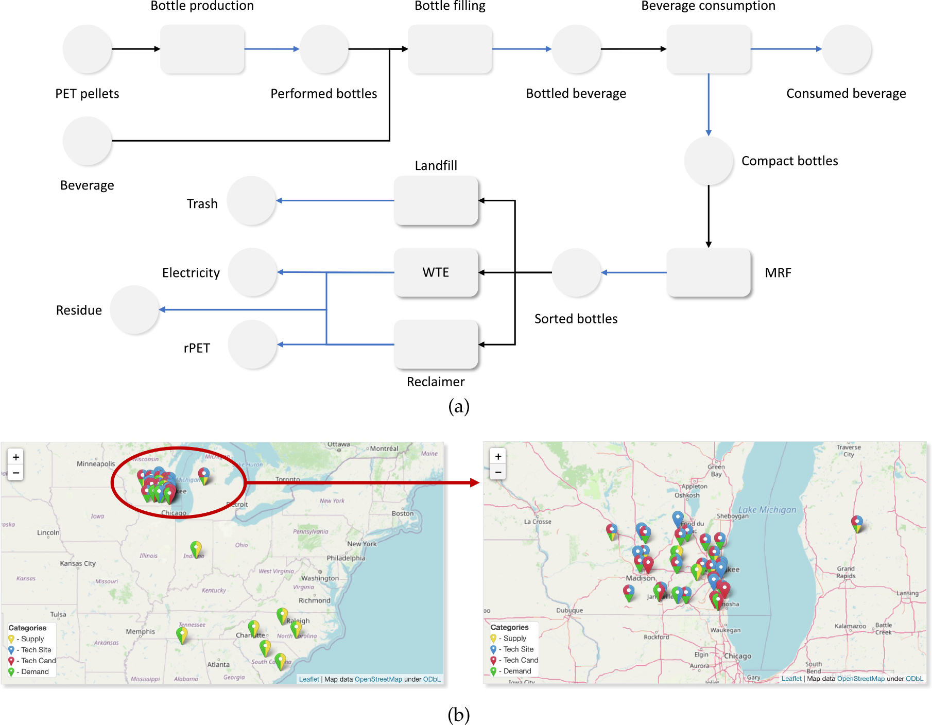
p-graph (a) and g-graph (b) for plastic recycling example.
The g-graph is shown in Fig. 15(b) exhibits the case study area, where we consider the beverage consumption in Wisconsin. Virgin PET pellets are generated outside of the state, while the material transformation is performed within the state. The detailed placement of g-graph vertices and corresponding data are obtained from the literature. There are seven virgin PET resin producers in the US, primarily located in the southwest. We considered 20 bottling facilities in Midwest providing bottled water or widely consumed beverages to consumers in the counties of Wisconsin (72 nodes). Here, we note that beverage consumption is estimated by the county populations, and consumer behavior (consumption) is represented by a technology that operates at no cost to model the corresponding material transformation. In Wisconsin, there are 25 active landfills, 30 MRFs, two waste-to-energy plants, and one PET reclamation plant considered in this study. The economic indicators such as the value of electricity (0.10708 USD/kWh) and rPET pellet (500 USD/tonne) are decided based on the current market value, which can be tuned to encourage the system to utilize plastic waste and divert it from landfills.
A couple of SC designs are shown in Fig. 16 for high and low rPET price levels, where each colored line represents transportation for different materials in the p-graph. Under market price (500 USD per metric tonne), the production of rPET is not as competitive as producing electricity or landfilling the bottles directly. When its price increase to 1000 USD per metric tonne, the reclaimer technologies are activated. For detailed documentation and results, the reader is referred to the case study available in ADAM.
Fig. 16.

Results for plastic recycling example with different rPET prices (a) 500 USD/metric tonne (b) 1000 USD/metric tonne.
6. Conclusions and future work
We have presented ADAM, a web-based tool that facilitates the modeling and solving of multi-product supply chain (SC) models. ADAM provides a highly visualized and interactive platform built on a compact graph-based modeling abstraction. The ADAM platform eliminates coding requirements, allowing users to focus entirely on model building and results analysis. The proposed graph-based model uses a p-graph and g-graph to fully represent the data and relationships defined in the mathematical formulation of the multi-product SC model. The hierarchy of SC model, p-graph and g-graph, vertices, and edges provide the possibility of achieving a scalable data and object management system. The ADAM technology database, product database, and model management system efficiently improve the flexibility, convenience, and modularity of model building. The embedded GIS visualization tool can display SC optimization results in a quick and interactive manner. A simple tutorial and a couple case studies were given to illustrate the ADAM capabilities.
In future work we plan to further enhance the visualization functions of ADAM by providing summaries of each product in the model. This could help users identify the value change along the SC for a specific material. We seek to implement a market analysis module in ADAM where users can provide their true bidding price in an organic waste market so that ADAM can clear the hypothetical market in real-time to mimic the market behavior and reveal insights for establishing a real market. Due to the complexity of multi-product SC problems, large-scale models are challenging for ADAM. Therefore, we plan to develop faster and automatic graph aggregation algorithms that can provide approximate solutions to those large models (Ma and Zavala, 2021). Moreover, we will incorporate additional modeling features such as space-time dynamics and inventory management.
Supplementary Material
Acknowledgments
We acknowledge support from the U.S. EPA (contract number EP-18-C-000016) for the development of ADAM. We acknowledge support from the U.S. Department of Agriculture (grant 2017–67003-26055) for the development of modeling abstractions and organic waste case studies implemented in ADAM. The development of the plastic waste case study was supported by the U.S. Department of Energy, Office of Energy Efficiency and Renewable Energy, Bioenergy Technologies Office under Award Number DEEE0009285. Victor Z would like to thank the undergraduate students of CBE 450: Process Design for helpful feedback on their experience using ADAM.
The views expressed in this article are those of the authors and do not necessarily reflect the views or policies of the U.S. Environmental Protection Agency. Mention of trade names, products, or services does not convey, and should not be interpreted as conveying, official U.S. EPA approval, endorsement, or recommendation.
Footnotes
Declaration of Competing Interest
This manuscript has not been submitted to, nor is under review at, another journal or other publishing venue.
The authors have no affiliation with any organization with a direct or indirect financial interest in the subject matter discussed in the manuscript
CRediT authorship contribution statement
Yicheng Hu: Methodology, Formal analysis, Software, Writing – original draft, Visualization. Weiqi Zhang: Methodology, Formal analysis, Software, Writing – original draft, Visualization. Philip Tominac: Writing – original draft, Visualization. Margaret Shen: Software, Writing – original draft, Visualization. Dilara Gorëke: Writing – original draft, Visualization. Edgar Martín-Hernández: Software, Methodology. Mariano Martín: Conceptualization, Methodology. Gerardo J. Ruiz-Mercado: Conceptualization, Methodology, Writing – original draft. Victor M. Zavala: Conceptualization, Supervision, Writing – review & editing, Funding acquisition.
Supplementary materials
Supplementary material associated with this article can be found, in the online version, at doi:10.1016/j.compchemeng.2022.107911.
References
- Abdali H, Sahebi H, Pishvaee M, 2021. The water-energy-food-land nexus at the sugarcane-to-bioenergy supply chain: a sustainable network design model. Comput. Chem. Eng. 145, 107199. [Google Scholar]
- Ballou RH, 1998. Business logistics management.
- Barbosa-Póvoa AP, 2014. Process supply chains management – where are we? where to go next? Front. Energy Res. 2, 23. 10.3389/fenrg.2014.00023. [DOI] [Google Scholar]
- Bertok B, Barany M, Friedler F, 2013. Generating and analyzing mathematical programming models of conceptual process design by p-graph software. Ind. Eng. Chem. Res. 52 (1), 166–171. [Google Scholar]
- Carpenter A, Mann M, Gelman R, Lewis J, Benson D, Cresko J, Ma S, 2014. Materials flows through industry tool to track supply chain energy demand. Proceedings of the LCA XIV International Conference, 6–8 October 2014. San Francisco, California, p. 142. [Google Scholar]
- Daher BT, Mohtar RH, 2015. Water–energy–food (WEF) nexus tool 2.0: guiding integrative resource planning and decision-making. Water Int. 40 (5–6), 748–771. [Google Scholar]
- Dueñas P, Leung T, Gil M, Reneses J, 2015. Gas–electricity coordination in competitive markets under renewable energy uncertainty. IEEE Trans. Power Syst. 30 (1), 123–131. 10.1109/TPWRS.2014.2319588. [DOI] [Google Scholar]
- Finley JW, Seiber JN, 2014. The nexus of food, energy, and water. J. Agric. Food Chem. 62 (27), 6255–6262. [DOI] [PubMed] [Google Scholar]
- Friedler F, Tarjan K, Huang Y, Fan L, 1992. Graph-theoretic approach to process synthesis: axioms and theorems. Chem. Eng. Sci. 47 (8), 1973–1988. [Google Scholar]
- Friedler F, Tarjan K, Huang Y, Fan L, 1993. Graph-theoretic approach to process synthesis: polynomial algorithm for maximal structure generation. Comput. Chem. Eng. 17 (9), 929–942. [Google Scholar]
- Garcia DJ, You F, 2015. Supply chain design and optimization: challenges and opportunities. Comput. Chem. Eng. 81, 153–170. 10.1016/j.compchemeng.2015.03.015.Special Issue: Selected papers from the 8th International Symposium on the Foundations of Computer-Aided Process Design (FOCAPD 2014), July 13–17, 2014, Cle Elum, Washington, USA [DOI] [Google Scholar]
- Goetschalckx M, 2011. Supply Chain Engineering, Vol. 161. Springer Science & Business Media. [Google Scholar]
- Haklay M, Weber P, 2008. OpenStreetMap: user-generated street maps. IEEE Pervasive Comput. 7 (4), 12–18. [Google Scholar]
- Hu Y, Scarborough M, Aguirre-Villegas H, Larson RA, Noguera DR, Zavala VM, 2018. A supply chain framework for the analysis of the recovery of biogas and fatty acids from organic waste. ACS Sustain. Chem. Eng. 6 (5), 6211–6222. [Google Scholar]
- Kraucunas I, Clarke L, Dirks J, Hathaway J, Hejazi M, Hibbard K, Huang M, Jin C, Kintner-Meyer M, van Dam KK, et al. , 2015. Investigating the nexus of climate, energy, water, and land at decision-relevant scales: the platform for regional integrated modeling and analysis (prima). Clim. Change 129 (3), 573–588. [Google Scholar]
- Lima C, Relvas S, Barbosa-Póvoa APF, 2016. Downstream oil supply chain management: a critical review and future directions. Comput. Chem. Eng. 92, 78–92. 10.1016/j.compchemeng.2016.05.002. [DOI] [Google Scholar]
- Lin T, Wang S, Rodríguez LF, Hu H, Liu Y, 2015. CyberGIS-enabled decision support platform for biomass supply chain optimization. Environ. Model. Softw. 70, 138–148. [Google Scholar]
- Ma J, Tominac P, Pfleger BF, Zavala VM, 2021. Infrastructures for phosphorus recovery from livestock waste using cyanobacteria: transportation, techno-economic, and policy implications. ACS Sustain. Chem. Eng. 9 (34), 11416–11426. [Google Scholar]
- Ma J, Zavala VM, 2021. Solution of large-scale supply chain models using graph sampling & coarsening. arXiv preprint arXiv:2111.01249. [Google Scholar]
- Martín-Hernández E, Ruiz-Mercado GJ, Martín M, 2021. A geospatial environmental and techno-economic framework for sustainable phosphorus management at livestock facilities. Resour. Recovery Recycl.Under Review [DOI] [PMC free article] [PubMed] [Google Scholar]
- Martinez-Hernandez E, Leach M, Yang A, 2017. Understanding water-energy-food and ecosystem interactions using the nexus simulation tool NexSym. Appl. Energy 206, 1009–1021. [Google Scholar]
- Mitridati L, Kazempour J, Pinson P, 2020. Heat and electricity market coordination: a scalable complementarity approach. Eur. J. Oper. Res. 283 (3), 1107–1123. 10.1016/j.ejor.2019.11.072. [DOI] [Google Scholar]
- Ng RT, Patchin S, Wu W, Sheth N, Maravelias CT, 2018. An optimization-based web application for synthesis and analysis of biomass-to-fuel strategies. Biofuels, Bioprod. Biorefin. 12 (2), 170–176. [Google Scholar]
- Pan S-Y, Du MA, Huang I-T, Liu I-H, Chang E, Chiang P-C, 2015. Strategies on implementation of waste-to-energy (WTE) supply chain for circular economy system: a review. J. Clean. Prod. 108, 409–421. [Google Scholar]
- Papageorgiou LG, 2009. Supply chain optimisation for the process industries: advances and opportunities. Comput. Chem. Eng. 33 (12), 1931–1938. 10.1016/j.compchemeng.2009.06.014.FOCAPO 2008 – Selected Papers from the Fifth International Conference on Foundations of Computer-Aided Process Operations [DOI] [Google Scholar]
- Payet-Burin R, Kromann M, Pereira-Cardenal S, Strzepek KM, Bauer-Gottwein P, 2019. WHAT-IF: an open-source decision support tool for water infrastructure investment planning within the water–energy–food–climate nexus. Hydrol. Earth Syst. Sci. 23 (10), 4129–4152. [Google Scholar]
- Reich-Weiser C, Fletcher T, Dornfeld DA, Horne S, 2008. Development of the supply chain optimization and planning for the environment (SCOPE) tool-applied to solar energy. 2008 IEEE International Symposium on Electronics and the Environment. IEEE, pp. 1–6. [Google Scholar]
- Sampat AM, Hicks A, Ruiz-Mercado GJ, Zavala VM, 2021. Valuing economic impact reductions of nutrient pollution from livestock waste. Resour. Conserv. Recycl. 164, 105199. [DOI] [PMC free article] [PubMed] [Google Scholar]
- Sampat AM, Hu Y, Sharara M, Aguirre-Villegas H, Ruiz-Mercado G, Larson RA, Zavala VM, 2019. Coordinated management of organic waste and derived products. Comput. Chem. Eng. 128, 352–363. [DOI] [PMC free article] [PubMed] [Google Scholar]
- Sampat AM, Martin E, Martin M, Zavala VM, 2017. Optimization formulations for multi-product supply chain networks. Comput. Chem. Eng. 104, 296–310. [Google Scholar]
- Sampat AM, Martin-Hernandez E, Martín M, Zavala VM, 2018. Technologies and logistics for phosphorus recovery from livestock waste. Clean Technol. Environ. Policy 20 (7), 1563–1579. [Google Scholar]
- Sampat AM, Ruiz-Mercado GJ, Zavala VM, 2018. Economic and environmental analysis for advancing sustainable management of livestock waste: a wisconsin case study. ACS Sustain. Chem. Eng. 6 (5), 6018–6031. [DOI] [PMC free article] [PubMed] [Google Scholar]
- Tominac P, Aguirre-Villegas H, Sanford J, Larson R, Zavala V, 2020. Evaluating landfill diversion strategies for municipal organic waste management using environmental and economic factors. ACS Sustain. Chem. Eng. 9 (1), 489–498. [Google Scholar]
- Tominac PA, Zavala VM, 2020. Economic properties of multi-product supply chains. Comput. Chem. Eng. 107157. 10.1016/j.compchemeng.2020.107157. [DOI] [Google Scholar]
- Varbanov PS, Friedler F, Klemes J, 2017. Process network design and optimisation using p-graph: the success, the challenges and potential roadmap. Chem. Eng. Trans. 61, 1549–1554. [Google Scholar]
- Voll P, Klaffke C, Hennen M, Bardow A, 2013. Automated superstructure-based synthesis and optimization of distributed energy supply systems. Energy 50, 374–388. [Google Scholar]
- Wu W, Henao CA, Maravelias CT, 2016. A superstructure representation, generation, and modeling framework for chemical process synthesis. AlChE J. 62 (9), 3199–3214. [Google Scholar]
- You F, Wang B, 2011. Life cycle optimization of biomass-to-liquid supply chains with distributed–centralized processing networks. Ind. Eng. Chem. Res. 50 (17), 10102–10127. [Google Scholar]
Associated Data
This section collects any data citations, data availability statements, or supplementary materials included in this article.