Estimation of multiple ordered ROC curves using placement values

Abstract

In many diagnostic accuracy studies, a priori orders may be available on multiple receiver operating characteristic curves. For example, being closer to delivery, fetal ultrasound measures in the third trimester should be no less accurate than those in the second trimester in predicting small-for-gestational-age births. Such an a priori order should be incorporated in estimating receiver operating characteristic curves and associated summary accuracy statistics, as it can potentially improve statistical efficiency of these estimates. Early work in the literature has mainly taken an indirect approach to this task and has induced the desired a priori order through modeling test score distributions. We instead propose a new strategy that incorporates the order directly through the modeling of receiver operating characteristic curves. We achieve this by exploiting the link between placement value (the relative position of a diseased test score in the healthy score distribution), the cumulative distribution function of placement value, and receiver operating characteristic curve, and by building stochastically ordered random variables through mixture distributions. We take a Bayesian semiparametric approach in using Dirichlet process mixture models so that the placement values can be flexibly modeled. We conduct extensive simulation studies to examine the performance of the proposed methodology and apply the new framework to data from obstetrics and women’s health studies.

1. Introduction

The receiver operating characteristic (ROC) curve is a graphical tool to illustrate diagnostic ability of a continuous test in predicting a binary disease status, for example diseased and healthy.¹ A useful index of diagnostic accuracy is the area under the ROC curve (AUC) that can be interpreted as the probability that a randomly selected diseased subject has a higher test score than a randomly selected healthy one.² A large body of literature exists on ROC curves in diverse fields including engineering,³ finance,⁴ economics,⁵ biomedical science,^6,7 environmental science⁸ and machine learning.⁹ Pepe¹⁰ and Zhou et al.¹¹ provide comprehensive reviews of ROC analysis and its applications.

In diagnostic studies, a priori information are often available. In obstetrics, estimated fetal weight (EFW), a measure of fetal size derived from ultrasound examinations during pregnancy, is usually used to predict certain birth weight outcomes such as small-for-gestational age (SGA).^12,13 Prior literature has shown that an EFW from an examination late in pregnancy (e.g. in third trimester) should have higher discriminatory capacity than one earlier (e.g. in second trimester).¹⁴ Such an a priori belief can be formulated as a constraint that the ROC curve of the late EFW should dominate that of the early one. As another example, in the NICHD Physician Reliability Study,¹⁵ clinical information was successively made available to physicians to diagnose endometriosis, a women’s disorder in which endometrium tissue grows outside of the uterus, using the revised American Society for Reproductive Medicine (rASRM) score.¹⁶ It is reasonable to believe that a setting with more clinical information should render higher diagnostic accuracy than one with less.¹⁷ It is well established that, when such a priori information are available, it is beneficial to incorporate them in the modeling process as they usually lead to improved statistical efficiency in estimates.¹⁸ The consideration of a priori constraints in ROC curve modeling is not new. Hanson et al.¹⁹ developed a nonparametric Bayesian approach to ROC analysis to impose the stochastic order constraint between healthy and diseased test score distributions. Kottas²⁰ considered stochastic precedence, a constraint that is less restrictive than the stochastic order. Both Hanson et al.¹⁹ and Kottas²⁰ were concerned with a single test (hence a single ROC curve) and used the constraints on the relationship between healthy and diseased test score distributions. To consider constraints in multiple tests (hence more than one ROC curves), Hwang and Chen¹⁷ proposed an integrated method to impose both stochastic and variability orders^21,22 with the former applied to the relationship between healthy and diseased test score distributions within each test and the latter to the relationship between the multiple test score distributions within either the healthy or diseased population. While useful, these existing approaches formulated a priori constraints between test score distributions, and hence are not desirable when constraints are between ROC curves. In the aforementioned obstetrics study, the a priori belief concerns the relationship between ROC curves of an early and a late ultrasound EFW, not the relationship between EFW distributions of SGA and non-SGA cohort within the early or late ultrasound examination. Similarly, the a priori constraint in the Physician Reliability Study is formulated as the relationship between two settings with different clinical information, not as the relationship between rASRM score distributions of women with and without endometriosis within each setting. Clearly, it is desirable to have a framework where a priori constraints can be considered directly on the ROC curves.

In this paper, we exploit the idea of placement value (PV).²³ Briefly, PV is a standardization of the diseased test score with respect to the healthy test score distribution. A nice and important feature of the PV-based ROC analysis is that the ROC curve of a test is simply the cumulative distribution function (CDF) of the PV random variable associated with the test. As such, two tests with ordered ROC curves can be viewed as two tests with their PV random variables stochastically ordered. With this novel connection, the complicated and indirect process of imposing constraints on ROC curves through test score distributions, as implemented in Hwang and Chen,¹⁷ can be replaced by working with stochastically ordered random variables, a task that is direct and straightforward. PV-based ROC analytical approaches have been considered by various authors.^24–28 None of them, however, considered ordered ROC curves.

The adoption of the PV framework for modeling ordered ROC curves also makes it possible to include covariates and assess their effects on ROC curves. In this article, we take a Bayesian semiparametric approach to ROC analysis using Dirichlet process mixture (DPM) models²⁹ to provide flexibility in the estimations. DPM has been proven useful to estimate distribution functions^30–32 and has been extended to adjust for covariates.^33–36 The rest of the article is organized as follows. Section 2 provides the detailed development of the proposed method on stochastically ordered ROC curves with and without covariates using placement values. We demonstrate the performance of the developed methodology through simulations in Section 3. In Section 4, we illustrate the utility of the proposed framework using both an EFW dataset in obstetrics and a dataset from the Physician Reliability Study. We conclude with a brief discussion in Section 5.

2. Methods

2.1. ROC curves and placement values

Let Y⁰ and Y¹ represent continuous test scores from a healthy and a diseased population, respectively, with corresponding CDFs F₀ and F₁. The ROC curve is a graphical relationship between the true positivity rate, or sensitivity, and the false positivity rate, or one minus specificity, at all possible cut-off points. Given data ${\mathit{y}}^0=\left(y_1^0,,y_m^0\right)$ and ${\mathit{y}}^1=\left(y_1^1,,y_n^1\right)$ from F₀ and F₁, respectively, where m and n are the corresponding sample sizes, one can estimate F₀ and F₁ and subsequently estimate ROC using $ROC\left(t\right)=1-F_1\left(F_0^{-1}\left(1-t\right)\right),t\in \left(0,1\right)$, where F⁻¹(t) is the inverse function of F(t).

Alternatively, DeLong et al.²³ suggests estimating F₀ and obtaining placement values $z_i=P\left(Y^0>y_i^1\right)=1-F_0\left(y_i^1\right)$, i = 1, , n; see also Pepe³⁷ and Pepe and Cai.²⁶ Let Z be the random variable for the PV. It is easy to show that the ROC curve is simply the CDF of Z.²⁶ This alternative way of estimating ROC curves provides a new perspective in considering a priori constraints, as we develop below.

2.2. Semiparametric modeling of the placement values

Assume for now placement values z = (z₁, , z_n) are available; Section 2.4 will describe how to use Bayesian semiparametric methods to estimate PVs. We model the CDF F of z semiparametrically using DPM by specifying, for i = 1, , n,

$$\begin{array}{l}F\left(z_i\mid {\mu }_i,{\sigma }^2\right)=\int \mathbb{K}\left(z_i;{\mu }_i,{\sigma }^2\right)dH\left({\mu }_i\right),\\ H\left({\mu }_i\right)\sim 𝒟\left(\alpha H_0\left({\mu }_i\right)\right),\end{array}$$ (1)

where H is a mixing probability measure, $𝒟\left(\alpha H_0\right)$ denotes a Dirichlet process (DP)³⁸) with base measure H₀ and precision α, and kernel $\mathbb{K}\left(\cdot ;\mu ,{\sigma }^2\right)$ is a distribution function with parameters μ and σ².

Following the constructive representation of a DP as a stick-breaking process³⁹ and using a Gaussian kernel and a Gaussian base measure, we can model z as

$$\begin{array}{l}\eta \left(z_i\right)~N\left({\mu }_i,{\sigma }^2\right),\\ {\mu }_i~H,H=\sum _k{p}_k{\delta }_{{\mu }_k^{*}},\\ p_k=V_k\prod _{l<k}\left(1-V_l\right),V_k~Beta(1,\alpha ),\\ {\mu }_k^{*}~N\left({\mu }_0,{\sigma }_0^2\right),\end{array}$$ (2)

where η is a pre-specified monotone increasing transformation (e.g. logit) that maps the placement value on (0, 1) onto the real line $\Re$, $N\left(\mu ,{\sigma }^2\right)$ denotes a normal distribution with mean μ and variance σ², Beta(α₁, α₂) denotes a beta distribution with shape parameters α₁ and α₂, δ_c is a point mass at c, μ₀, and ${\sigma }_0^2$ are unknown hyperparameters, V_k ’s are the “stick” lengths, p_k ’s are the mixing weights, and k indexes clusters. When restricting the model dimension to finite so that k = 1, . . ., K < ∞, we obtain the truncated stick-breaking process. It has been shown that the truncated stick-breaking process provides accurate approximation when K is moderate, say K = 30.⁴⁰ A well-established strength of the above Dirichlet process mixture is its ability to model flexible distributions. This feature suits the modeling of placement values particularly well. It is our experience that ROC curve and AUC estimates are sensitive to tail behaviors of the PV distributions and that PVs after η transformation still exhibit skewness and heavy tails.^41,42 In (2), we have chosen to mix with the location parameter only. As pointed out in the literature,^43,44 any density on the real line can be approximated using a Dirichlet process location mixture of normals.

The model in (2) can be fit straightforwardly with a Markov chain Monte Carlo (MCMC) algorithm.⁴⁵ With a sample ${\widehat{p}}_1^{(l)},\dots ,{\widehat{p}}_K^{\left(l\right)}$, ${\widehat{\mu }}_1^{*\left(l\right)}$, , ${\widehat{\mu }}_K^{*\left(l\right)}$, and ${\widehat{\sigma }}^{\left(l\right)}$ at the l^th MCMC iteration, the ROC curve can be estimated as

$${\widehat{ROC}}^{\left(l\right)}\left(t\right)=\sum _{k=1}^K{\widehat{p}}_k^{\left(l\right)}\text{Φ}\left(\frac{\eta \left(t\right)-{\widehat{\mu }}_k^{*\left(l\right)}}{{\widehat{\sigma }}^{\left(l\right)}}\right),t\in \left(0,1\right),$$

where Φ(·) is the CDF of the standard normal distribution. With L iterations, the posterior mean of the ROC curve can be obtained as the corresponding averages. AUC estimates can be consequently estimated by the Trapezoidal rule. Variability measures (posterior standard deviations or credible intervals) of these estimates can be obtained easily through the MCMC sample as well.

2.3. Stochastically ordered ROC curves

We now consider J tests, whose ROC curves are believed to be ordered a priori as

$$RO{C}_1\left(t\right)\le \cdots \le RO{C}_J\left(t\right),\text{ for all }t\in \left(0,1\right).$$ (3)

Suppose for the j^th test, healthy scores ${\mathit{y}}_j^0=\left(y_{j1}^0,\dots ,y_{j{m}_j}^0\right)$ and diseased scores ${\mathit{y}}_j^1=\left(y_{j1}^1,\dots ,y_{j{n}_j}^1\right)$ are available, where m_j and n_j are the corresponding sample sizes, respectively. Let the PVs of the J tests be Z₁, . . ., Z_J, where ${\mathit{\text{Z}}}_j=\left(Z_{j1},\dots ,Z_{j{n}_j}\right)$, j = 1, . . ., J. The a priori constraint in (3) implies P(Z_1k ≤ z) ≤ . . . ≤ P(Z_Jk ≤ z) for all z ∈ (0, 1), k. For this reason, we call (3) stochastically ordered ROC curves.

Similar to Section 2.2, assume for now PVs ${\mathit{\text{z}}}_j=\left(z_{j1},\dots ,z_{j{n}_j}\right)$, j = 1, . . ., J are available. In the absence of any a priori order, the J ROC curves can be estimated through the model formulation

$$\begin{array}{l}\eta \left(z_{ji}\right)~N\left({\mu }_{ji},{\sigma }_j^2\right),\\ {\mu }_{ji}~H_j,H_j=\sum _k{p}_k{\delta }_{{\mu }_{jk}^{*}},\\ p_k=V_k\prod _{l<k}\left(1-V_l\right),V_k~Beta\left(1,\alpha \right),\end{array}$$ (4)

with the base measure specified as

$${\mu }_{jk}^{*}~N\left({\mu }_{j0},{\sigma }_{j0}^2\right),$$ (5)

for j = 1, ..., J . Here, all notations are defined similarly as in (2), and all have the j subscript to index test, except the mixing weights p₁, . . ., p_K. The shared mixing weights across the J tests induce dependence among the J ROC curves ROC₁, . . ., ROC_J, hence effectively account for the possible correlation in the observed test scores.

To incorporate the stochastic order constraint (3), we require ${\mu }_{1k}^{\ast }\ge \dots \ge {\mu }_{Jk}^{\ast }$ at all k and ${\sigma }_1^2=\dots ={\sigma }_J^2={\sigma }^2$. The former can be achieved by replacing (5) with

$$\begin{array}{l}{\mu }_{jk}^{*}=\sum _{l=1}^J{\beta }_{lk}I\left(l\le j\right),\\ {\beta }_{1k}~N\left(a_1,b_1^2\right),\\ {\beta }_{jk}~N_{-}\left(a_j,b_j^2\right),j=2,\dots ,J.\end{array}$$ (6)

Here I(c) is an indicator function that takes value 1 if condition c is true and 0 otherwise, N_(a, b²) is the normal distribution with mean a and variance b² truncated to be negative, and a_j’s and b_j’s are unknown hyperparameters. The specifications in (6) ensure the ordering of the ${\mu }_{jk}^{\ast }$’s. For example, in the case of J = 2, ${\mu }_{1k}^{\ast }={\beta }_{1k}$ and ${\mu }_{2k}^{\ast }={\beta }_{1k}+{\beta }_{2k}$. In this case, a negative β_2k ensures ${\mu }_{1k}^{\ast }\ge {\mu }_{2k}^{\ast }$, which in turn ensures P(Z₁ < t) ≤ P(Z₂ < t), hence ROC₁(t) ≤ ROC₂(t).

The following summarizes the result. See also Kottas and Gelfand,⁴⁶ Dunson and Peddada,⁴⁷ and Hoff.⁴⁸

Result 2.1. Suppose η(·) is a known monotone increasing function from (0, 1) onto $\Re$. Then model formulations (4) and (6) are sufficient for (3).

Proof. A brief proof is provided in Section 1 of Supplemental Material, available online. □

2.4. Integrating the process of estimating PVs

We have so far assumed that placement values z_j’s are available and known. In reality, however, they have to be estimated by using test scores of both healthy (for estimating the F₀’s) and diseased (for computing PVs) populations. To be consistent with using DPM to model the placement values, we also use DPM to model the healthy test scores ${\mathit{\text{y}}}_j^0$ in order to estimate the placement values z_j. Specifically, for i = 1, . . ., m_j, j = 1, . . ., J, we assume the following truncated stick breaking process

$$\begin{array}{l}{y}_{ji}^0~N\left({\theta }_{ji},{\tau }_j^2\right),{\theta }_{ji}~Q_j,Q_j=\sum _{k=1}^K{\pi }_k{\delta }_{{\theta }_{jk}^{*}},\\ {\pi }_k={\nu }_k\prod _{l<k}\left(1-{\nu }_l\right),{\nu }_k~Beta\left(1,{\alpha }_0\right),\\ {\theta }_{jk}^{*}~N\left({\theta }_{j0},{\lambda }_j^2\right),k=1,\dots ,K,\end{array}$$ (7)

where Q_j’s are mixing probability measures, π_k ’s are mixing weights, ${\nu }_k$’s are stick lengths and θ _j0 and ${\lambda }_j^2$ are mean and variance of the normal base measures.

Again, the shared mixing weights π_k ’s effectively account for the possible correlations between $y_{ji}^0$ and $y_{j^{\prime }i}^0$ for $j\ne j^{\prime }$. Using an MCMC algorithm similar to that in Section 2.2, we can obtain a sample from the posterior distribution of the model parameters. Given the l^th sample from L₀ iterations ${\widehat{\theta }}_{j1}^{*\left(l\right)},\dots ,{\widehat{\theta }}_{jK}^{*\left(l\right)}$, ${\widehat{\pi }}_1^{*\left(l\right)},\dots ,{\widehat{\pi }}_K^{*\left(l\right)}$, and ${\widehat{\tau }}_j^{\left(l\right)}$, the PVs can be estimated as

$${\widehat{z}}_{ji}^{\left(l\right)}=1-{\widehat{F}}_{j0}^{\left(l\right)}\left(y_{ji}^1\right)=1-\sum _{k=1}^K{\widehat{\pi }}_k^{\left(l\right)}\text{Φ}\left(\frac{y_{ji}^1-{\widehat{\theta }}_{jk}^{*\left(l\right)}}{{\widehat{\tau }}_j^{\left(l\right)}}\right),$$

where ${\widehat{F}}_{j0}\left(y\right)$ is the estimate of $F_{j0}\left(y\right)$, the CDF of $y_{ji}^0$.

2.5. Covariate-specific ROC analysis

In practice, covariates can impact the prediction ability of the test. Let W⁰ and W¹ be vectors of covariates for diseased and healthy populations, respectively. The covariate-specific ROC curve given a covariate value w is defined as

$$ROC\left(t\mid \mathit{\text{w}}\right)=1-F\left(F_0^{-1}\left(1-t\mid {\mathit{\text{W}}}^0=\mathit{\text{w}}\right)\mid {\mathit{\text{W}}}^1=\mathit{\text{w}}\right),$$ (8)

where F(t|W = w) is a CDF conditional on w. The covariate-specific AUC is similarly defined as

$$AUC(\mathit{\text{w}})={\int }_0^{1}ROC\left(t\mid \mathit{\text{w}}\right)dt.$$

Let z_w be the covariate-specific placement value so that

$$z_{\mathit{\text{w}}}=P\left[Y^0>y^1\mid \mathit{\text{w}}\right]=1-F_0\left(y^1\mid \mathit{\text{w}}\right).$$

Then (8) can be re-written as

$$ROC(t\mid \mathit{\text{w}})=P\left[z_{\mathit{\text{w}}}<t\mid \mathit{\text{w}}\right].$$ (9)

Accordingly, estimation of covariate-specific ROC curves can be implemented by incorporating w in both the PV estimation stage (Stage 1) and the ROC estimation stage (Stage 2). The former will produce z_w and the latter ROC(t|w). Using DPM, Stage 1 is a simple extension of (7), with the base measure replaced by ${\theta }_{jk}^{*}~N\left({\theta }_{j0}+{\mathit{\gamma }}_0^T{\mathit{\text{W}}}^0,{\lambda }_j^2\right)$. Similarly, Stage 2 extends (4) and (6) with the new base measure ${\mu }_{jk}^{*}={\sum }_{l=1}^J{\beta }_{lk}I\left(l\le j\right)+{\mathit{\text{γ}}}_1^T{\mathit{\text{W}}}^1$. As such, the stochastic order constraint (3) applies to ROC curves at a given covariate value w:

$$RO{C}_1\left(t\mid \mathit{\text{w}}\right)\le \cdots \le RO{C}_J\left(t\mid \mathit{\text{w}}\right)\text{, for all }t\in \left(0,1\right).$$

2.6. Bayesian computational considerations

We use proper but vague priors for all model parameters. In particular, we use univariate normal distribution N(0, 1000) for regression coefficients θ _j0, a_j, j = 1, . . ., J, multivariate normal distribution N(0, 1000I ) for γ₀ and γ₁, where 0 and I are vector of zeros and identity matrix, respectively, of length or dimension conforming to W⁰ and W¹, Gamma distribution G(0.01, 0.01) for the reciprocals of τ_j, ${\sigma }_j^2$, ${\lambda }_j^2$ and $b_j^{2}j=1,\dots ,J$, and G(1, 1) for α₀ and α. Here G(α, β) denotes the gamma distribution with shape α and rate β. We assumed that these parameters are all independent a priori.

We develop an MCMC algorithm to generate samples from the posterior distribution of the model parameters given the data. Both visual inspection of the trace plots and diagnostic tools⁴⁹ are used to ensure convergence of the MCMC chain. After convergence, we thin the iterations to obtain a sample of 5000 iterations to produce posterior means, standard deviations and 95% credible intervals. The algorithm is implemented in R.⁵⁰

3. Simulations

In this section, we present simulation studies to illustrate the performance of the proposed modeling framework. These simulations are carried out without covariate in Section 3.1 and with covariates in Section 3.2.

3.1. Simulation with no covariate

We consider two tests (Test 1 and Test 2) with healthy ($Y_1^0$ and $Y_2^0$) and diseased ($Y_1^1$ and $Y_2^1$) scores from the following data generating mechanism

$$\begin{array}{l}{Y}_j^0~N\left({\mu }_j^0,{\left({\sigma }_j^0\right)}^2\right)\\ Y_j^1~N\left({\mu }_j^1,{\left({\sigma }_j^1\right)}^2\right),\end{array}$$ (10)

where j = 1, 2 indexes the tests, ${\mu }_j^0$, ${\mu }_j^1$ and ${\sigma }_j^0$, ${\sigma }_j^1$ are pre-specified means and variances of healthy and diseased test scores distributions, respectively. Under this setup, PVs are computed as

$$z_j=1-\text{Φ}\left(\frac{y_j^1-{\mu }_j^0}{{\sigma }_j^0}\right),$$

where $y_j^1$ is a realization of $Y_j^1$.

By varying the true values of ${\mu }_j^0$, ${\sigma }_j^0$, ${\mu }_j^1$, and ${\sigma }_j^1$ in (10), we create cases where the two ROC curves are either stochastically ordered (ROC₁ ≤ ROC₂) or unordered. For each case, we allow different levels of separation between ROC curves (low, medium, high), and generate n₁ = n₂ = n PVs with n = 150, 250, 500. Table 1 of Supplemental Material displays these six scenarios and the associated values of μ’s and σ’s. We fit our proposed model (SO) and its unconstrained counterpart (NO) to the generated PV data. We create 1000 data replicates and report average posterior means, biases, and average posterior standard deviations of AUC estimates. We also report the posterior means, biases, and average posterior standard deviations of difference of AUCs from test 2 and test 1. We also plot posterior mean estimates of ROC curves from 200 randomly selected data replicates. The simulation results with n = 150 are tabulated in Table 1, with the corresponding ROC curve estimates shown in Figure 1 of Supplemental Material, available online.

Table 1.

Summary of AUC estimates across 1000 datasets in simulations with no covariate (n = 150). Mean: posterior mean of AUC, SD: average posterior standard deviations, NO: no constraint, SO: stochastic ordering constraint that Test 1 has lower accuracy than Test 2.

ROC relation	ROC separation	Model	Test 1				Test 2				Difference
			True AUC	Mean	Bias	aSD	True AUC	Mean	Bias	aSD	True	Mean	Bias	aSD
Ordered	Low	NO	0.638	0.638	0.000	0.022	0.664	0.661	−0.003	0.022	0.026	0.024	−0.003	0.029
		SO		0.630	−0.008	0.020		0.670	0.006	0.019		0.040	0.014	0.017
	Medium	NO	0.638	0.638	−0.001	0.022	0.802	0.794	−0.008	0.019	0.164	0.157	−0.007	0.027
		SO		0.637	−0.001	0.023		0.796	−0.006	0.018		0.158	−0.006	0.027
	High	NO	0.638	0.638	−0.001	0.022	0.983	0.963	−0.020	0.008	0.345	0.325	−0.020	0.022
		SO		0.632	−0.006	0.023		0.973	−0.010	0.005		0.341	−0.004	0.021
Unordered	Low	NO	0.638	0.638	−0.001	0.022	0.650	0.646	−0.004	0.024	0.011	0.008	−0.003	0.031
		SO		0.619	−0.019	0.020		0.662	0.013	0.020		0.044	0.032	0.016
	Medium	NO	0.673	0.671	−0.002	0.020	0.704	0.693	−0.011	0.028	0.031	0.022	−0.009	0.032
		SO		0.605	−0.068	0.023		0.717	0.013	0.022		0.112	0.081	0.021
	High	NO	0.961	0.942	−0.019	0.011	0.952	0.924	−0.028	0.015	−0.009	−0.018	−0.009	0.014
		SO		0.918	−0.043	0.012		0.945	−0.007	0.008		0.027	0.036	0.006

When the true ROC curves are ordered, NO and SO models produce AUC estimates that are similar in magnitude and of the same direction (Test 1 less accurate than Test 2; Table 1). However, SO results in lower SDs, suggesting improved statistical efficiency when ordering constraint is incorporated. For example, when ROC separation is “Low,” Test 1 has lower AUC estimates than Test 2 in both NO (0.638 vs. 0.661) and SO (0.630 vs. 0.670) models, but, SO produces smaller SDs in both tests, resulting in efficiency gains of around 9% and 14% in Tests 1 and 2, respectively. The efficiency gain in estimation of the differences of test 2 and test 1 AUCs are also visible in the last column of the Table 1. On the other hand, when the true ROC curves are unordered, the proposed SO model enforces the a priori constraint so that the estimates conform to the prior belief. For example, when the ROC separation is “High,” NO model produces higher AUC estimates in Test 1 than 2 (0.942 vs. 0.924) while SO reverses the direction (0.918 vs. 0.945). The last row of Figure 1 of Supplemental Material illustrates this reversal phenomenon clearly.

Simulation results with sample sizes n = 250 and 500 are provided in the Supplemental Material, in Tables 2 and 3 (AUCs) and Figures 2 and 3 (ROCs). Similar conclusions from the primary case (n = 150) hold. We note that as sample size increases, the statistical efficiency gains under SO become more pronounced.

Figure 2.

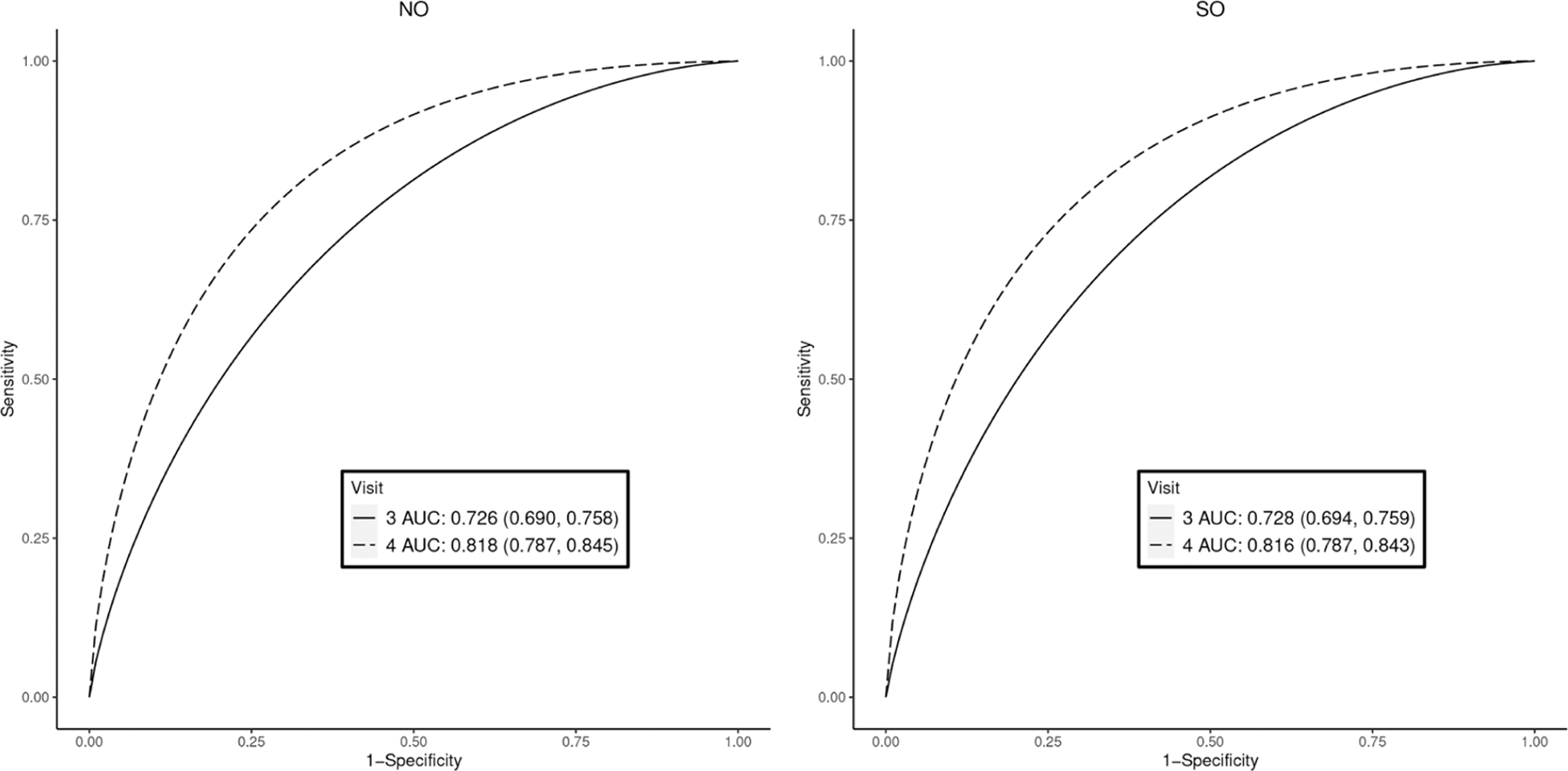
AUC estimates and ROC curves to discriminate small-for-gestational-age using estimated fetal weight, the Fetal Growth Studies. NO: no constraint; SO: stochastically ordered constraint that visit 4 has higher accuracy than visit 3. Posterior mean (95% credible intervals) are reported in the legend boxes for each visit.

Figure 3.

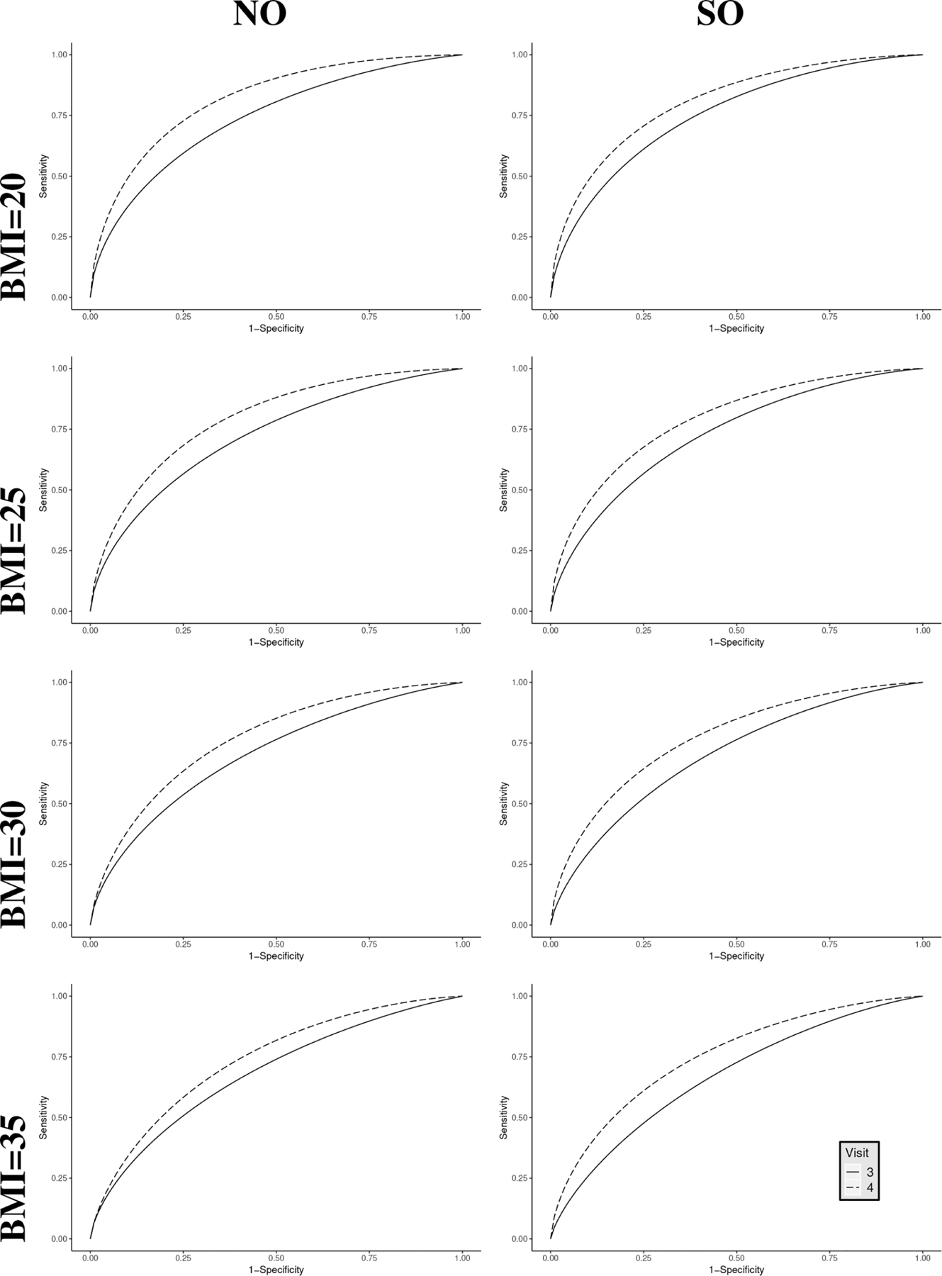
Estimated ROC curves to discriminate small-for-gestational-age at visits 3 and 4 at different values of BMI, the Fetal Growth Studies. NO: no constraint; SO: stochastically ordered constraint that visit 4 has higher accuracy than visit 3.

3.2. Simulation with covariate

In this setting, we generate a covariate W from the uniform distribution on unit interval and generate diseased scores from

$$y_j^1~N\left(\frac{1}{{\alpha }_{j1}}\left({\alpha }_{j0}+{\beta }_{j}W\right),\frac{1}{{\alpha }_{j1}^2}\right),$$

where j = 1, 2 indexes tests 1 and 2, respectively. Assuming that the healthy scores follow standard normal distribution, we generate the PVs as

$$z_j=1-\text{Φ}\left(y_j^1\right),j=1,2.$$

Similar to Section 3.1, we consider two ROC relations (stochastically ordered and unordered). Table 4 of Supplemental Material provides the values of α_j0, α_j1, and β _j used in this simulation study. In each relation, we consider covariate values (0.2, 0.5, and 0.8) to provide various levels of separation between the ROC curves. Similar to Section 3.1, we simulate n PVs with n = 150, 250, 500. We generate 1000 data based on the above setup and for each of the 1000 data, we fit both NO and SO models. Table 2 of this paper and Figure 4 of Supplemental Material contain results for sample size n = 150.

Overall, the results in Table 2 and Figure 4 of Supplemental Material track those in Table 1 of this paper and Figure 1 of Supplemental Material. In particular, when the true ROCs are unordered, NO and SO produce similar estimates with elevated efficiency gain in the SO model. For example, when the covariate value is 0.2, Test 1 has lower AUC estimates than Test 2 for both NO (0.797 vs. 0.864) and SO (0.802 vs. 0.860) models. However, SO model produces AUCs with lower SDs as compared to its NO counterpart, resulting in efficiency gains of around 17% and 16% in Test 1 and Test 2, respectively. When the true ROCs are unordered, SO model produces estimates of AUCs and ROCs that satisfy the a priori constraint. For example, when covariate value is 0.8, although NO model produces higher AUC for Test 2 (0.935 vs. 0.945), the corresponding ROC estimates intersect. On the other hand, the SO model not only produces higher AUC estimate for Test 2 (0.918 vs. 0.926), it ensures that the corresponding ROC estimates are strictly stochastically ordered. The last row of Figure 4 of Supplemental Material illustrates this.

Results are similar for the other two sample sizes (n = 250 and 500) and are reported in Tables 5 and 6 and Figures 5 and 6 of Supplemental Material online.

4. Real data examples

4.1. The Physician Reliability Study

Endometrios is a disorder with tissues that are normally inside the uterus growing outside. The NICHD Physician Reliability Study (PRS) examined accuracy of diagnosing endometriosis under settings of different amount of clinical information and by physician of different level of experiences. The PRS consisted of four successive settings and involved three groups of physicians. We focus on a subset of the PRS data in this analysis, in particular the first two settings and consider only scores of the regional expert physicians. Of note, setting 1 in PRS provides intrauteral digital images, while setting 2 adds surgeon notes on top of setting 1. This gives rise to the final subset of the data that contains information of 113 participants in setting 1 and 126 participants in setting 2. Detailed descriptions of the study design and some main findings can be found elsewhere.^15,17 The regional experts consist of four OB/GYN physicians. Following Hwang and Chen,¹⁷ we use the average rASRM scores of them as the test score in our analysis.

An interesting feature of the PRS design is that clinical information is sequentially augmented, and can be treated as a prior belief that diagnostic accuracy in a later setting (say, setting 2) is higher than an early one (say, setting 1). Let ROC₁ and ROC₂ be the ROC curves of Settings 1 and 2, respectively. This prior belief can be formulated as ROC₁(t) ≤ ROC₂(t) for all t ∈ (0, 1). We fit the SO model to the PRS data with this prior belief as a constraint and compare the results with those from the NO model that is free of this a priori constraint. To obtain PVs, we estimate the CDFs of healthy test scores from the two settings using equation (7). Then the PVs are calculated as

$$z_j=1-\sum _{k=1}^K{\widehat{\pi }}_k\text{Φ}\left(\frac{y_j^1-{\widehat{\theta }}_{jk}^{*}}{{\widehat{\tau }}_j}\right),j=1,2,$$ (11)

where ${\widehat{\pi }}_k$ are common mixing weights, ${\widehat{\theta }}_{jk}^{*}$ is the posterior mean from the k^th cluster and j^th setting for the healthy score distribution, and ${\widehat{\tau }}_j$ is the posterior variance from the j^th setting for healthy distribution. The NO and SO models are then fit to the estimated PVs, and the corresponding posterior estimates of AUCs and ROC curves are reported in Figure 1.

Figure 1.

AUC estimates and ROC curves to discriminate endometriosis using rASRM scores, the Physicians Reliability Study. NO: no constraint, SO: stochastically ordered constraint that setting 2 has higher accuracy than setting 1. Posterior mean (95% credible intervals) are reported in the legend boxes for each setting.

Results from Figure 1 suggest that, overall, the regional expert physicians are mostly accurate in diagnosing endometriosis in both settings 1 and 2, with the estimated AUCs from 0.793 to 0.826. While the regional experts are slightly better in setting 1 than 2 (0.826 vs. 0.802) according to the NO model, they are slightly worse in setting 1 than 2 (0.793 vs. 0.818) by the SO model. The reversal of direction in AUCs is also illustrated in the ROC curves. In the NO model, the two curves cross, with the ROC curve of setting 1 about the same as that of setting 2 at high specificity level, rising above afterwards until about 0.5 specificity, then decreasing below. In contrast, the ROC curve of setting 1 always stay below that of setting 2 in the SO model.

4.2. The Fetal Growth Studies

The NICHD Fetal Growth Studies (FGS) is an epidemiologic study that aimed to establish a standard for normal fetal growth and size for gestational age in the U.S. population and improve estimation accuracy of fetal weight.⁵¹ The cohort had five ultrasound examination visits during pregnancy at pre-defined gestational weeks. Using Hadlock’s formula,⁵² measurements (abdominal circumference, head circumference and femur length) from these ultrasound examinations were converted into the estimated fetal weight (EFW), a useful score for predicting abnormal birth weight categories, such as small-for-gestational age (SGA). SGA birth corresponds to the birth weight below the 10^th percentile at a given gestation,⁵³ and carries potential neonatal risks of respiratory distress syndrome, necrotizing enterocolitis, chronic lung disease, neurologic disease, and death from infection.^54,55 The FGS data consist of 2054 pregnancies with 191 SGA births. It has been previously demonstrated that an EFW from ultrasounds closer to delivery has better discriminatory capacity for the abnormal birth weights than one farther.¹⁴ This information can be translated into a stochastic order constraint that the diagnostic accuracy of an EFW at a later visit (say visit 4) is higher than that at an early one (say visit 3). To that end, we fit both NO and SO models to the FGS data from visits 3 and 4 and examine the diagnostic parameter estimates of EFWs in discriminating SGA births from normal ones. PVs were estimated in a similar fashion as described in equation (11) for the PRS data (Section 4.1).

The posterior estimates of AUCs and ROC curves are reported in Figure 2. Unlike in the PRS analysis, NO and SO models applied to FGS data produce similar AUC estimates at both visits. This similarity is a reflection that the FGS data agree with the a priori constraint that visit 4 provides better discriminating capacity than visit 3. The ROC curve estimates also confirm this finding. Note that the two ROC curves are already ordered in the NO model. As expected, we observe some statistical efficiency gains when the constraint is considered, as reflected in the narrower credible intervals in the SO model. For example, both NO (0.726 and 0.818) and SO (0.728 and 0.816) models estimate similar AUCs for visits 3 and 4, respectively, and the SO model achieves 7% and 3% efficiency gains in AUC estimates at visits 3 and 4, respectively.

It is of interest to assess whether the diagnostic accuracy of EFW is associated with important covariates such as maternal body mass index (BMI). Maternal obesity might impede the performance of ultrasound measures, which in turn could affect the accuracy of EFW in predicting SGA. To obtain PVs, we estimate covariate-specific CDFs of the non-SGA EFWs at the two visits following procedures in Section 2.5. In particular, the PVs are calculated as

$$z_j=1-\sum _{k=1}^K{\widehat{\pi }}_k\text{Φ}\left(\frac{y_j^1-{\widehat{\theta }}_{jk}^{*}-{\widehat{\gamma }}_{j0}BMI}{{\widehat{\tau }}_j}\right),j=1,2,$$

where ${\widehat{\gamma }}_{j0}$ is estimated coefficient for BMI in setting j. We then fit both NO and SO models to the estimated PVs and report AUC and ROC estimates at BMI levels of 20, 25, 30, and 35 kg/m² in Figure 3 and Table 3, respectively. In both steps (estimation of PV and modeling PV), we used linear function of BMI due to its better goodness-of-fit compared to models with quadratic structure in BMI and to models adjusting for heteroskedasticity.

Table 3.

Posterior mean AUC and 95% CIs for discriminating small-for-gestational-age using estimated fetal weight at different levels of BMI, the Fetal Growth Studies. NO: no constraint; SO: stochastically ordered constraint that visit 4 has higher accuracy than visit 3, Mean: posterior mean; CI: credible interval

BMI (kg/m2)	Visit	NO			SO
		Mean	95% CI	Mean	95% CI
20	3	0.707	(0.658, 0.753)	0.711	(0.672, 0.748)
	4	0.782	(0.739, 0.821)	0.779	(0.744, 0.813)
25	3	0.725	(0.690, 0.760)	0.726	(0.692, 0.756)
	4	0.799	(0.768, 0.827)	0.798	(0.769, 0.826)
30	3	0.742	(0.694, 0.786)	0.739	(0.697, 0.778)
	4	0.814	(0.774, 0.851)	0.815	(0.781, 0.849)
35	3	0.757	(0.684, 0.820)	0.753	(0.693, 0.805)
	4	0.828	(0.767, 0.879)	0.832	(0.786, 0.873)

As in the above analysis of FGS data without covariates, when BMI is considered, the consideration of the a priori constraint does not change the direction of AUCs and ROC curves between visits 3 and 4. However, it does lead to improved statistical efficiency in SO estimates at all the covariate levels, as is evident in the narrower credible intervals. For example, at BMI level of 20 kg/m², the estimated AUCs at visits 3 and 4 under SO model have 20% and 16% narrower CIs than those under NO model. A similar pattern is observed at other levels of BMI. It is interesting to note that the diagnostic capacity of EFW increases with BMI, possibly because variability in ultrasound measurements decreases with BMI.

5. Discussion

In this paper, we proposed a semiparametric approach to stochastically ordered ROC curves using placement values. Although stochastic orders have been considered in ROC analysis before, they were imposed on the distributions of the healthy and diseased test scores. Thus, the constraints were not directly reflected on the ROC curves. The use of placement values allows the assessment of the direct covariate impact on the ROC curves, which facilitates estimating diagnostic accuracy for a particular sub-population of interest. For instance, the obstetrics example in Section 4.2 assessed the capacity of EFW as a biomarker to predict SGA for populations with different levels of maternal BMI.

The objective of the proposed model was to impose stochastic order constraint on ROC curves given a priori belief. If the data do not agree with the constraint, the proposed model ensures that the estimated diagnostic parameters reflect the constraint. On the other hand, when the data agree with the belief, the proposed model estimates the diagnostic parameters with higher statistical efficiency than the un-constrained counterpart. Both our simulations and real data examples confirmed these. Additionally, the semiparametric approach provides a flexible framework to model the ROC curves, providing a robust method against unusual distributions in placement values.

The a priori constraint in this paper requires ROC₁(t) ≤ . . . ≤ ROC_J(t) for all t ∈ (0, 1). This is a strong assumption. A less stringent constraint is the partial AUC ordering: ${\int }_0^{s}RO{C}_1\left(t\right)dt\le \dots \le {\int }_0^{s}RO{C}_J\left(t\right)dt\text{ for all }s,t\in \left(0,1\right)$. This constraint requires ordering in all partial AUCs but allows the overall ROC curves to cross. We are currently developing estimation procedures to incorporate the partial AUC order constraint in ROC analysis. It is also of interest to consider the a priori order constraint on covariate-adjusted ROC curves.⁵⁶ Despite its novel advantages, the proposed model has a limitation common to any 2-stage approach. In stage 2 of the proposed model, we used the placement value as data and disregarded the uncertainty associated with them when they were estimated in stage 1. This in turn under-estimates the variability of the diagnostic accuracy measures in stage 2 and produces coverage probabilities that are below the nominal level. One possible remedy is a brutal-force procedure that a) generates a sample (say, L₀) of PVs from their posterior distributions in the first stage, b) repeats the second stage (estimating AUCs) using each of the PV samples in a) to obtain a sample (say, L) of AUCs, and c) quantifies the variabilities in the AUC estimates using the L₀ × L posterior samples. Clearly this approach is prohibitively expensive in computation. An alternative possibility is to consider Bayesian bootstrap similar to Inacio de Carvalho & Rodrìguez-Àlvarez⁵⁷. However, it is not immediately clear how the strategy can be implemented in the framework of ordered ROC curves, and some new developments are needed to adequately solve the problem with reasonable computational costs. This is a future work in consideration.

Table 2.

Summary of AUC estimates across 1000 datasets in simulations with covariate (n = 150). Mean: average posterior mean of AUC, SD: average posterior standard deviations, NO: no constraint, SO: stochastic ordering constraint that Test 1 has lower accuracy than Test 2.

ROC relation	Covariate	Fitting model	Test 1				Test 2
			True AUC	Mean	Bias	SD	True AUC	Mean	Bias	SD
Ordered	0.2	NO	0.802	0.797	−0.005	0.024	0.871	0.864	−0.007	0.019
		SO		0.802	0.000	0.020		0.860	−0.011	0.016
	0.5	NO	0.856	0.850	−0.006	0.015	0.910	0.903	−0.007	0.012
		SO		0.846	−0.009	0.014		0.904	−0.006	0.010
	0.8	NO	0.898	0.891	−0.008	0.017	0.940	0.931	−0.009	0.012
		SO		0.882	−0.016	0.016		0.936	−0.004	0.010
Unordered	0.2	NO	0.858	0.852	−0.006	0.026	0.856	0.848	−0.008	0.020
		SO		0.822	−0.036	0.020		0.830	−0.026	0.019
	0.5	NO	0.910	0.902	−0.008	0.016	0.916	0.908	−0.008	0.012
		SO		0.878	−0.032	0.013		0.886	−0.030	0.012
	0.8	NO	0.946	0.935	−0.011	0.015	0.955	0.945	−0.010	0.010
		SO		0.918	−0.028	0.013		0.926	−0.030	0.012

References

- 1.Tanner WP Jr and Swets JA. A decision-making theory of visual detection. Psychol Rev 1954; 61: 401. [DOI] [PubMed] [Google Scholar]
- 2.Bamber D The area above the ordinal dominance graph and the area below the receiver operating characteristic graph. J Math Psychol 1975; 12: 387–415. [Google Scholar]
- 3.Sun CL, He J and Xiao HT. A new performance evaluation method based on ROC curve. Radar Sci Technol 2007; 5: 17–21. [Google Scholar]
- 4.Blöchlinger A and Leippold M. Economic benefit of powerful credit scoring. J Bank Financ 2006; 30: 851–873. [Google Scholar]
- 5.Berge TJ and Jordà Ò. Evaluating the classification of economic activity into recessions and expansions. Am Econ J: Macroecon 2011; 3: 246–277. [Google Scholar]
- 6.Hanley JA and McNeil BJ. The meaning and use of the area under a receiver operating characteristic (ROC) curve. Radiology 1982; 143: 29–36. [DOI] [PubMed] [Google Scholar]
- 7.Zou KH, O’Malley AJ and Mauri L. Receiver-operating characteristic analysis for evaluating diagnostic tests and predictive models. Circulation 2007; 115: 654–657. [DOI] [PubMed] [Google Scholar]
- 8.Murphy AH. The finley affair: A signal event in the history of forecast verification. Weather Forecast 1996; 11: 3–20. [Google Scholar]
- 9.Hernández-Orallo J, Flach P and Ferri C. A unified view of performance metrics: Translating threshold choice into expected classification loss. J Mach Learn Res 2012; 13: 2813–2869. [Google Scholar]
- 10.Pepe MS. The statistical evaluation of medical tests for classification and prediction Oxford, United Kingdom: Oxford University Press, 2003. [Google Scholar]
- 11.Zhou XH, McClish DK and Obuchowski NA. Statistical Methods in Diagnostic Medicine (Wiley Series in Probability and Statistics) Hoboken, NJ: Wiley-Interscience, 2002. ISBN 0471347728. [Google Scholar]
- 12.Ciobanu A, Formuso C, Syngelaki A et al. Prediction of small-for-gestational-age neonates at 35–37 weeks’ gestation: Contribution of maternal factors and growth velocity between 20 and 36 weeks. Ultrasound Obstet Gynecol 2019; 53: 488–495. [DOI] [PubMed] [Google Scholar]
- 13.Kim MA, Han GH and Kim YH. Prediction of small-for-gestational age by fetal growth rate according to gestational age. PLoS ONE 2019; 14: 1–12. DOI: 10.1371/journal.pone.0215737. [DOI] [PMC free article] [PubMed] [Google Scholar]
- 14.Zhang J, Kim S, Grewal J et al. Predicting large fetuses at birth: Do multiple ultrasound examinations and longitudinal statistical modelling improve prediction?. Paediatr Perinat Epidemiol 2012; 26: 199–207. DOI: 10.1111/j.1365-3016.2012.01261.x. [DOI] [PMC free article] [PubMed] [Google Scholar]
- 15.Schliep KC, Stanford JB, Chen Z et al. Interrater and intrarater reliability in the diagnosis and staging of endometriosis. Obstet Gynecol 2012; 120: 104–112. [DOI] [PMC free article] [PubMed] [Google Scholar]
- 16.Canis M, Donnez JG, Guzick DS et al. Revised American society for reproductive medicine classification of endometriosis: 1996. Fertil Steril 1997; 67: 817–821. [DOI] [PubMed] [Google Scholar]
- 17.Hwang BS and Chen Z. an integrated Bayesian nonparametric approach for stochastic and variability orders in ROC curve estimation: An application to endometriosis diagnosis. J Am Stat Assoc 2015; 110: 923–934. [DOI] [PMC free article] [PubMed] [Google Scholar]
- 18.Robertson T and Wright F. Algorithms in order restricted statistical inference and the Cauchy mean value property. Ann Stat 1980; 8: 645–651. [Google Scholar]
- 19.Hanson TE, Kottas A and Branscum AJ. Modelling stochastic order in the analysis of receiver operating characteristic data: Bayesian non-parametric approaches. J R Stat Soc: Ser C (Appl Stat) 2008; 57: 207–225. [Google Scholar]
- 20.Kottas A Bayesian semiparametric modeling for stochastic precedence, with applications in epidemiology and survival analysis. Lifetime Data Anal 2011; 17: 135–155. [DOI] [PubMed] [Google Scholar]
- 21.Gelfand AE and Kottas A. Nonparametric Bayesian modeling for stochastic order. Ann Inst Stat Math 2001; 53: 865–876. [Google Scholar]
- 22.Kottas A and Gelfand AE. Modeling variability order: A semiparametric Bayesian approach. Methodol Comput Appl Probab 2001; 3: 427–442. [Google Scholar]
- 23.DeLong ER, DeLong DM and Clarke-Pearson DL. Comparing the areas under two or more correlated receiver operating characteristic curves: A nonparametric approach. Biometrics 1988; 44: 837–845. [PubMed] [Google Scholar]
- 24.Cai T and Pepe MS. Semiparametric receiver operating characteristic analysis to evaluate biomarkers for disease. J Am Stat Assoc 2002; 97: 1099–1107. [Google Scholar]
- 25.Dodd LE and Pepe MS. Semiparametric regression for the area under the receiver operating characteristic curve. J Am Stat Assoc 2003; 98: 409–417. [Google Scholar]
- 26.Pepe MS and Cai T. The analysis of placement values for evaluating discriminatory measures. Biometrics 2004; 60: 528–535. [DOI] [PubMed] [Google Scholar]
- 27.Pepe MS. A regression modelling framework for receiver operating characteristic curves in medical diagnostic testing. Biometrika 1997; 84: 595–608. [Google Scholar]
- 28.Lin H, Zhou XH and Li G. A direct semiparametric receiver operating characteristic curve regression with unknown link and baseline functions. Stat Sin 2012; 22: 1427–1456. [DOI] [PMC free article] [PubMed] [Google Scholar]
- 29.Antoniak CE. Mixtures of dirichlet processes with applications to Bayesian nonparametric problems. Ann Stat 1974; 2: 1152–1174. [Google Scholar]
- 30.Escobar MD and West M. Bayesian density estimation and inference using mixtures. J Am Stat Assoc 1995; 90: 577–588. [Google Scholar]
- 31.MacEachern SN. Dependent nonparametric processes. In ASA proceedings of the section on Bayesian statistical science, volume 1. Alexandria, Virginia. Virginia: American Statistical Association; 1999, pp.50–55. [Google Scholar]
- 32.Gelfand AE and Mukhopadhyay S. On nonparametric Bayesian inference for the distribution of a random sample. Can J Stat 1995; 23: 411–420. [Google Scholar]
- 33.De Iorio M, Müller P, Rosner GL et al. An ANOVA model for dependent random measures. J Am Stat Assoc 2004; 99: 205–215. [Google Scholar]
- 34.Dunson DB, Pillai N and Park JH. Bayesian density regression. J R Stat Soc: Ser B (Stat Methodol) 2007; 69: 163–183. [Google Scholar]
- 35.Dunson DB. Bayesian dynamic modeling of latent trait distributions. Biostatistics 2006; 7: 551–568. [DOI] [PubMed] [Google Scholar]
- 36.Müller P, Erkanli A and West M. Bayesian curve fitting using multivariate normal mixtures. Biometrika 1996; 83: 67–79. [Google Scholar]
- 37.Pepe MS. Receiver operating characteristic methodology. J Am Stat Assoc 2000; 95: 308–311. [Google Scholar]
- 38.Ferguson TS. A Bayesian analysis of some nonparametric problems. Ann Stat 1973; 1: 209–230. [Google Scholar]
- 39.Sethuraman J A constructive definition of dirichlet priors. Stat Sin 1994; 4: 639–650. [Google Scholar]
- 40.Ishwaran H and James LF. Gibbs sampling methods for stick-breaking priors. J Am Stat Assoc 2001; 96: 161–173. [Google Scholar]
- 41.Chen Z and Ghosal S. A note on modeling placement values in the analysis of receiver operating characteristic curves. Biostatistics & Epidemiology 2021; 5(2): 118–133. [DOI] [PMC free article] [PubMed] [Google Scholar]
- 42.Ghosal S and Chen Z. Discriminatory capacity of prenatal ultrasound measures for large-for-gestational-age birth: A Bayesian approach to ROC analysis using placement values. Statistics in Biosciences 2021; 14(1): 1–22. [DOI] [PMC free article] [PubMed] [Google Scholar]
- 43.Ghosal S, Ghosh JK and Ramamoorthi RV. Posterior consistency of Dirichlet mixtures in density estimation. The Annals of Statistics 1999; 27(1): 143–158. [Google Scholar]
- 44.Lijoi A, Mena RH and Prünster I. Hierarchical mixture modeling with normalized inverse-gaussian priors. J Am Stat Assoc 2005; 100: 1278–1291. [Google Scholar]
- 45.Müller P and Quintana FA. Nonparametric Bayesian data analysis. Stat Sci 2004; 19: 95–110. [Google Scholar]
- 46.Kottas A and Gelfand AE. Bayesian semiparametric median regression modeling. J Am Stat Assoc 2001; 96: 1458–1468. [Google Scholar]
- 47.Dunson DB and Peddada SD. Bayesian nonparametric inference on stochastic ordering. Biometrika 2008; 95: 859–874. [DOI] [PMC free article] [PubMed] [Google Scholar]
- 48.Hoff PD. Bayesian methods for partial stochastic orderings. Biometrika 2003; 90: 303–317. [Google Scholar]
- 49.Gelman A and Rubin DB. Inference from iterative simulation using multiple sequences. Stat Sci 1992; 7: 457–472. [Google Scholar]
- 50.Team RC et al. R: A language and environment for statistical computing Vienna: R Core Team, 2013. [Google Scholar]
- 51.Louis GMB, Grewal J, Albert PS et al. Racial/ethnic standards for fetal growth: The NICHD fetal growth studies. J Obstet Gynaecol 2015; 213: 449.e1. [DOI] [PMC free article] [PubMed] [Google Scholar]
- 52.Hadlock FP, Harrist RB and Martinez-Poyer J. In utero analysis of fetal growth: A sonographic weight standard. Radiology 1991; 181: 129–133. [DOI] [PubMed] [Google Scholar]
- 53.Duryea EL, Hawkins JS, McIntire DD et al. A revised birth weight reference for the United States. Obstet Gynecol 2014; 124: 16–22. [DOI] [PubMed] [Google Scholar]
- 54.Boghossian NS, Geraci M, Edwards EM et al. Morbidity and mortality in small for gestational age infants at 22 to 29 weeks’ gestation. Pediatrics 2018; 141. DOI: 10.1542/peds.2017-2533. [DOI] [PubMed] [Google Scholar]
- 55.Ludvigsson JF, Lu D, Hammarström L et al. Small for gestational age and risk of childhood mortality: A Swedish population study. PLoS Med 2018; 15: 1–18. [DOI] [PMC free article] [PubMed] [Google Scholar]
- 56.Janes H and Pepe MS. Adjusting for covariate effects on classification accuracy using the covariate-adjusted receiver operating characteristic curve. Biometrika 2009; 96: 371–382. [DOI] [PMC free article] [PubMed] [Google Scholar]
- 57.de Carvalho VI and Rodriguez-Alvarez MX. Bayesian nonparametric inference for the covariate-adjusted roc curve. arXiv preprint arXiv:180600473 2018.
Associated Data
This section collects any data citations, data availability statements, or supplementary materials included in this article.