

Abstract
Count data with excessive zeros are increasingly ubiquitous in genetic association studies, such as neuritic plaques in brain pathology for Alzheimer’s disease. Here, we developed gene-based association tests to model such data by a mixture of two distributions, one for the structural zeros contributed by the Binomial distribution, and the other for the counts from the Poisson distribution. We derived the score statistics of the corresponding parameter of the rare variants in the zero-inflated Poisson regression model, and then constructed burden (ZIP-b) and kernel (ZIP-k) tests for the association tests. We evaluated omnibus tests that combined both ZIP-b and ZIP-k tests. Through simulated sequence data, we illustrated the potential power gain of our proposed method over a two-stage method that analyzes binary and non-zero continuous data separately for both burden and kernel tests. The ZIP burden test outperformed the kernel test as expected in all scenarios except for the scenario of variants with a mixture of directions in the genetic effects. We further demonstrated its applications to analyses of the neuritic plaque data in the ROSMAP cohort. We expect our proposed test to be useful in practice as more powerful than or complementary to the two-stage method.
Keywords: burden test, kernel test, rare variant, zero-inflated count
1 |. INTRODUCTION
Genetic association tests have been a central method for gene discovery of human complex diseases as exemplified by genome-wide association studies (GWAS). The advent of next-generation sequencing has shifted the paradigm of gene discovery studies from surveying common variants to rare variants. This also enabled a wave of new statistical approaches for testing rare variant association with the phenotype of interest, including gene-based burden, kernel and Bayesian tests (Li & Leal, 2008; Madsen & Browning, 2009; Morris & Zeggini, 2010; Neale et al., 2011; Wu et al., 2011; Yan et al., 2011). Most methods were developed for phenotypes following binomial or normal distributions such as disease status or quantitative measurements. However, it is not uncommon to encounter phenotypes or endophenotypes that deviated from the distribution assumption given in the statistical methods. For example, the open resource UK Biobank database has a wide array of phenotypes, such as blood biomarkers, clinical outcomes and imaging data, of different types of distributions (Bycroft et al., 2018). Count or continuous data with excessive zeros, the zero-inflated data, were observed in some measurements, such as numbers of neuritic plaques in the brain for Alzheimer’s disease research (Beecham et al., 2014), drusen measures of counts or volumes for macular degeneration patients, and so forth (Chavali et al., 2015; Vilor-Tejedor et al., 2019). For such phenotypes, discarding excessive zeros or categorizing the data into cases and controls will result in the loss of information. Modeling zero-inflated data distribution in the association tests will provide more precise description of the data.
The hallmark of rare variant association tests is to strengthen signals of individual rare variants by aggregating the effects of rare variants in a gene or region into one test statistics. In general, the rare variant association tests are mainly grouped into two categories: burden and kernel tests. The burden test collapses all rare variants into a single burden variable to form test statistics (Li & Leal, 2008; Madsen & Browning, 2009; Morris & Zeggini, 2010), and kernel tests model marginal effect of each rare variant and then combine into a variance component test (e.g., SKAT [Wu et al., 2011] and C-alpha [Neale et al., 2011]). However, there is a relative paucity of literature on the methods to appropriately analyze the rare variants associated with zero-inflated count data, even though the zero-inflated Poisson (ZIP) regression model has been well established in the Biostatistics field (Famoye & Singh, 2006; Jansakul & Hinde, 2002; Lambert, 1992; Lee et al., 2006). For rare variant association tests, Jung et al. (2011) applied ZIP model in a reverse regression manner to test multiple rare variants with disease association. That is, genotype sum scores of all rare variants in a gene or region were computed for all individuals and were used as the dependent variable to regress on the disease status with other covariate adjustments. As the genotype sum score will have excess zero, the ZIP regression was applied. Here, in this paper we focused on clinical outcomes with zero-inflated count data. One ad-hoc approach is to perform a two-stage analysis. That is, the zero-inflated outcome is partitioned into two endpoints, a binary outcome defining those with counts >0 as 1 and comparing to count = 0, and the continuous outcome to model the non-zero count data directly. With more sophisticated rare variant association tests developed, one can perform both burden and kernel tests, such as using the R package “SKAT,” for the binary outcome and non-zero outcome, respectively, and then generate omnibus results. However, this approach assumed that the non-zero count data or the transformation follow a normal distribution. On the other hand, a few association testing methods have been proposed for common variants, such as the penalized regression approach with an adaptive LASSO penalty (Mallick & Tiwari, 2016) and variance component method (Goodman et al., 2019) for zero-inflated count outcome. These methods can provide a good framework for extending to test rare variant association.
Here we proposed Zero-inflated Poisson-burden (ZIP-b) and -kernel (ZIP-k) methods to test the association between rare variants and zero-inflated count phenotype. The zero-inflated count data is known to be a mixture distribution with one component being the “structural zero” and the other being a Poisson distribution. As a result, such an outcome can be modeled by a mixture of two distributions, the Binomial distribution for structure zero and the Poisson distribution for count data, initially developed by Lambert (1992). Here, utilizing the score statistics of the parameters, we formulated the burden and kernel tests for each corresponding parameter. In the following sections, we present the analytical derivation of our proposed test statistics and evaluate their performance through extensive simulation studies. The proposed methods were also illustrated by analyzing rare variants of known Alzheimer’s disease (AD) candidate genes for their association with neuritic plaque counts.
2 |. METHODS
In this section, we described the general framework of our proposed ZIP-b and ZIP-k tests for testing the association between rare variants and the phenotype of zero-inflated counts. Through simulated sequence data, we evaluated the type 1 errors and statistical power under different parameter settings and variant weighting schemes. We further assessed omnibus tests that combined both ZIP-b and ZIP-k tests.
2.1 |. Count data description
Assuming n subjects and k rare variants observed in a gene or region, with q covariates including such as age, gender or top principle components for controlling population stratification. For the ith subject, yi denotes the phenotype of counts, Gi = (gi1, …, gik) denotes k rare variants within a gene or region, and Xi = (x1i, …, xqi) denotes q covariates. We assume an additive genetic model, thus the genotype gim for the mth rare variant of the ith subject can be coded as 0, 1, or 2 based on the number of rare alleles.
The count phenotype yi is assumed to follow a ZIP distribution, where excessive zeros are observed in the count data; yi can be described as a mixture of two distributions:
| (1) |
where g(.) follows a Poisson distribution (λi); that is: , and 1 − πi is probability of structured zero. To model the effect of genetic variants on the phenotype of count yi, we consider the following equation to model πi and λi:
| (2) |
where is a vector of coefficients for modeling πi; where is a vector of coefficients for modeling λi. Without loss of generality, we assume a same set of covariates X's are included in the model. In practice, covariates may or may not to be identical. Here, we are interested in testing the association between the rare variants and the count trait Y:
2.2 |. Score test statistics
Based on Equations (1) and (2), we can write a full likelihood function for ZIP data in the following form:
Let based on the logit link function, the above ZIP likelihood equation can be converted to
| (3) |
Based on the above Equations (2) and (3) and ϕi, we can construct score functions U with respect to γπ and γλ by taking the first derivative of log likelihood of Equation (3):
| (4) |
| (5) |
Note that, since the score statistics are constructed under the null hypothesis, we can estimate ϕi, defined as , and λi from the null model, in a similar fashion as described in Gupta et al. (2005). Thus the score statistics S under the null hypothesis, γπ = 0 and γλ = 0 (indicated by superscript 0), can be written as below:
| (6) |
| (7) |
Clearly, to compute Equations (6) and (7), we will need to estimate and . Therefore, we first fit zero-inflated model on the covariates only to obtain the estimates of regression coefficients: and . We can then compute and as follows: and .
For the burden test (ZIP-b), we compute the test statistics Q using the score statistics S for each variant from each subject derived above, based on Equations (6) and (7). For l ∈ π, λ, we define Sl be an n × k matrix with Sl [i, m] = Slim; W be a k × k diagonal weight matrix with W [m, m] = wm being the weight of the mth variant. Also let 1n be a vector of n 1s and 1k be a vector of k 1s. For the burden test, Ql collapses score of k rare variants into a single burden variable for each subject to form a test statistics as below:
| (8) |
All elements of Sl are asymptotically distributed as a normal distribution with mean 0 under the null hypothesis, and Ql is asymptotically distributed as χ2 distribution with degree of freedom 1.
For the kernel test (ZIP-k), we compute the test statistics Tl (where l ∈ π, λ) by summing over the marginal effects of individual rare variants as below:
| (9) |
Under the null hypothesis, this quadratic form is shown to follow a mixture of χ2 distribution as
where are the eigenvalues of . For computing efficiency, Davies exact method can be used to approximate the mixture of χ2 distribution to obtain p-values (Davies, 1980).
To improve the performance of the test in detecting the effects of very low-frequency variants, it might be desirable to choose a suitable variant weighting scheme that would up-weight the variant with lower frequency. Here let be the pre-specified weights of the k variants. We applied two commonly used variant weight functions: the Madsen and Browning weight (Madsen & Browning, 2009), and the Beta weight wB = Beta(p; 1, 25) (Wu et al., 2011), where p refers to the minor allele frequency (MAF) of a given variant.
2.3 |. Generating sequencing data for simulation studies
To evaluate the validity and performance of our proposed methods, we conducted a series of simulations to assess Type I error and statistical power. We followed a similar simulation design as described in (Jiang et al., 2017; Qi et al., 2019). That is, we first generated a pool of 20, 000 multimarker haplotype sequences of size 30-kb using the program of coalescent simulation of human genome sequence variation (COSI) (Schaffner et al., 2005), with parameters that mimicked linkage disequilibrium (LD) and allele frequency distributions observed in the European population. We then divided this 30-kb region into 100 segments of size 300 base pairs to represent subregions of the gene. We randomly selected 10 segments from the 100 segments to form a haplotype size of 3-kb to represent the exome captured. Using the pool of 20, 000 haplotypes of size 3-kb, we randomly sampled two haplotypes without replacement to form genotype data for each subject and created a population pool of 1, 000, 000 subjects. Supplementary Figure S1 depicts the flowchart of our simulation steps for generating sequencing data. The MAF of each variant computed from this population pool is referred to as population MAF (p). For each set of randomly selected samples, the MAF of each variant is referred to as sample MAF . We used a more conservative threshold, MAF <0.02, to define rare variants for the primary simulation studies. This led to approximately 69 rare variants on average within the selected 3-kb region. To evaluate the method performance further, we also perform simulation studies using ultra-rare variants defined by MAF <0.001 for statistical power comparison at different sample sizes.
2.4 |. Type I error simulation
To investigate whether ZIP-b and ZIP-k methods preserve the desired type I error rate, we first simulated yi following ZIP model distribution for the given πi and λi under the null hypothesis H0, where the rare variants do not have effects on the phenotype yi. That is, the Equation (2) can be written as , and , where x1 is a dichotomous covariate taking values 0 or 1 with a probability of 0.5, and x2 is a continuous covariate following a standard normal distribution N (0, 1). Parameters included are as the following: the proportion of structured zero (1 − π) at 80%, average counts (λ) at 4, and the coefficients for two covariates at απ1 = αλ1 = 0.25 and απ2 = αλ2 = 0.50 (Table 1). We used five weighting schemes at the variant level: (1) no weight w0 = 1; (2) two forms of the Madsen and Browning weights and ; (3) two from Beta density function wB = Beta(p, 1, 25) and , where p is population MAF from the large pool of subjects simulated from COSI and is sample MAF estimate. The p-values were obtained for our ZIP-b and ZIP-k test statistics, as well as for the comparison method of the two-stage burden and kernel tests (details in the following session). For each parameter setting, we simulated 10, 000 replicates of 2, 000 samples. The empirical type 1 error rates were estimated from the proportion of p-value less than 0.05 in all replicates. Additionally, since the type 1 error for ZIP regression was previously shown not well controlled for the small sample size for common variant association (Mallick & Tiwari, 2016), we sought to evaluate whether this could be the case for rare variants. Thus, the performance of ZIP methods was evaluated in the sample size of 200, 500, and 1000.
TABLE 1.
Parameters used in the simulations
| Size of haplotype pool | 20, 000 |
| Size of region | 3 kb |
| Minor allele frequencies (MAF) to consider rare | <0.02 |
| Number of rare variants on average within the 3 kb region | 69 |
| Covariates | X1 ~ Binomial(2, 0.5), X2 ~ |
| Sample size | 1000; 2000; 5000; 10,000 |
| Proportion of structural zero (1 − π) | 0.2, 0.3, 0.4, 0.5 |
| Average counts from Poisson distribution (λ) | 1, 2, 4, 8 |
| Proportion of causal rare variants | 30%, 50%, 70%, 100% |
| Constants in effect size calculation(cπ, cλ) | (0.1, 0.02), (0.2, 0.04), (0.3, 0.06), (0.3, 0.1) |
| Direction of genetic effect(γπ, γλ) | (100% + ,100%+), (100% + ,100% −), (50% + ,50%+), |
| (60% + ,60%+), (80% + ,80%+) | |
| Number of replicate | 1000; 10, 000 |
For the omnibus test of testing the joint effect of γπ and γλ from ZIP-b and ZIP-k, respectively, we used several general approaches including Fisher’s method (Fisher-p), Cauchy combination test (Cauchy-p)) (Liu & Xie, 2020), and a minimum-p approach (Min-p).
2.5 |. Power calculation and comparison
For the power simulation study, phenotype data (yi) were simulated in the same way as for type I error except the effect of rare variants on yi were included. That is, the γπ and γλ in Equations (2) were no longer 0. In the 3-kb region, among variants meeting population MAF < 0.02, we randomly selected p variants as causal variants with genetic effects γπ and γλ as noted: , and . The γπj is the genetic effect of the jth rare variant for non-structure zero from the binomial distribution and γλj for counts from the Poisson distribution. For the effect sizes of each causal variant, we set them as ; ; j = 1, …, p assuming an increasing effect size for variants with decreasing MAF. In the simulation setting, a series of cl values were evaluated for power calculation (cπ/cλ: 0.1/0.02, 0.2/0.04, 0.3/0.06, 0.3/0.1). All parameters considered in the simulation study were listed in Table 1, including the proportion of structural zero (1 − π), average counts from the Poisson distribution (λ), the proportion of rare variants to be causal, sample sizes, and the direction of genetic effects(γπ and γλ as positive or negative). For each parameter setting, we simulated 1000 replicates. We also evaluated the power performance of our ZIP methods in two separate scenarios. One is to include only ultra-rare variants (MAF <0.001) in the test. The other is to modify the setting of variant effect sizes on the phenotype. For the latter one, instead of depending on the MAF of the variant, we defined the effect size to be unformed distributed at the lower and upper bounds defined by c × log10(MAF), at the maximum and minimum MAF, respectively. That is, we randomly drew the effects for γπj and γλj from the uniform distribution in the interval of [c × log10(0.0001), c × log10(0.02)], at the given value c as above.
In the simulation, we chose a default parameter setting of π = 0.8, λ = 4, 50% causal variants, sample size n = 2000, rare variant effect sizes cπ/cλ = 0.2/0.04, and the direction of variant effects for γπ and γλ: 100%+ and 100%+ (i.e., all variants with the same direction of the effect on the phenotype). These default values were chosen such that the power is not too close to 0 or 1. We then vary one parameter at a time for different values (Table 1) to assess the statistical power for various parameter combinations.
The omnibus test for the combined effects of γπ and γλ, Fisher’s method (Fisher-p) and Cauchy combination test (Cauchy-p) were performed. We omitted the minimum-p approach because the inflated type 1 error was observed for both kernel and burden tests. Also, we used three weighting schemes (1) w0 = 1 no weights, (2) wB = Beta(p, 1, 25), and (3), where p for the population MAF and for sample MAF. The Madsen and Browning weighting scheme was excluded in power calculation because of the deflated type 1 error for the ZIP-k test.
The power was also estimated for the two-stage method. For both burden and kernel tests, we employed the R package “SKAT,” which have the burden and SKAT kernel tests implemented, commonly used for gene-based rare variants analyses. In the first stage, we tested the genetic effects of rare variants for binary outcome of count = 0 ( if yi = 0) versus count >0 ( if yi > 0), using the logistic regression with . Note that the parameter is not equivalent to the non-structure zero parameters π in ZIP-b and ZIP-k methods. The is the probability of observing zeros outcome, whereas 1 − π is the probability of latent structured zeros, which excludes those zeros belonging to Poisson distribution. In the second stage, we tested the linear regression model yi > 0 to model mean of μ, thus the zero counts have been excluded. We performed a log transformation of y due to the skewness in counts. Note that the second stage model fitted the data such that yi > 0, hence the sample sizes were not the same in the first and second stage analyses. Both burden and kernel tests were computed for each stage, and the same approaches for omnibus tests to combine burden and kernel tests were performed. The statistical power was compared with our ZIP-b and ZIP-k methods, respectively.
2.6 |. Data application
The Religious Orders Study and the Memory and Rush Aging Project (ROSMAP) is a longitudinal clinical neuropathologic cohort study of aging and Alzheimer’s disease (AD) (Bennett et al., 2018). Participants underwent annual cognitive testing, clinical assessment of cognitive status, and uniform neuropathologic examination after death. AD pathology was visualized in five cortical regions of brain tissues, midfrontal cortex, midtemporal cortex, inferior parietal cortex, entorhinal cortex, and hippocampus. Whole-genome sequence (WGS) data were available in the ROSMAP cohort. To illustrate the usage of our ZIP-b and ZIP-k methods, we tested the association between rare variants and the neuritic plaques counts of the midtemporal cortex in the brain for 25 AD risk genes reported in (Kunkle et al., 2019). We conducted two sets of analyses, one was to include rare variants meeting MAF <0.02 within each candidate gene for a total of 25 genes. The other set was to focus on the lost-of-function (LOF) variants only including missense, splicing and frame-shifting variants, with probably (D) or possibly damaging (P) in PolyPhen prediction. Twenty-three genes with at least two LOF rare variant were included for the gene-based analysis. Principal components (PCs) were estimated based on common variants (MAF > 0.05) from the WGS data using the Eigensoft program (Patterson et al., 2006). We performed the gene-based association tests using our proposed ZIP methods and two-stage approach, adjusting for years of education, sex, and top three PCs to account for population stratification.
3 |. RESULTS
3.1 |. Simulation of type I error
Table 2 shows the type 1 error rates for individual parameter tests (γπ and γλ) and the omnibus tests for ZIP-b and ZIP-k, respectively. For the burden test of ZIP-b, the type 1 errors for testing γπ were well controlled at near 0.05 across all five variant weighting schemes, but the tests for γλ were slightly deflated, ranging from 0.042 to 0.045. Their omnibus tests by Fisher’s and Cauchy’s combination methods showed correct type I error rates across variant weighting schemes (0.045–0.055). For the kernel test of ZIP-k, the type I error rates were mostly controlled for the tests with variants weighted by beta density function (wB and ) and no weight (w0 = 1). Similar pattern to ZIP-b, the correct type I errors were observed for γπ (0.049–0.051) but slightly deflated for γλ (0.037–0.04). Their omnibus tests also showed correct type I errors (0.045–0.05). However, the Madsen and Browning variant weights (wp and ) showed substantial deflation in the type I error (0.0003–0.004). The deflation of type I errors in kernel-based test were somewhat consistent with our previous observation in gene-based methods for the censored trait (Qi et al., 2019). As for the comparison between population MAF (p) and sample MAF applying to Beta(p, 1, 25), we observed similar type 1 errors across all tests. Regarding the global test, both the Fisher-p and Cauchy-p approaches were capable of controlling type 1 error inflation across all weighting scheme (maximum 0.05), but not the Min-p approach (> 0.08). Based on the above observations, we removed Madsen and Browning variant weights and Min-p for the omnibus test in the subsequent power comparisons. We also evaluated the type I error rates for two-stage approach based on burden and kernel tests. Type I errors were near 0.05 for two-stage burden and kernel tests across all weighting schemes except two-stage kernel tests tended to have slightly deflated type I error (min 0.038 for wp; Table S1).
TABLE 2.
Type 1 error rates of ZIP-b and ZIP-k
| Parameters | w0 = 1 | w p | w B | |||
|---|---|---|---|---|---|---|
| ZIP-b | γπ | 0.051 | 0.056 | 0.053 | 0.050 | 0.051 |
| γλ | 0.045 | 0.042 | 0.043 | 0.044 | 0.044 | |
| Fisher-p | 0.046 | 0.055 | 0.052 | 0.045 | 0.045 | |
| Cauchy-p | 0.046 | 0.054 | 0.051 | 0.047 | 0.046 | |
| Min-p | 0.092 | 0.101 | 0.094 | 0.089 | 0.089 | |
|
| ||||||
| ZIP-k | γπ | 0.051 | 0.001 | 0.004 | 0.049 | 0.049 |
| γλ | 0.040 | 0.0004 | 0.003 | 0.037 | 0.037 | |
| Fisher-p | 0.048 | 0.0003 | 0.002 | 0.045 | 0.046 | |
| Cauchy-p | 0.050 | 0.001 | 0.002 | 0.047 | 0.048 | |
| Min-p | 0.050 | 0.002 | 0.005 | 0.088 | 0.089 | |
Note: w0 = 1 no weight; , and proposed by Madsen and Browning; wB = Beta(p, 1, 25) and based on Beta density function, where p is the population MAF from COSI and is the sample MAF estimate. All p-values were estimated based on 10, 000 replicates of 2000 samples. Parameters setting: proportion of structured zero of 20% and average counts at 4, the coefficients for covariates: απ1 = αλ1 = 0.25 and απ2 = αλ2 = 0.50. ZIP-b: ZIP burden test; ZIP-k: ZIP kernel.
Regarding the impact of small sample size on the ZIP model, we also found the inflation of type 1 error, particularly for the burden test, at the small sample size (Table S2). For the burden test of ZIP-b, the type 1 errors to test γπ were not well controlled at the sample size of 200 and 500 (0.063–0.085). When the sample size increased to 1000, type 1 errors were largely controlled (0.0490.053), except for the Madsen and Browning weights (0.064). For the kernel test of ZIP-k, the type 1 error rates were mostly controlled at different sample sizes, but there were substantial deflation using the Madsen and Browning weights. for both γπ and γλ, similarly to what we observed above.
3.2 |. Statistical power of ZIP-b and ZIP-k tests
The statistical power of ZIP-b and ZIP-k methods were estimated based on 1, 000 simulated replicates for each parameter setting. Figures 1 and 2 depict the power pattern for ZIP and two-stage methods under different proportions of structure zero (1-π), average event rate λ, percentages of causal rare variants, effect size cπ of γπ, cλ of γλ (cπ/cπ), and sample size n, for burden and kernel testing, respectively. The power for both ZIP-b and ZIP-k tests did not vary substantially at different values of structured zero 1-π (Figures 1a and 2a) and average counts λ (Figures 1b and 2b). Both ZIP-b and ZIP-k tests, as expected, had increased power as the proportions of causal variants increased (Figures 1c and 2c), the larger magnitude of genetic effects (cπ/cλ, Figures 1d and 2d), and the increased sample size (Figures 1e and 2e).
FIGURE 1.
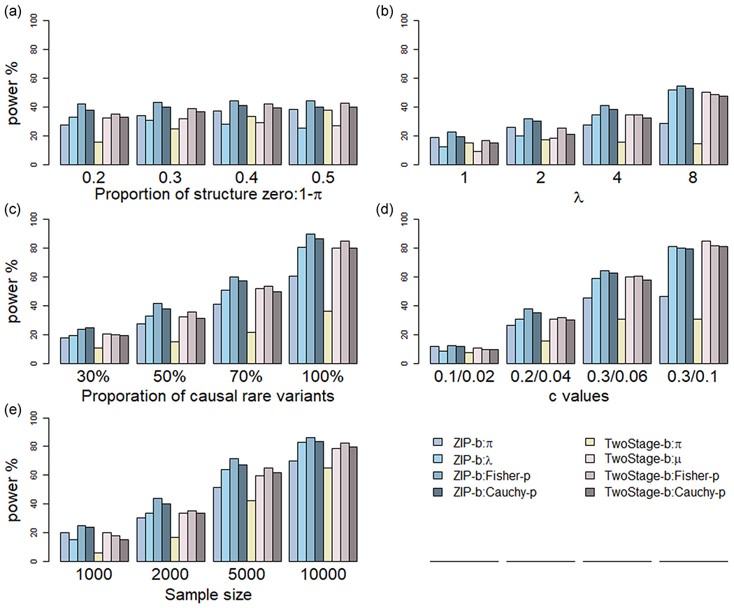
Power comparisons of ZIP-b and two-stage burden tests on zero-inflated count data. Power was estimated under the following parameter settings: (a) proportion of structural zero (1 − π: 0.2, 0.3, 0.4, 0.5), (b) average count from the Poisson distribution (λ: 1, 2, 4, 8), (c) proportion of rare variants to be causal (30%, 50%, 70%, 100%), (d) genetic magnitude of γπ and γλ: cπ/cλ values (0.1/0.02, 0.2/0.04, 0.3/0.06, 0.3/0.1), and (e) sample size (1000; 2000; 5000; 10,000); variant weight wB = Beta(p; 1, 25) where p is the population MAF. ZIP-b: ZIP burden test; TwoStage-b: two-stage burden test
FIGURE 2.
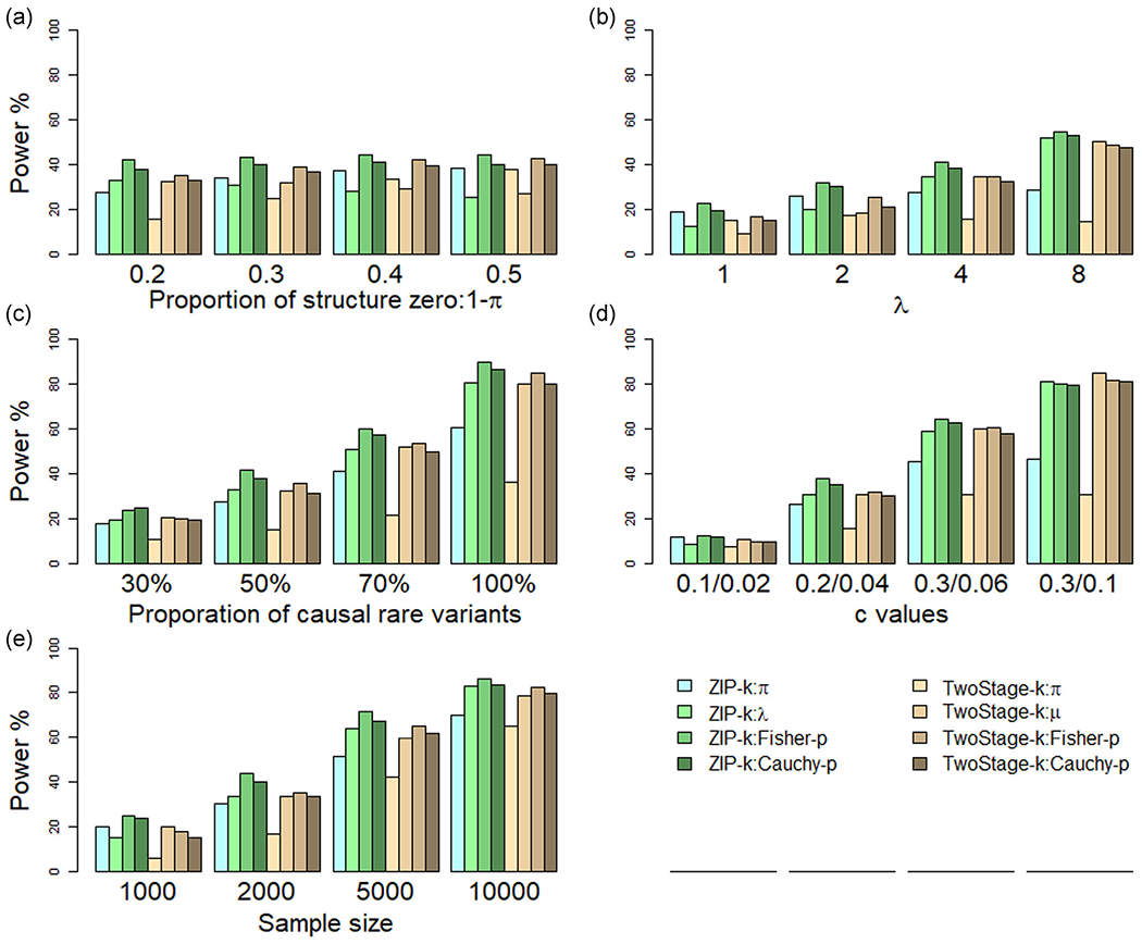
Power comparisons of ZIP-k and two-stage kernel tests on zero-inflated count data. Power was estimated under the following parameter settings: (a) proportion of structural zero (1 − π: 0.2, 0.3, 0.4, 0.5), (b) average counts from the Poisson distribution (λ: 1, 2, 4, 8), (c) proportion of rare variants to be causal (30%, 50%, 70%, 100%), (d) genetic magnitude of γπ and γλ: cπ/cλ values (0.1/0.02, 0.2/0.04, 0.3/0.06, 0.3/0.1), and (e) sample size (1000; 2000; 5000; 10,000); variant weighting wB = Beta(p; 1, 25) where p is the population MAF. ZIP-k: ZIP kernel test; TwoStage-b: two-stage kernel test
For testing the effects of individual parameters γπ and γλ, as well as the omnibus test using Fisher-p and Cauchy-p methods, the proposed ZIP-b consistently outperformed ZIP-k in all scenarios when all variants had the same direction of the effect on the phenotype, as shown in Figures 1 and 2. For example, as structured zeros from 0.2 to 0.5, the power to test γπ ranged from 0.394 to 0.515 for ZIP-b, whereas 0.279 to 0.384 for ZIP-k. We also observed that, for global tests, Fisher’s method slightly outperformed Cauchy’s method. For the same scenario above, for instance, Fisher-p yielded power from 0.593 to 0.618 whereas Cauchy-p from 0.550 to 0.564 for ZIP-b, with a similar trend for ZIP-k (0.420 to 0.443 vs. 0.380 to 0.411 for Fisher’s and Cauchy’s methods, respectively). This could be explained partially that the association signals were attributed to both parameters in the simulation settings, whereas the Cauchy-p method is most effective when the signal was from a single parameter (Liu & Xie, 2020).
As compared with the two-stage approach, first, we examined the scenarios in which all causal variants had consonant effects, that is, the direction of effects was the same in γπ and γλ (Figures 1& and 2). For the genetic association testing on γπ, the ZIP-b and ZIP-k approaches particularly showed superior statistical power than the two-stage burden and kernel tests accordingly on . For instance, for the burden test, ZIP γπ testing had a power of 0.351, in contrast to 0.257 for the two-stage , given 50% variants were causal, and 0.884 versus 0.752 given 100% causal variants. Notably, the power was comparable for testing γλ from our method and γμ from the two-stage approach. Secondly, we sought to compare the omnibus test on γπ and γλ (or and γμ for the two-stage test) using Fisher-p and Cauchy-p methods. Our omnibus test outperformed the two-stage test across all the simulated settings. For instance, for burden test at varying λ, ZIP Fisher’s method yielded power from 0.300 to 0.708 whereas the two-stage approach had power from 0.218 to 0.669, with a similar trend for Cauchy’s method (0.240 to 0.684 vs. 0.214 to 0.639 for ZIP and two-stage methods, respectively)
When causal variants had mixed direction of effects, that is, the effect directions of γπ and γλ were 50% positive and 50% negative (i.e., 50%+; Figure 3), 40% positive and 60% positive (Figure S2), the ZIP-k test outperformed the ZIP-b test. However, when there was a small proportion of the opposite direction of effects, that is, the majority was positive at 80%, the ZIP-k had similar power with the ZIP-b test. Compared with the two-stage method, ZIP-b and ZIP-k tests had similar power in certain settings (i.e., positive at 80% and negative at 20%); but this did not carry through to other settings (i.e., positive at 50% and negative at 50%), whereas the two-stage had power gain.
FIGURE 3.

Power of testing procedures for variants having consonant or dissonant effects in different directions. The effect directions for γπ and γλ are either 100% positive (0% negative; denoted as 100/0 in the figure) and 50% positive (50% negative; 50/50). The plots consider both consonant and dissonant settings. For the consonant setting, the effect direction of γπ and γλ are the same; while for dissonant setting, the direction of γπ and γλ are opposite. Results from the burden tests are in the upper panel, and kernel tests in the lower panel. TwoStage-b, two-stage burden test; TwoStage-k: two-stage kernel test; ZIP-b, ZIP burden test; ZIP-k, ZIP kernel test
Further, we evaluated the dissonant setting in which the genetic directions of γπ and γλ were opposite (Figure 3). Similarly, we observed that the ZIP model outperformed the two-stage for testing γπ and omnibus tests. For example, for the global test when directions of γπ were all positive and γλ all negative (100/0; the right panel of Figure 3), Fisher’s method on ZIP burden test had the power of 0.480, in contrast to 0.446 for the two-stage method, and similarly for kernel test (0.389 vs. 0.302 for ZIP and two-stage methods, respectively). When causal variants had mixed directions of effects, both ZIP and two-stage kernel tests outperformed their counterparts—burden tests.
The variant weighting scheme wB = Beta(p, 1, 25) was used in the above power comparison, where p is the population MAF. We also conducted power calculation using other variant weighting schemes: w0 = 1 and , where is the sample MAF estimate. We observed that the power estimates among these three variant weighting schemes were negligible for all simulation settings (Figures S3–S6). The findings held for both ZIP-b and ZIP-k methods. In all settings under investigation, our proposed approach outperformed or comparable with the two-stage method.
For the scenarios when we restricted to ultra-rare variants (MAF <0.001) only, ZIP-b outperformed the two-stage method burden tests for different sample sizes from 1000 to 10,000, whereas ZIP-k had comparable power with the two-stage methods at a large sample size, that is, 10,000 (Figure S7). Clearly, the degree of statistical power is highly related to sample sizes. When ultra-rare variants were included, larger sample sizes are needed, particularly, for kernel-based tests. For the sensitivity analyses using uniform distribution to define variant effect sizes, the statistical power of the ZIP methods outperformed that of the two-stage approach for both burden and kernel, and omnibus tests (Figure S8), similar pattern as observed in Figures 1 and 2. Within each method (ZIP-b or ZIP-k), we also noted that a slightly higher power for the effect sizes drawn from the uniform distribution, than those defined by the inversely proportional to the population MAF of each variant.
3.3 |. Application to ROSMAP data
Using WGS data in 1149 individuals from the ROSMAP study, we tested whether there were associations between rare variants and neuritic plaques in brain for 25 genes reported in a recent large-scale GWAS for Alzheimer’s disease risk (Kunkle et al., 2019). The zero counts accounted for 28.9% of the total samples and the average count was 11.8. The medium counts of rare variants in each gene were . We examined the results using our proposed method and the two-stage method using “SKAT” package in R. There were six genes showing marginal signals from either or both methods at p-values less than 0.05 for testing γπ, γλ, or γμ when all rare variants were included, and four genes when rare variants restricted to LOF variants (Table 3).
TABLE 3.
Analysis of the rare variant effects on neuritic plaques in ROSMAP sequencing data
| ZIP-b |
ZIP-k |
TwoStage-b |
TwoStage-k |
ZIP-b |
ZIP-k |
TwoStage-b |
TwoStage-k |
||||||||||
|---|---|---|---|---|---|---|---|---|---|---|---|---|---|---|---|---|---|
| Gene | Var. no. | π | λ | π | λ | π′ | μ | π′ | μ | Fisher-p | Cauchy-p | Fisher-p | Cauchy-p | Fisher-p | Cauchy-p | Fisher-p | Cauchy-p |
| rare var. | |||||||||||||||||
| ADAM10 | 630 | 0.516 | 0.478 | 0.020 | 0.536 | 0.472 | 0.203 | 0.094 | 0.178 | 0.592 | 0.497 | 0.059 | 0.040 | 0.320 | 0.301 | 0.085 | 0.123 |
| ACE | 93 | 0.774 | 0.007 | 0.530 | 0.047 | 0.749 | 0.020 | 0.527 | 0.095 | 0.036 | 0.015 | 0.116 | 0.093 | 0.076 | 0.041 | 0.199 | 0.179 |
| CASS4 | 170 | 0.576 | 0.322 | 0.336 | 0.032 | 0.435 | 0.043 | 0.264 | 0.055 | 0.498 | 0.440 | 0.059 | 0.060 | 0.094 | 0.083 | 0.076 | 0.093 |
| CR1 | 492 | 0.250 | 0.135 | 0.564 | 0.047 | 0.153 | 0.021 | 0.513 | 0.001 | 0.148 | 0.177 | 0.123 | 0.095 | 0.022 | 0.038 | 0.004 | 0.002 |
| SLC24A4 | 747 | 0.817 | 0.460 | 0.800 | 0.095 | 0.694 | 0.322 | 0.670 | 0.013 | 0.744 | 0.697 | 0.272 | 0.261 | 0.558 | 0.511 | 0.050 | 0.027 |
| SORL1 | 660 | 0.179 | 0.669 | 0.654 | 0.213 | 0.025 | 0.395 | 0.505 | 0.068 | 0.374 | 0.352 | 0.414 | 0.388 | 0.055 | 0.048 | 0.149 | 0.130 |
|
| |||||||||||||||||
| LOF var. | |||||||||||||||||
| FERMT2 | 3 | 0.001 | 0.151 | 0.004 | 0.262 | 0.029 | 0.060 | 0.075 | 0.118 | 0.001 | 0.002 | 0.008 | 0.008 | 0.013 | 0.039 | 0.051 | 0.092 |
| NYAP1 | 8 | 0.002 | 0.758 | 0.066 | 0.709 | 0.012 | 0.431 | 0.173 | 0.441 | 0.012 | 0.004 | 0.189 | 0.147 | 0.033 | 0.024 | 0.272 | 0.263 |
| PTK2B | 8 | 0.559 | 0.159 | 0.473 | 0.413 | 0.610 | 0.049 | 0.531 | 0.344 | 0.305 | 0.281 | 0.515 | 0.443 | 0.134 | 0.101 | 0.493 | 0.432 |
| SORL1 | 15 | 0.049 | 0.404 | 0.069 | 0.304 | 0.031 | 0.513 | 0.036 | 0.231 | 0.098 | 0.092 | 0.103 | 0.117 | 0.082 | 0.062 | 0.049 | 0.064 |
Note: Analyses included the individual burden and kernel tests on γπ and γλ from the ZIP-b and ZIP-k methods, and , and γμ from the two-stage approach, as well as omnibus tests using Fisher-p and Cauchy-p. The upper table shows the results from the analysis on rare variants in each gene (MAF <0.002), and the lower table only for a subset of lost-of-function (LOF) rare variants. The genes with p-value <0.05 for any individual test are listed here. The smallest p-value from either individual tests or omnibus tests are italicized for each gene. Variant weight wB = Beta(p; 1, 25) where p is the population MAF.
Abbreviations: TwoStage-b, two-stage burden test; TwoStage-k, two-stage kernel test; ZIP-b, ZIP burden test; ZIP-k, ZIP kernel.
Under the scenario of using all rare variants in the gene, for individual parameter tests, three genes ACE, CASS4, and CR1 were detected by both ZIP and two-stage methods, where ZIP methods showed more significant than the two-stage method (P = 0.007 vs. P = 0.020 for ACE for testing γλ or γμ). Of these genes, the association with neuritic plaques data was mainly attributed to the effects on the average counts or non-zero counts (testing for ZIP γλ or two-stage γμ). Gene ADAM10 was detected by ZIP only (P = 0.02), but borderline signal was also found by the two-stage method (P = 0.09). However, opposite pattern was found in SLC24A4 and SORL1, which were detected by the two-stage method but borderline or no signals in ZIP method (e.g., P = 0.013 vs. P = 0.095 for SLC24A4 for testing γμ or γλ). For the omnibus tests, in general, Cauchy’s method yielded comparable or slightly smaller p-value in contrast to Fisher’s method. Not surprisingly, given the moderate sample size of the ROSMAP data, the majority of genes under examination did not show any associations between the rare variants and neuritic plaque counts using both methods. For the analyses using filtered only LOF variants, three genes of FERMT2, NYAP1 and SORL1 were detected by both methods (Table 3). For FERMT2 and NYAP1, ZIP methods showed much stronger significance than the two-stage methods (FERMT2: P = 0.001 vs. P = 0.029 for testing γπ and ; NYAP1: P = 0.002 vs. P = 0.012 for testing γπ and ). Gene SORL1 was the same one detected above using all rare variants, but with more tests showing significant signals. Under this rare variant selection setting, both two-stage burden and kernel tests detected (P = 0.031 and 0.036), and ZIP-b detected γπ (P = 0.049) for SORL1. Here we used variant weighting wB = Beta(p, 1, 25), whereas the results were similar if no weighting schemes were applied to variants (Table S3).
4 |. DISCUSSION
We have proposed novel ZIP-b and ZIP-k methods to test the association between a group of rare variants and zero-inflated counts. Our methods are slightly outperformed the two-stage test, whereas adequately controlling type 1 error, in the simulation scenarios we considered; the power gain is more evident for testing the structure zeros. On the other hand, ZIP-b outperformed ZIP-k in all settings except that both deleterious and protective variants coexisted in a gene (i.e., the directions of genetic effects were mixed). In such a scenario, ZIP-k was comparable to the two-stage kernel test. We also illustrated the usages of ZIP methods by analyzing AD candidate genes for the neuritic plaques from the ROSMAP study. We showed rare variants in six AD risk genes potentially associated with neuritic plaque counts.
Currently, for the zero-inflated count data, there is no integrated modeling to analyze the effects of a set of rare variants on the structure zero and count data simultaneously. The most common approach in practice is the two-stage approach. Assume the count zero representing subjects without the disease and the non-zero count representing disease severity. The two-stage test models the disease status and disease severity separately. However, it compromised in the appropriate layout of the testing statistics. First, the estimated 1-π′ is not for the structured zeros, but instead the proportion of the observed zeros. Second, μ is misspecified as zero-truncated Poisson counts. Thus, the individual test on π′ and μ is only analogous to test parameters π and λ from the mixed Binomial and Poisson distribution for ZIP data. Our method accurately tests the underlying two components of the zero-inflated count data, with the increased power for both individual and the omnibus test. For example, in the application to ROSMAP data, ZIP-k detected a significant association between rare variants in ADAM10 and structured zeros of neuritic plaques counts (p = 0.020). However, the two-stage approach could be biased as binominal distribution was shifted by modeling observed zeros, instead of structured zeros, which may explain the borderline result (p = 0.094). Besides, our method also outperformed in the scenarios of dissonant effects, where a set of variants increased the likelihood of structure zeros, while at the same time increased the mean of the counts. There is one setting that the two-stage method outperformed slightly than our proposed method in the presence of a mixture of directions in the genetic effects, that is, the direction of genetic effect 80% positive and 20% negative. However, this did not carry on to scenarios at other varying proportions whereas our method slightly outperformed or was comparable to the two-stage approach.
With the large-scale sequencing data becoming available to public, such as the population-based UK Biobank data, precisely modeling the distribution of phenotype has the potential to increase the power of association tests (Bi et al., 2021). Our method can be applied to analyze on the rare and ultra-rare variants for various zero-inflated counts, such as hospitalization episode derived from the Electronic medical records (EMRs) in general population (Bycroft et al., 2018), drusen measures of counts for macular degeneration patients (Chavali et al., 2015), and counts data for hand osteoarthritis(Boer et al., 2021). Further, the presence of excessive zero counts is the inherent feature of microbiome count data (Kaul et al., 2017). Our methods will be applicable to these data if one wants to investigate the association between a set of rare variants with such microbiome counts. As the score test is generally easier to compute, the proposed method is computationally efficient in both simulation and real data analyses. The R programs for both ZIP-b and ZIP-k tests will be available for researchers to use in the future.
Although the type I error is generally controlled for both ZIP-b and ZIP-k tests in all simulation setting with no variant weight or Beta variant weight applied, ZIP-k tends to have slightly lower type I errors comparing to ZIP-b. This is similar to what we observed in our previous study of gene-based methods for the censored trait (Qi et al., 2019). These small deflation in kernel-based tests could be potentially due to the use of Davies’ method (Davies, 1980) in approximating a mixture of two distributions to obtain p-values efficiently. However, we observed extreme deflation of type I errors in ZIP-K when Madsen and Browning’s variant weighting was used. Although it is consistent to what we previously observed in Qi et al. (2019), this deflation problem might be due to other reasons beyond the use of Davies’ method, which warrants further investigations. As of now, we would not recommend using the Madsen and Browning variant weight in our proposed ZIP gene-based association tests. In addition, our evaluation on the impacts of small sample sizes suggested that we should be cautious to apply ZIP methods when sample sizes are less than 1000 due to the inflated type I error rates. However, this may not be a big concern in the application as a large-scale sequencing data is a current trend.
In this study, we applied three methods to combine tests for π and λ: Fisher-p, Cauchy-p and Min-p methods. The Min-p method was incapable to control type 1 error thus we omitted it from the power calculation. For the power estimation, Fisher-p had greater power than Cauchy-p in various simulation settings we considered. However, Cauchy-p was slight smaller compared with Fisher-p using ROSMAP data. This could be explained by the different properties of these two tests. It is known that Cauchy-p is most effective when there is only one or a few significant p-values regardless of others, that is, if the majority p-values are not significant, Cauchy-p is expected to be most effective (Liu & Xie, 2020). On the other hand, Fisher-p could be more suitable in combining of p-values when the association signals were attributed from both parameters.
Our proposed ZIP-b and ZIP-k methods can be extended in various ways to accommodate the more complex data structure. For example, we can extend our method to have joint statistics for both common and rare variants accounting for the linkage disequilibrium. Also, our ZIP framework can be extended to account for the potential dispersion or heterogeneity in the data. In case when the over-dispersion is a significant problem of the phenotype, modeling the outcome as the Zero-Inflated Negative Binomial (ZINB) distribution, rather than the ZIP distribution, is regarded as a more robust approach for association testing (Mallick & Tiwari, 2016; Yu et al., 2013). It is unclear whether this could be a similar pattern for rare variants, and what scenario is applicable for switching to ZINB model. Further development on extending our proposed framework based on ZINB distribution for the zero-inflated outcomes will be an interesting topic for the future study.
Supplementary Material
ACKNOWLEDGMENTS
This study was supported by National Institute of Aging (NIA) of National Institutes of Health (NIH) grant R01 AG060472, and Singapore Ministry of Health (MOE) grant R-317-000-138-115. We thank the study participants and staff of the Rush Alzheimer’s Disease Center (RADC), Rush University Medical Center for the ROSMAP cohort. ROSMAP resources can be requested at https://www.radc.rush.edu. The ROSMAP work was supported by NIA grants to the RADC including the Religious Orders Study (P30AG010161, R01AG015819), the Rush Memory and Aging Project (R01AG017917), AMP-AD Pipeline I (U01AG46152) and AMP-AD Pipeline II (U01AG61356).
Footnotes
SUPPORTING INFORMATION
Additional supporting information may be found in the online version of the article at the publisher’s website.
REFERENCES
- Beecham GW, Hamilton K, Naj AC, Martin ER, Huentelman M, Myers AJ, Corneveaux JJ, Hardy J, Vonsattel J-P, Younkin SG, Bennett DA, De Jager P, Larson EB, Crane PK, Kamboh MI, Buxbaum JD, Kramer P, Dickson DW, Farrer LA, … Montine TJ (2014). Genome-wide association meta-analysis of neuropathologic features of alzheimer’s disease and related dementias. PLoS Genetics, 10(9):e1004606. [DOI] [PMC free article] [PubMed] [Google Scholar]
- Bennett DA, Buchman AS, Boyle PA, Barnes LL, Wilson RS, & Schneider JA (2018). Religious orders study and rush memory and aging project. Journal of Alzheimer’s Disease, 64(s1), S161–S189. [DOI] [PMC free article] [PubMed] [Google Scholar]
- Bi W, Zhou W, Dey R, Mukherjee B, Sampson JN, & Lee S (2021). Efficient mixed model approach for large-scale genome-wide association studies of ordinal categorical phenotypes. The American Journal of Human Genetics, 108(5), 825–839. [DOI] [PMC free article] [PubMed] [Google Scholar]
- Boer CG, Yau MS, Rice SJ, de Almeida RC, Cheung K, Styrkarsdottir U, Southam L, Broer L, Wilkinson JM, Uitterlinden AG, Zeggini E, Felson D, Loughlin J, Young M, Capellini TD, Meulenbelt I, & van Meurs JB (2021). Genome-wide association of phenotypes based on clustering patterns of hand osteoarthritis identify WNT9A as novel osteoarthritis gene. Annals of the Rheumatic Diseases, 80(3), 367–375. [DOI] [PMC free article] [PubMed] [Google Scholar]
- Bycroft C, Freeman C, Petkova D, Band G, Elliott LT, Sharp K, Motyer A, Vukcevic D, Delaneau O, O’Connell J, Cortes A, Welsh S, Young A, Effingham M, McVean G, Leslie S, Allen N, Donnelly P, & Marchini J (2018). The UK Biobank resource with deep phenotyping and genomic data. Nature, 562(7126), 203–209. [DOI] [PMC free article] [PubMed] [Google Scholar]
- Chavali VRM, Diniz B, Huang J, Ying G-S, Sadda SR, & Stambolian D (2015). Association of OCT-derived drusen measurements with AMD-associated genotypic SNPs in the Amish population. Journal of Clinical Medicine, 4(2), 304–317. [DOI] [PMC free article] [PubMed] [Google Scholar]
- Davies RB (1980). The distribution of a linear combination of χ2 random variables. Applied Statistics, 29(3), 323–333. [Google Scholar]
- Famoye F, & Singh KP (2006). Zero-inflated generalized Poisson regression model with an application to domestic violence data. Journal of Data Science, 4(1), 117–130. https://jds-online.org/journal/JDS/article/1054/info [Google Scholar]
- Goodman MO, Chibnik L, & Cai T (2019). Variance components genetic association test for zero-inflated count outcomes. Genetic Epidemiology, 43(1), 82–101. [DOI] [PMC free article] [PubMed] [Google Scholar]
- Gupta PL, Gupta RC, & Tripathi RC (2005). Score test for zero inflated generalized Poisson regression model. Communications in Statistics—Theory and Methods, 33(1), 47–64. 10.1081/STA-120026576 [DOI] [Google Scholar]
- Jansakul N, & Hinde J (2002). Score tests for zero-inflated Poisson models. Computational Statistics & Data Analysis, 40(1), 75–96. [Google Scholar]
- Jiang Y, Ji Y, Sibley AB, Li YJ, & Allen AS (2017). Leveraging population information in family-based rare variant association analyses of quantitative traits. Genetic Epidemiology, 41(2), 98–107. [DOI] [PubMed] [Google Scholar]
- Jung J, Dantzer J & Liu Y (2011). Identification of multiple rare variants associated with a disease. In Ghosh S, Bickeböller H, Bailey J, Bailey-Wilson JE, Cantor R, Daw W, DeStefano AL, Engelman CD, Hinrichs A, Houwing-Duistermaat J, König IR, Kent J, Pankratz N, Paterson A, Pugh E, Sun Y, Thomas A, Tintle N, Zhu X, MacCluer JW, & Almasy L (Eds.), BMC Proceedings 5, S103. Springer. [DOI] [PMC free article] [PubMed] [Google Scholar]
- Kaul A, Mandal S, Davidov O, & Peddada SD (2017). Analysis of microbiome data in the presence of excess zeros. Frontiers in Microbiology, 8, 2114. [DOI] [PMC free article] [PubMed] [Google Scholar]
- Kunkle BW, Grenier-Boley B, Sims R, Bis JC, Damotte V, Naj AC, Boland A, Vronskaya M, Van Der Lee SJ, Amlie-Wolf A, Bellenguez C, Frizatti A, Chouraki V, Martin ER, Sleegers K, Badarinarayan N, Jakobsdottir J, Hamilton-Nelson KL, Moreno-Grau S… Pericak-Vance MA (2019). Genetic meta-analysis of diagnosed Alzheimer’s disease identifies new risk loci and implicates a β, tau, immunity and lipid processing. Nature Genetics, 51(3), 414–430. [DOI] [PMC free article] [PubMed] [Google Scholar]
- Lambert D (1992). Zero-inflated Poisson regression, with an application to defects in manufacturing. Technometrics, 34(1), 1–14. [Google Scholar]
- Lee AH, Wang K, Scott JA, Yau KK, & McLachlan GJ (2006). Multi-level zero-inflated Poisson regression modelling of correlated count data with excess zeros. Statistical Methods in Medical Research, 15(1), 47–61. [DOI] [PubMed] [Google Scholar]
- Li B, & Leal SM (2008). Methods for detecting associations with rare variants for common diseases: Application to analysis of sequence data. American Journal of Human Genetics, 83(3), 311–321. [DOI] [PMC free article] [PubMed] [Google Scholar]
- Liu Y, & Xie J (2020). Cauchy combination test: A powerful test with analytic p-value calculation under arbitrary dependency structures. Journal of the American Statistical Association, 115(529), 393–402. [DOI] [PMC free article] [PubMed] [Google Scholar]
- Madsen BE, & Browning SR (2009). A groupwise association test for rare mutations using a weighted sum statistic. PLoS Genetics, 5(2), e1000384. [DOI] [PMC free article] [PubMed] [Google Scholar]
- Mallick H, & Tiwari HK (2016). EM adaptive LASSO—A multilocus modeling strategy for detecting SNPs associated with zero-inflated count phenotypes. Frontiers in Genetics, 7, 32. [DOI] [PMC free article] [PubMed] [Google Scholar]
- Morris AP, & Zeggini E (2010). An evaluation of statistical approaches to rare variant analysis in genetic association studies. Genetic Epidemiology, 34(2), 188–193. [DOI] [PMC free article] [PubMed] [Google Scholar]
- Neale BM, Rivas MA, Voight BF, Altshuler D, Devlin B, Orho-Melander M, Kathiresan S, Purcell SM, Roeder K, & Daly MJ (2011). Testing for an unusual distribution of rare variants. PLoS Genetics, 7(3), e1001322. [DOI] [PMC free article] [PubMed] [Google Scholar]
- Patterson N, Price AL, & Reich D (2006). Population structure and eigenanalysis. PLoS Genetics, 2(12), e190. [DOI] [PMC free article] [PubMed] [Google Scholar]
- Qi W, Allen AS, & Li Y-J (2019). Family-based association tests for rare variants with censored traits. PloS One, 14(1), e0210870. [DOI] [PMC free article] [PubMed] [Google Scholar]
- Schaffner SF, Foo C, Gabriel S, Reich D, Daly MJ, & Altshuler D (2005). Calibrating a coalescent simulation of human genome sequence variation. Genome Research, 15(11), 1576–1583. [DOI] [PMC free article] [PubMed] [Google Scholar]
- Vilor-Tejedor N, Alemany S, Forns J, Cáceres A, Murcia M, Marià D, Pujol J, Sunyer J, & González J (2019). Assessment of susceptibility risk factors for ADHD in imaging genetic studies. Journal of Attention Disorders, 23(7), 671–681. [DOI] [PubMed] [Google Scholar]
- Wu MC, Lee S, Cai T, Li Y, Boehnke M, & Lin X (2011). Rare-variant association testing for sequencing data with the sequence kernel association test. American Journal of Human Genetics, 89(1), 82–93. [DOI] [PMC free article] [PubMed] [Google Scholar]
- Yan A, Laird NM, & Li C (2011). Identifying rare variants using a Bayesian regression approach. In BMC Proceedings (Vol. 5, pp. 1–5). Springer. [DOI] [PMC free article] [PubMed] [Google Scholar]
- Yu D, Huber W, & Vitek O (2013). Shrinkage estimation of dispersion in negative binomial models for RNA-seq experiments with small sample size. Bioinformatics, 29(10), 1275–1282. [DOI] [PMC free article] [PubMed] [Google Scholar]
Associated Data
This section collects any data citations, data availability statements, or supplementary materials included in this article.