Abstract
This paper investigates the effects of the pandemic containment periods in France on individuals’ movements, expenditure and adaptation to the shock, using billions of French bank card transactions measured before and during the COVID-19 pandemic. We measure not only the effect on consumer expenditure, but also on quantities directly related to the containment restrictions, such as consumer mobility, number of retailers visited, and inter-regional purchases. The results show large effects on these measures of consumers’ movements, as well as on both online and offline measures of expenditure, particularly in the first containment period. We also find evidence that consumers adjusted rapidly during the first containment period, mitigating the effects of mobility restrictions via an increasing shift toward online purchasing, and that the nature of the adaptation differed for different types of purchase.
Keywords: COVID-19, Consumer mobility, Consumption expenditure, Containment policy, Inter-regional trade, Transaction data
1. Introduction
In response to the coronavirus pandemic which began in 2019–20, governments throughout the world introduced policies designed to contain the virus through restrictions on interactions among individuals. In addition to the intended effects on spread of the virus, there were inevitable effects of these policies on economic activity. Many of these effects, both epidemiological and economic, were expected to operate through the channel of reduced individual interaction and movement, as well as through the closure of businesses and public places.
The goal of this paper is to study these effects, using an exceptionally rich and detailed data set of French consumer transactions. The study of individuals’ movements is critical for this purpose. While other data sources can give indications of effects on consumption, the precise time and location information in these data allow us, in addition to tracing dynamic economic effects at a fine level of detail, to characterize changes in consumer mobility resulting from the combination of the pandemic and policy responses at a level of detail which was not possible prior to the era of high-frequency consumer data.
We address a number of distinct research questions. First, in common with a number of recent studies using data from different countries, we examine the degree to which consumer expenditure was reduced, at each point in time, through the pandemic and the first two containment periods in 2020, which were the most severe in France. The coverage and precision of the data that we use are well adapted to this dynamic tracking, as well as to describing expenditure patterns at time scales as fine as each hour within the day, and we do so here. However, we also consider a number of more subtle questions.
The direct impact of the containment policy was on the movements of consumers, whether within their own cities, to businesses, or to regions outside. These restrictions on consumer movement, along with restrictions on the opening of retail outlets, formed a part of the set of factors contributing to the reduction in consumption. The data that we use, containing as they do a precise geographical location for each transaction, allow us to measure directly the reduction in consumer mobility. In particular, we track changes in the distributions across consumers of total distance travelled, number of cities or regions visited, and number of retailers visited.
The data also contain information about whether a purchase was made on-site or online. The restrictions on movement of consumers to physical stores, or the policy restrictions on the opening of physical stores, might be expected to increase the relative attractiveness of online purchases and to encourage consumers to adapt to the shock conditions by shifting some of their purchases in that direction. We are able to measure the degree to which such substitution of online for on-site purchasing took place through the period of the containment. Such substitution may not only imply greater resilience to the shock, but may lead to long-lasting changes in consumer behaviour resulting from learning.
A further aim of this paper is to describe this consumer adaptation, including some indication of the speed at which it took place, within the limitations imposed by the time span of the data. Because there were two separate periods of containment during the period under study, which were similar with respect to consumer mobility restrictions, we are able to draw some inferences about consumer learning and adaptation, and the degree to which the adaptations had durable effects, by comparison of these periods with each other as well as with the pre-pandemic period.
The reduction in physical mobility of consumers also has implications for economic activity in different regions of France. Different regions are affected to different degrees by restrictions on the ability of consumers from other regions to visit, and we therefore expect not only that purchases by consumers exterior to their own regions will be reduced, but that different regions will suffer differing degrees of economic loss. The information in our data allows us to identify the locations of different transactions, and to impute a home location to each card holder, allowing us to measure external transactions and therefore measure the degree to which these were curtailed.
To address the various research questions, we rely on detailed bank card transaction data from billions of French consumer transactions, before and during the shock induced by COVID-19. The data set that we exploit is one of the richest data sets that has been made available to researchers, consisting of the set of transactions made on millions of bank cards in France in the years 2019 and 2020, and covering two separate periods of containment, totalling nearly 20 billion transactions.1 The information on timing and location of the transaction, and nature of the merchant, allows us to draw conclusions at a finely detailed level; in particular, the location information permits us to analyse changes in consumer mobility by measuring distances between successive purchases in different locations. As well, the nearly 20 billion transactions that we track were made via over 60 million cards payment cards, issued by all banks in France; we therefore avoid the potential for bias arising from the use of data from specialized means of payment which may be used by a small or unrepresentative fraction of the general population.
We are able to establish a number of results concerning the extent of the reduction in individuals’ movements, which was a key mechanism by which containment policies were intended to reduce the spread of infection. Consumers’ mobility was substantially reduced during the containment periods, particularly during the first period: cards travelled on average one-third of the total distance during the first containment period in 2020 compared with the same period in 2019, visited fewer cities (35% of cards were used in a single city compared with 12% in 2019), spent more in the home city (36% of transactions by value are recorded in the home city during this period versus 12% in 2019), and purchases were concentrated on a smaller number of retailers.
We estimate strongly significant declines in both value and volume (41% and 50% respectively) during the first containment period, and a strongly significant increase in average transaction volume (17%), consistent with fewer shopping trips but a greater value of purchases in each; we observe that the overall decline in consumer spending is significantly greater at the end of the day, at the end of the week, and in physical stores (compared with online). We also note that consumers responded strongly to announcement of the containment policy’s restrictions, first with some anticipatory purchases – the total transaction value increased by almost 40% on the last day before the containment period, March 16 – and second by a dramatic drop in the first days of containment, of around −60%, before gradually beginning to recover. The overall decline in point-of-sale (POS) expenditure was approximately twice as great as the decline in online expenditure, and while the drop in POS spending stabilized around −40% at the end of the first containment period, online spending had already returned to its pre-pandemic level. However, effects observed during the second containment period were smaller, a point which we discuss below in the context of consumer adaptation.
With respect to purchases made by consumers from other regions of France (‘inter-regional expenditures’), we find large declines during both containment periods, and indeed throughout the part of the pandemic period in our sample, in all measures of monthly inter-regional consumer purchases (value, volume, number of cards making an external purchase, and number of retailers from which a purchase was made), relative to the counterfactual path without the COVID-19 outbreak event.
This paper is one of several recent studies that investigate the effects of the Covid-19 pandemic. We treat aspects of both consumers’ expenditure and mobility, and so the present study is related to a large literature on household expenditure (see among others Souleles, 1999, Johnson et al., 2006, Agarwal et al., 2007, Agarwal and Qian, 2014, Kaplan and Violante, 2014, Di Maggio et al., 2017, Baker, 2018), to a recent literature on consumer mobility (Agarwal et al., 2019a, Bounie et al., 2020b), as well as to the growing recent literature on the economic consequences of COVID-19 that spans macroeconomic perspectives (Atkeson, 2020a, Piguillem and Shi, 2020, Guerrieri et al., 2020, Eichenbaum et al., 2020, McKibbin and Roshen, 2020), financial markets (Alfaro et al., 2020, Baker et al., 2020a), labour markets (Alon et al., 2020, Dingel and Neiman, 2020), health (Kuchler et al., 2020, Atkeson, 2020b), social distancing (Jones et al., 2020, Chiou and Tucker, 2020), and firms and households.2 The present study emphasizes the behaviour of individuals, rather than of firms.
Chen et al. (2020) use daily transaction data in 214 cities to study the impact of COVID-19 on consumption after China’s outbreak in late January 2020. China was the first country to experience a large-scale outbreak, and the first country to implement drastic measures to contain the spread, e.g. lockdown, social distancing, tracing, and closure of non-essential activities. The authors use transaction data from one of China’s largest payment service providers, UnionPay, which covers around 30% of China’s total retail consumption off-line. Using difference-in-differences regressions to estimate effects on daily off-line consumption, they find that heavily exposed cities, such as Wuhan, saw their off-line consumption reduced by close to 70% during a twelve-week period, and infer that China’s 2019 GDP decreased by 1.2%. Carvalho et al. (2021) also use transaction data, from BBVA, the second-largest bank in Spain, to analyse the dynamics of expenditure during the ongoing COVID-19 pandemic. They find a significant reduction of about 49% in aggregate expenditure when compared with the same period in 2019. They also find sectoral and regional variations in expenditure change in the data, and that off-line expenditure declined substantially more than the online expenditure after the national lockdown. Andersen et al. (2020) is another study that uses transaction-level customer data, from the largest bank in Denmark; Denmark experienced a partial shutdown of economic activity, less restrictive than in Spain for instance. This study finds that aggregate card spending dropped by around 25% following the shutdown. The drop is mostly concentrated in restricted goods and services, and is larger for individuals more exposed to the economic and health risks introduced by the COVID-19 crisis. Finally, Baker et al. (2020b) use a sample of several hundred thousand transactions made by 4735 US consumers who hold accounts with a non-profit Fintech company that works with individuals to sustain savings habits. They find that initially spending increased sharply, particularly in retail, credit card spending and food items, and was followed by a sharp decrease in overall spending. Households responded most strongly in states with shelter-in-place orders.
One respect in which the present research differs from those just cited is that we analyse the payment card data of the general domestic card payment scheme in France, and thus from the customers of all French banks, rather than from a single major bank. We therefore expect excellent coverage of French consumers and of the effects of the crisis throughout the country. However, it is important also to acknowledge several limitations of the analysis that we are able to perform. First, we emphasize that we estimate effects of a set of approximately simultaneous conditions on consumer behaviour: the dates of periods of containment were endogenous to infection rates, and these periods were therefore times not only of policy restriction, but also of heightened concern in the population. We estimate effects on consumer expenditure and mobility of this set of conditions, not of policy restrictions alone. Second, our data contain card transactions only. While these data are highly informative concerning these card transactions, containing both debit and credit expenditures, we do not measure cash transactions. While we might expect cash transactions to have been reduced to a degree similar to the reduction in in-store card purchases during the containment periods, these are not measured.3
The rest of the paper proceeds as follows: Section 2 describes the progression of the pandemic in France, and the sequence of policy responses; Section 3 describes the data used in the paper and the features that are especially important for the present study. Sections 4, 5 document the changes observed during the two containment periods in consumption expenditures, both at point of sale and online, and in various measures of consumer mobility. Section 6 presents (difference-in-difference) econometric models which provide numerical estimates of the effects of the containment periods on consumer expenditure, and allow us to make some inferences on consumer learning or adaptation, a theme which is pursued further in Section 7 via a disaggregation of total expenditure into durable and non-durable goods, hospitality expenditures, and other expenditures. Section 8 studies the implications for inter-regional expenditures of these periods of reduced mobility. Section 9 concludes.
2. Chronology of the COVID-19 policy response in France
In this section we will emphasize a few key policy dates as background to our later analysis. These dates pertain to the period of our data sample, which extends to the end of the year 2020.
The World Health Organization received the first report of a suspected outbreak of a novel coronavirus, later named COVID-19, in Wuhan, China on December 31, 2019. The outbreak subsequently afflicted millions of individuals and affected countries worldwide ( John Hopkins University and Medicine, 2020).4 To halt the spread of infection and isolate infected or exposed individuals from the general population, major public policy measures that include shutdown, mobility restrictions, and mandatory containment were put in place, and led to severe declines in the level of output in many economies (Atkeson, 2020a, Piguillem and Shi, 2020, Guerrieri et al., 2020, Eichenbaum et al., 2020, McKibbin and Roshen, 2020), with consumers’ expenditure dropping by around one third (OCDE, 2020, INSEE, 2020).
The first three cases of COVID-19 in metropolitan France were identified as of January 24, 2020. On February 23, France put in place a four-stage plan to respond to the coronavirus pandemic. In stage 1, from February 23, the virus was not in general circulation in the population. Stage 2 was triggered on February 29, when 100 people were identified as infected. On March 12, French President Macron made his first speech on the epidemic situation, ordering the closure of kindergartens, schools and universities from Monday 16 March. By March 14, 4500 cases were confirmed; the epidemic reached stage 3 on that date, with all places receiving non-essential public traffic closed from Sunday March 15. Exceptions included for instance pharmacies, banks, food stores, gas stations, and tobacco stores.
These measures were reinforced on Monday March 16 at 8 pm, when the French authorities announced the introduction of new Stage 4 measures to come into force the following day for a minimum period of fifteen days: from March 17 at noon (Tuesday), the population became confined to their homes except for authorized reasons, in order to slow the spread of the virus and therefore keep the number of deaths to a minimum. All travel was reduced to what was deemed strictly necessary, companies were required to organize themselves to facilitate distance working, meetings with family or friends were no longer permitted, and breaches of the conditions were to be punished. Furthermore, in consultation with other European leaders, the borders of the Schengen area were closed and travel between non-European countries and the European Union was suspended. Full compliance with the conditions was expected to be delayed by 5 to 7 days, as travellers returned to their homes, in many cases by train. The regions initially most affected were Ile-de-France (Paris), the Grand Est (Strasbourg), Auvergne Rhône-Alpes (Lyon), Provence-Alpes-Côte d’Azur (Marseille), and Hauts-de-France (Lille).
On March 27, Prime Minister Édouard Philippe announced the extension of the national containment until at least April 15. On April 7, the Paris Prefecture and City Hall made the decision to ban individual sports activities in the capital between 10 am and 7 pm. On April 13, French authorities announced the possibility of at least partial lifting of the containment on May 11, with specific details to be determined based on monitoring of epidemiological indicators. A gradual de-confinement and lifting of restrictions began on May 11 and a second phase of the de-confinement began on June 2, with restrictions relaxed to different degrees, and removed at different times, depending on region (départements were classed as green, orange or red zone). From June 15 almost all départements were classed as green zone (two of the overseas départements remained as orange). The third and final phase of the de-confinement began on June 22.
By the autumn of 2020, cases were increasing once again. In a public address made on 28 October, the President announced a new confinement phase to begin from 30 October and to last at least through 1 December. The second containment implemented travel restrictions similar to those of the first containment initiated in March 2020.5 However, this second period of confinement was somewhat less strict than the first in some sectors: nurseries, schools, colleges and high schools remained open, research laboratories remained open to doctoral students, work in factories, farms, construction and public works could continue, the counters of public services remained open, the organization of competitive exams and examinations remained possible, visits to retirement homes remained authorized, green spaces (e.g. parks and gardens), beaches, and lakes remained open, as well as cemeteries. The beginning of the de-confinement period was announced on 24 November, to begin 28 November, again proceeding in phases to a full de-confinement in the new year, although the most restrictive measures were removed as of 15 December.6
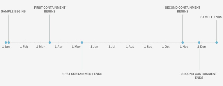
Fig. 1 gives an overview of the year 2020, showing the dates of our sample of 51 complete weeks (which are matched with the corresponding weeks from 2019) together with the bounds of the two containment periods which we examine. These containment period bounds pertain to the periods of peak restrictions (17 March through 10 May, and 30 October through 27 November), and correspond with the definitions used in the regression analysis below. Later sections examine the effects observable during these periods.
Fig. 1.
Timeline of sample and core containment dates, 2020.
3. The Cartes Bancaires CB data
Official data on consumer expenditure are typically available at the monthly frequency. As a result, short-run consumption fluctuations are poorly documented in the economic literature, particularly at the intra-day frequency. These relatively high-frequency fluctuations are nonetheless important in order to monitor economic activity on a day-to-day basis, particularly in the context of extreme events such as the pandemic. The filtering of predictable fluctuations within the week is also necessary in order to obtain a signal of the strength of economic activity updated daily in real time.
Here we use one of the richest data sets that has been adapted to real time analysis of economic activity: card payments. France has a mature bank card (carte bancaire) market, and Cartes Bancaires CB is one of the leading schemes, created by the French banks in 1984, and which by 2020 had more than 100 members (including payment service providers, banks and e-money institutions).7 As of 2019 there were 72 million CB cards in use in the CB system, and 1.8 million CB-affiliated merchants. Thanks to a partnership with Cartes Bancaires CB, we are able to observe each of the card transactions very precisely. A transaction is characterized by its value, the date of the transaction, the time of day recorded to the second, the geographical location of the merchant, the statistical classification of the type of purchase, and the type of purchasing channel used during the transaction, i.e. off-line or online. The detailed information on timing and location of the transaction, the nature of the merchant, and the type of purchase, online or off-line (point-of-sale), allows us to provide detailed descriptions of both intra-day and intra-week consumption fluctuations, and to contrast consumption patterns along the geographical and technological dimensions.
These data have an exceptional degree of coverage of transactions, allowing us to observe a significant proportion of all consumer expenditure in France. Consider a few comparisons of the Cartes Bancaires CB data set with national statistics provided for the full year 2019 by the National Institute of Statistics and Economic Studies (INSEE); GDP in France in 2019 was estimated as € 2,427 billion, with € 1,254 billion (52 percent of GDP) representing household consumption expenditure. Excluding fixed charges (rents, financial services, insurances) from household consumption expenditure, as these are typically paid by direct debits and credit transfers, the remaining part of consumer expenditure amounts to € 828 billion (34 percent of GDP). Comparing these figures with our sample of CB card payments in 2019 (€ 396 billion), the value of CB card payments represents 16 percent of the French GDP, 32 percent of the total household consumption expenditure, and finally 48 percent of total household consumption expenditure excluding fixed charges.8
The particular data set that we use in this paper represents a sample of approximately 20 billion transactions taken from the years 2019 and 2020; the sample spans periods before, during and after the two containments and comprises sub-samples of from 0.8 to 4.4 billion CB card transactions in 2019 and 2020 respectively, for total values of about € 34.9 to € 187.6 billion.9 A summary of descriptive statistics is provided in Table 1. We distinguish in particular five periods: the pre-containment period, i.e. January 6 to March 16; the first containment period from March 17 to May 10; the third period, after first containment, i.e. from May 11 to October 29; the second containment from 30 October to 27 November, and finally the period after the second containment, from November 29 to December 27. In each case the dates are defined by events in 2020, and the corresponding dates in 2019 are used for comparison.
Table 1.
Summary of descriptive statistics.
| Mean | Median | Obs. (billions) | Total value (billions €) | # Cards (millions) | # Merchants (millions) | |
|---|---|---|---|---|---|---|
| Panel A (2019) | ||||||
| Pre-containment | 39 | 20 | 1.30 | 51.2 | 61.0 | 1.01 |
| 1st containment | 40 | 20 | 1.49 | 59.1 | 62.6 | 1.03 |
| After 1st containment | 40 | 20 | 4.43 | 175.3 | 80.2 | 1.10 |
| 2nd containment | 40 | 21 | 1.14 | 45.7 | 61.2 | 1.02 |
| After 2nd containment | 41 | 22 | 0.84 | 34.9 | 58.2 | 1.00 |
| Mean | Median | Obs. (billions) | Total value (billions €) | # Cards (millions) | # Merchants (millions) | |
| Panel B (2020) | ||||||
| Pre-containment | 39 | 20 | 1.37 | 53.4 | 63.0 | 1.02 |
| 1st containment | 46 | 25 | 0.81 | 37.4 | 58.7 | 0.66 |
| After 1st containment | 41 | 20 | 4.60 | 187.6 | 82.3 | 1.09 |
| 2nd containment | 41 | 20 | 1.01 | 41.4 | 62.8 | 1.00 |
| After 2nd containment | 44 | 23 | 0.83 | 36.5 | 60.2 | 0.94 |
Notes: This table reports descriptive statistics on transactions, cards and merchants for the five periods of interest that occurred in 2020 (Panel B), with the analogous periods in 2019 (Panel A): pre-containment (6 January to 16 March); first containment (17 March to 10 May); after first containment (11 May to 29 October); second containment (30 October to 27 November); after second containment (29 November to 27 December). Mean and median pertain to the values of individual purchases, in euros.
We will compare the evolution of consumption expenditures for each period in the next sections. It is nonetheless clear even from the summary statistics in Table 1 that while the distributions of values are similar prior to the containment dates, there are large differences in the values of payments during the containment dates in 2019 and 2020: the average transaction value of a card payment increases (from 40 to 46 € ) as does the median (from 20 to 25 € ), while the total value declines precipitously during the first confinement.
An important feature of these data, which will be used in results below, is that the merchant address is relatively well determined. There are a number of common difficulties in inferring merchant address in transaction data; a merchant address may be a billing address or head office address, for example, with goods delivered from warehouses located elsewhere. However, the nature of the information recorded for French retail businesses mitigates some of these standard concerns.
A merchant’s payment terminal is configured with information relating to the merchant’s bank (bank code and server), the payment terminal (terminal number), and finally the identity of the merchant. The merchant information includes the business identification number (SIRET code), name and address. The SIRET code is assigned by the French National Institute of Statistics (INSEE), and allows identification of each physical establishment of a company (if these exist) and its location, via a unique SIRET code. That is, multiple physical locations of a company will be identified differently.
Here, we use this code to infer the postal code and business sector. However, rather than deriving the postal code from data fields associated with the card terminal used to process a payment, we use the INSEE open data platform which associates a current location of the establishment with each (location-specific) SIRET code.10 Using this platform, we can assign to each establishment a sector according to the French nomenclature of activities derived from the international ISIC nomenclature (International Standard Industrial Classification of Economic Activities).
The address or postal code of the merchant determined in this way lets us infer the location of a physical (off-line) transaction with reasonable accuracy. For online transactions, additional difficulties may arise, however. If the business is purely online and has no retail outlets, a transaction may be recorded at a billing address, but the good may be delivered from another location such as a warehouse. This may or may not be a concern, depending on the type of inference which one wishes to draw; for example, if we are characterizing transactions outside the home département, which of two external départements is deemed to be the location is irrelevant to the home/away-from home distinction. Some measurement error of this type can however arise in the exceptional case where the distinction between billing address and warehouse address will affect the home/away-from-home determination (e.g., billing address is in the home département, warehouse is not).
4. Changes in aggregate consumption during the containment
We begin by documenting the changed patterns of consumption expenditure observed during the periods of mobility restrictions and closures of non-essential activities.
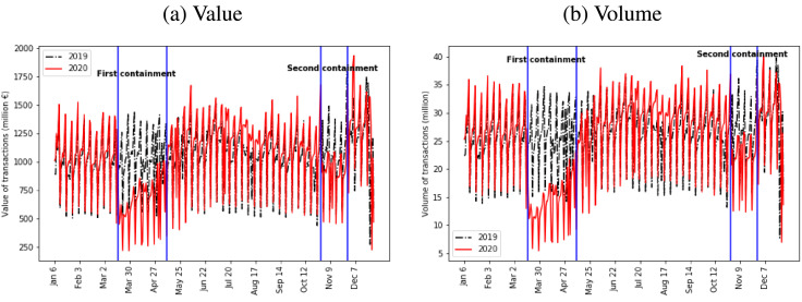
Fig. 2 displays the aggregate value and volume of transactions per day through calendar years 2019 and 2020. Several observations can be made: first, economic activity is very similar for the years 2019 and 2020 up to March 15, the date at which all places receiving non-essential public traffic are closed. Second, although this may be difficult to observe in the graphical representation, there was a sudden increase in activity of about 40 percent on March 16, one day before the beginning of the home containment. Third, with the containment in force from March 17, we observe a significant drop in activity of more than 60 percent in value and number of transactions in the weeks immediately following imposition of the containment, with the effect diminishing somewhat over the course of the containment period. Finally, although the consumer mobility restrictions were similar during the second containment on October 30 2020, we observe a less severe drop in aggregate transactions.
Fig. 2.
Daily fluctuations in aggregate transactions, January–December 2019–20.
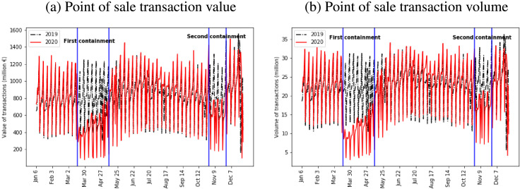
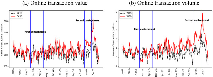
Fig. 3, Fig. 4 show the disaggregation of the total daily values and volume into point-of-sale and online transactions, again for the calendar years 2019 and 2020. Point-of-sale transactions, being the largest part of the total, show patterns similar to those of the total, as depicted in Fig. 2.
Fig. 3.
Daily aggregate POS transactions, 2019–2020.
Fig. 4.
Daily aggregate online transactions, 2019–2020.
Perhaps surprisingly, we note that at the beginning of the first containment there was also an immediate drop in online transactions, possibly attributable to the fact that many online purchases are of services such as travel and hospitality, which were greatly constrained for a time, as well as to the uncertainty of this period. Over the period of this first containment we see a rebound in online activity, which comes to exceed the previous year’s levels toward the end of the period. During the second containment, by contrast, online transactions were markedly higher than in the previous year throughout, suggestive of consumer learning and adaptation over the course of the first pandemic year.
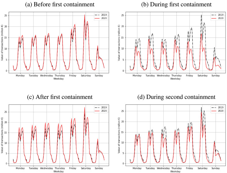
It is interesting to note that the difference between the first and second containments can also be observed in patterns of expenditure within the day and within the week. Fig. 5 displays the aggregate value of purchases by hour and day of the week, contrasting 2019 and 2020, for four periods of interest. Before the first containment, we observe a similar bi-modal distribution for each day from Monday to Saturday, and increasing economic activity in the course of the week. Consumption expenditure is highest on Saturday (+28% compared with the average of the other days of the week) and is lowest on Sunday (−46% compared with the average of the other days of the week); most stores are closed on Sunday because of legal restrictions. We also observe differences in intra-day variation within the week; Saturday and Sunday show higher peaks in the morning and in the afternoon, whereas activity is slightly higher in the afternoons for the remaining days of the week. Sunday afternoon differs markedly from the other days of the week, with an afternoon consumption peak much less marked than for the other days of the week.
Fig. 5.
Intra-Week Consumption Fluctuations, January–December 2019–20 (Value).
During the first containment, economic activity was more evenly distributed over the week, but maintained the significant drop in activity on Sunday. We also see that economic activity was more pronounced in the morning during containment, relative to the pre-containment period; each day of the week displayed a pattern of activity resembling a Sunday during the pre-containment period. Comparing panels (b) and (d), we observe a less marked change in the hourly and daily patterns of consumer expenditure during the second containment than was the case during the first. As was the case with the contrast between the online expenditure responses to the first and second containments, we see some suggestion of consumer learning or adaptation, which may have allowed consumers to remain closer to normal patterns during the second containment period.
The contrast between changes in online and POS expenditures during the containment periods, and evidence of consumers’ adaptation to the restrictions, are explored further and more formally in Section 6.
5. Changes in consumers’ mobility
As outlined in Section 2, the French government introduced policies designed to limit individuals’ mobility except for authorized reasons. In this section, we measure the corresponding changes in consumer mobility and expenditure outside the home city. First, we measure the distance in kilometres that each card travels between cities in the course of point-of-sale transactions, before, during and after the two mandatory containments. Second, we analyse home-city and external (‘away’) expenditure patterns, again comparing before-, during- and after-containment periods.
5.1. Consumer mobility across cities
To calculate consumer mobility, we apply the methodology developed in Bounie et al. (2020b). We measure the geographical distance between two distinct geographical purchasing locations such as cities, using the Haversine distance formula. The latter formula computes shortest distances between points on a sphere, as opposed to using road or rail network information. This measure requires precise information on merchants’ locations; fortunately, each transaction in our data contains a merchant identification number, a code which gives the precise postal address of the merchant including the postal code, which we use at the five-digit level.11
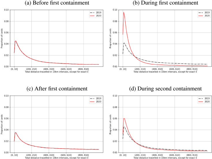
We use a sample of cards valid over the entire period 2019–2020; for comparability, we randomly select among cards valid throughout the years 2019 and 2020. Fig. 6 displays the distribution of distances travelled by 12.5 million cards, within Metropolitan France. The horizontal axes indicate the interval of distances travelled in 10 kilometre intervals, truncated at 1000 km and excluding zero km,12 while the vertical axis in each figure indicates the proportion of cards. In Fig. 6(a), we observe that before the first containment dates, the distances travelled by cards were virtually identical in 2019 and 2020. However, Fig. 6(b) shows quite a difference between 2019 and 2020; a much greater proportion of cards travelled only small distances during the first containment relative to the comparable period in 2019 (and in fact the average distance travelled was approximately one third). The effect is substantially different for the second containment; Fig. 6(c) again shows very similar patterns across the two years in the dates between the two containments, while Fig. 6(d) shows a smaller effect of the second containment on the distribution of distances travelled.
Fig. 6.
Distribution of distances travelled by cards between point-of-sale transactions.
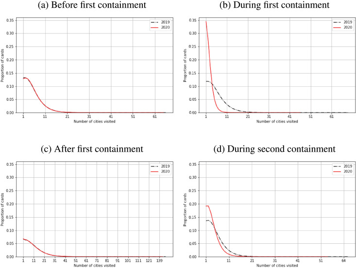
Fig. 7 describes a different indicator of mobility, the number of cities and towns in which each card is used. Again, we see no distinction between consumer mobility across cities in 2019 and 2020 in either of the non-containment periods (Figs. 7(a), 7(c)). However, we again observe both a substantial reduction in the measure of mobility during containment periods, and a marked difference between the two containments; we see in comparing Fig. 7, Fig. 7 that approximately 35% of cards were used in a single city during the first containment, compared with just under 20% during the second.
Fig. 7.
Distribution of number of cities visited per card.
These differences between effects of the two containments will be relevant to our later interpretation of differences in consumption effects across the two containment periods.
5.2. ‘Home’ and ‘away’ expenditures
In the previous sub-section we looked at consumer mobility without reference to a home base. Next we consider consumer expenditures in or outside the cardholder’s home location, to assess the impact of the containment periods. We start by defining a card’s home city or département as the location in which the largest number of transactions takes place13 ; next we compute the proportions of transaction values taking place in the home location, and externally (’away’) for each card, whether before or during the containment.14
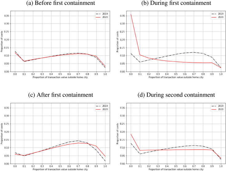
Fig. 8 plots the proportions of transactions made externally to the home city, at intervals of 0.1, during the relevant periods in 2019 and 2020. Before the first containment dates, we again observe almost identical distributions in 2019 and 2020 (Fig. 8(a)), with only a small proportion of cards, around 12%, making no transactions outside the home city, and with the largest proportion of cards making in the range of 70% of transactions externally. During the first containment, Fig. 8(b), we see a much larger proportion (over 35%) of cards being used only in the home city, with corresponding reductions in the proportions of cards making larger percentages of transactions outside. As well, again as observed with previous measures, the effect of the second containment is smaller.
Fig. 8.
Distribution of the value of consumer expenditures made within or outside the cardholders home city.
Further results describing consumers’ mobility across retailers are given in the Appendix. Collectively, these distributional shifts show that there were substantial changes in consumers’ movements during the containment periods, locally as well as among cities or regions, and that they were stronger during the first containment.
6. Modelling responses to the containment
We now turn to models with which to estimate the responses of the French economy to the shocks of the pandemic and containments. We begin by describing the methods and estimation strategy, and then present the main results.
6.1. Methodology
We use a standard difference-in-difference regression methodology to estimate the causal effect of the COVID-19 crisis. We compare the before- and after- containment changes in daily expenditure across the relevant periods in 2020 to those in the comparable periods of 2019; the treatment group corresponds with the year 2020, and the control group corresponds with the year 2019. We first contrast the pre-COVID period with the period following; the pre-treatment period is from January 6 through March 16 and the post-treatment period is from March 17 through December 27. Next we examine the two containment periods in a common model, using the containment period dates defined earlier, and treating the post-first- and post-second-containment periods separately. In each case, the high degree of stability in value and volume of daily card expenditure across the two years during the pre-containment dates (as documented below) suggests that the implicit counterfactual estimate, of 2020 expenditure in the absence of the crisis, is quite reliable.
Throughout this section we use models similar to those of Agarwal et al. (2007), Aaronson et al. (2012), Agarwal and Qian (2014) and Agarwal et al. (2019b), expressed here in first-differenced form, to study the average daily expenditure response to the containment during the COVID-19 crisis. We first use the following specification:
| (1) |
where the dependent variable is the change in the logarithm of either total value, total volume, or average value per card, of transactions carried out during the day of the year. is a binary variable equal to one for the days before the beginning of the first containment and is a binary variable that equals one for the days after its beginning (i.e., from March 17 2020). We also include dummy variables for special days such as public holidays and Valentine’s Day. The parameter in Eq. (1) captures an average 2020 daily expenditure response from mid-March through year end to the COVID-19 pandemic and containment policies, relative to the control period. This parameter is therefore an average over containment and non-containment periods. measures the difference in the spending trend between the years 2020 (treatment group) and 2019 (control group) during the pre-treatment days (compared with the benchmark period). The validity of inference from the difference-in-difference model requires that be statistically indistinguishable from zero.15
Next, we modify the first specification to distinguish the two main containment periods in the year 2020, adding indicators for the second containment and the periods before and after. Correspondingly, we use the specification:
| (2) |
with the four containment-related indicator variables corresponding with the periods March 17 through May 10 (1st containment), May 11 through October 29, October 30 through November 27 (2nd), and finally November 28 through December 27. The coefficients associated with and in Eq. (2) capture therefore the estimated average daily expenditure response during the containment periods.
Finally, in addition to the first two specifications, we want to study the dynamics of the daily spending response to the COVID-19 crisis. We therefore consider a model with daily or weekly dummies for particular days or weeks in 2020:
| (3) |
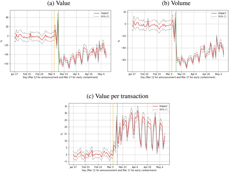
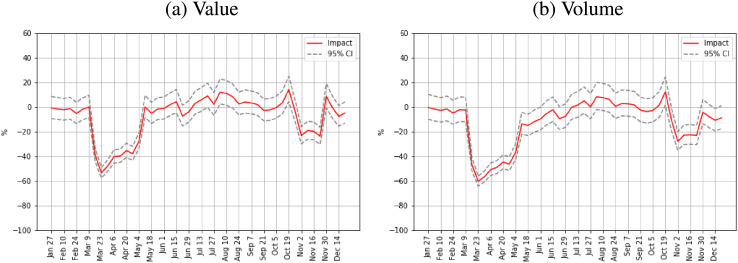
now represents either a daily or a weekly aggregate observation, measures the response on a particular day or week, and is the indicator variable for that day or week. The coefficient measures the immediate response in spending after the first speech of the French President. Similarly, coefficients capture the differences in spending between the years 2019 and 2020 in the pre-treatment days. The results can be interpreted as an event study and are represented here in Fig. 9, focusing on the first containment; analogous results at the weekly rather than daily level, for the full calendar year, are presented in Fig. 10. Values in the pre-treatment period should be approximately zero under the parallel trends assumption, as indeed we observe.
Fig. 9.
Estimated daily expenditure response dynamics.
Notes: This figure plots the coefficients estimated from Eq. (3), with = January 27 2020, January 28 2020, …, May 10 2020, along with their corresponding 95 percent confidence intervals. The -axis denotes the day and the -axis shows the estimated daily percentage response.
Fig. 10.
Estimated weekly expenditure response dynamics.
Notes: This figure plots the coefficients estimated from the weekly form of Eq. (3), with indicating weekly values for the weeks beginning January 27 2020 through December 21 2020, along with their corresponding 95 percent confidence intervals. The -axis denotes the date at weekly intervals and the -axis shows the weekly percentage spending response.
6.2. Mean response of card expenditure
Table 2 summarizes the estimation results for models (1), (2). Panel A gives results on average responses of card expenditures over the entire post-Covid part of the sample, from Eq. (1), while Panel B represents Eq. (2), estimating effects observed during the periods of interest described earlier. The dependent variables are the logarithm of total daily value of card spending in column (1), the logarithm of total daily volume of card spending in column (2), and the logarithm of value per card transaction in column (3). The coefficients associated with the indicator variables then measure the difference in daily expenditure measures in 2020 relative to the pre-treatment days in 2019.
Table 2.
Mean daily spending response to the COVID-19 containments.
| Panel A | log(total value) | log(total volume) | log(value per trans.) |
|---|---|---|---|
| (1) | (2) | (3) | |
| pre | 0.002 | −0.009 | 0.011 |
| (0.018) | (0.016) | (0.009) | |
| post | −0.098*** | −0.161*** | 0.064*** |
| (0.033) | (0.037) | (0.007) | |
| Constant | 0.059*** | 0.077*** | −0.018*** |
| (0.016) | (0.015) | (0.003) | |
| 0.375 | 0.322 | 0.244 | |
| Observations | 357 | 357 | 357 |
| # Transactions | 18.4 | 18.4 | 18.4 |
| Panel B | log(total value) | log(total volume) | log(value per trans.) |
| (1) | (2) | (3) | |
| pre | 0.002 | −0.009 | 0.011 |
| (0.018) | (0.016) | (0.009) | |
| containment 1 | −0.534*** | −0.690*** | 0.156*** |
| (0.053) | (0.05) | (0.01) | |
| after containment 1 | 0.037* | −0.003 | 0.04*** |
| (0.02) | (0.019) | (0.006) | |
| containment 2 | −0.211*** | −0.252*** | 0.041*** |
| (0.025) | (0.021) | (0.011) | |
| after containment 2 | −0.022 | −0.091*** | 0.069*** |
| (0.039) | (0.024) | (0.017) | |
| Constant | 0.059*** | 0.077*** | −0.018*** |
| (0.016) | (0.015) | (0.003) | |
| 0.791 | 0.851 | 0.584 | |
| Observations | 357 | 357 | 357 |
| #Transactions | 18.4 | 18.4 | 18.4 |
Notes: This table reports the average daily card spending response (Eqs. (1), (2)) to the COVID-19 crisis in the sample from January 6 through December 27. Panels A and B represent the estimation results of Eqs. (1), (2) respectively. The dependent variable is the logarithm of total daily value of card expenditure in column (1), the logarithm of total daily number of transactions in column (2) and the logarithm of value per card transaction in column (3). Indicator variables are defined on the periods given in the text. HAC standard errors are reported in parentheses. ***, **, * indicate significance at the 1%, 5% and 10% levels, respectively. The number of transactions is the size of the sample from which daily values of the dependent variables are computed.
In all three columns in both panels of Table 2, the coefficients estimated on the pre-treatment period variable (i.e., ) are both economically small and statistically insignificant, a result consistent with the hypothesis that the common trend assumption of the difference-in-difference setting is not violated.
Panel A estimates an average effect over the post-Covid period of the sample, which is divided into sub-periods in the results of Panel B; there we note large negative effects of the first containment on both value and volume, the latter greater in magnitude, corresponding with an increase in value per transaction. The second containment shows effects of the same directions and relative magnitudes, but less than half as large as the estimated effects of the first containment period. The after-containment periods show only small (and in several cases statistically insignificant) estimated differences relative to the corresponding periods in 2019. The smaller estimated effects of the second containment are compatible both with the hypothesis of consumer learning and adaptation, and with the observation that the restrictions of the second containment were somewhat milder. We return to these points below.
6.3. Dynamic response of card expenditure
We now turn to the daily dynamic evolution of the card expenditure response, before and during the first containment policy period. Figs. 9(a) to 9(c) plot the coefficients from Eq. (3) representing the estimated daily spending response dynamics, for January 27 2020 through May 10 2020, along with their corresponding 95 percent confidence intervals. In this and later plots of the evolution of coefficients, these coefficients are transformed to to represent percentage changes.16 The -axis denotes the day, and the -axis the percentage estimated expenditure response for the given day. Recall that March 13 2020 was the first day following the initial announcement, and March 17 2020 was the first day of containment.
The last day before the containment period, that is March 16, shows clear spikes in transaction values, volumes, and values per transaction; total transaction value increased by close to 40%, followed by a dramatic drop in the first days of containment, approximately stabilizing thereafter: as containment officially began on March 17 2020 at noon, there was a decrease in card transaction value of about 30%, followed by a further decrease of about 60% on March 18.17 The results are similar for total card transaction volumes, while average value per transaction significantly increased in the days after the first announcement window.
Fig. 10 plots the coefficients in weekly aggregates of the data, this time for the full sample period, including the second containment.18 We now see a more regular pattern of decline in both value and volume of transactions during the containment periods. Weekly value per transaction (not shown) increased during the first containment in particular, settling back to previous levels thereafter.
Overall, the results in Fig. 9, Fig. 10 suggest that consumers responded strongly to the containment restrictions and announcements, first with some anticipatory purchases in advance of the restrictions, followed by steep declines in the number of transactions, and an increase in the average size of each transaction as consumers economized on trips to physical stores. We turn next to two potential channels through which consumers could adapt to the shock induced by the pandemic and associated policy restrictions: substitution toward online purchases, and intertemporal substitution (delay).
6.3.1. POS vs. online dynamic response
The aggregate expenditure results described in the previous section may obscure important differences between traditional point-of-sale expenditures and online expenditures, which may have interesting implications. In this section we examine this off-line/online contrast, via a decomposition of the analysis of the previous section into off-line and online components.
Table 3 provides the regression results and numerical values corresponding with Panel B of Table 2, now decomposed into point-of-sale (offline) and online transactions.
Table 3.
Average daily POS and online expenditure response to the COVID-19 crisis.
| Off-line |
Online |
|||||
|---|---|---|---|---|---|---|
| log(total val.) | log(total vol.) | log(avg. val.) | log(total val.) | log(total vol. | log(avg. val.) | |
| (1) | (2) | (3) | (4) | (5) | (6) | |
| pre | 0.019 | −0.002 | 0.021 | −0.051*** | −0.039** | −0.012 |
| (0.027) | (0.021) | (0.013) | (0.019) | (0.015) | (0.011) | |
| cont. 1 | −0.72*** | −0.83*** | 0.109*** | −0.116** | −0.131*** | 0.015 |
| (0.065) | (0.059) | (0.017) | (0.05) | (0.035) | (0.018) | |
| after cont. 1 | 0.029 | −0.021 | 0.05*** | 0.068*** | 0.112*** | −0.044*** |
| (0.026) | (0.024) | (0.007) | (0.013) | (0.015) | (0.01) | |
| cont. 2 | −0.371*** | −0.370*** | −0.001 | 0.145*** | 0.213*** | −0.068*** |
| (0.035) | (0.029) | (0.011) | (0.05) | (0.035) | (0.019) | |
| after cont. 2 | −0.082** | −0.153*** | 0.072*** | 0.169*** | 0.216*** | −0.047** |
| (0.039) | (0.027) | (0.015) | (0.048) | (0.034) | (0.02) | |
| Constant | 0.042* | 0.073*** | −0.031*** | 0.107*** | 0.091*** | 0.016** |
| (0.024) | (0.02) | (0.004) | (0.006) | (0.009) | (0.007) | |
| 0.799 | 0.855 | 0.432 | 0.441 | 0.597 | 0.297 | |
| Obs. | 357 | 357 | 357 | 357 | 357 | 357 |
| # Trans. | 15.6 | 15.6 | 15.6 | 2.7 | 2.7 | 2.7 |
Notes: This table reports the average daily card transaction response (Eq. (2)) to the COVID-19 crisis in the sample from January 6 through December 27, analogous to Panel B of Table 2, but with point-of-sale and online transactions modelled separately. The dependent variable is the logarithm of total daily value of card expenditure in columns (1) and (4), the logarithm of total daily number of transactions in columns (2) and (5) and the logarithm of average value per card transaction in columns (3) and (6), in each case treating point-of-sale and online separately. Indicator variables are defined on the periods given in the text. HAC standard errors are reported in parentheses. ***, **, * indicate significance at the 1%, 5% and 10% levels, respectively. The number of transactions is the size of the sample from which daily values of the dependent variables are computed.
Consider first containment 1. Online transactions also show a decline in total value and total volume, although of much smaller magnitude than for point-of-sale transactions. Online, there was no significant change in average value per transaction during the containment. It may at first seem surprising that the value of online commerce declined, initially, at all. However, online commerce comprises numerous different categories, some of which, such as travel expenditures, were also curtailed by the containment; others such as informational content can be purchased and consumed online (e.g. digital books, music, newspapers) and so might be unaffected or even increased. As well, the general increase in economic uncertainty associated with the beginning of the pandemic and containment may have led consumers to reduce discretionary purchases.
By contrast, in the period after the first containment, and particularly during the second containment and thereafter, we observe substantial and significant increases in both value and volume of online purchases, while POS purchases again declined strongly during the second containment, although less strongly than during the first. The results for online purchases suggest consumer learning, and that the effect of this learning was maintained through the sample period, allowing consumers to mitigate the effects of the second containment immediately. Although the milder overall effect of the second containment, observed in Table 2, may in part be the result of somewhat less stringent restrictions or lower anxiety in the population, the results of the decomposition into online and POS transactions suggests that consumer learning and adaptation, through more widespread familiarity with the process of online purchasing, may also have contributed to mitigating the effects on overall consumption.
In the next section, we examine adaptation via a different decomposition of transactions: by type of purchase.
7. Sectoral heterogeneity and inter-temporal substitution
Another form of adaptation available to consumers, for some expenditures, is intertemporal: purchases may be delayed. The degree to which this is possible differs among types of purchase; the exceptional level of detail available in the present data allows us to decompose purchases into classes and thereby also to document the large sectoral heterogeneity in the severity of the two Covid shocks. In this section we describe how the consumption of durable, non-durable, and hospitality goods evolved during the first two containments, and draw attention to implications for adaptation to the shocks.
We start by focusing on expenditures on durables. We define durable goods as cars, motorcycles, home appliances, IT, furniture, and jewelry.19 The dynamics of expenditure on durables is crucial in understanding the underlying mechanisms driving consumption dynamics, and in particular intertemporal substitution. During times of economic uncertainty, we expect that consumers will postpone purchasing durable goods such as those described above; durables provide utility over multiple periods, so that one can postpone purchases in times of economic hardship, while still benefiting from the level of durables accumulated.
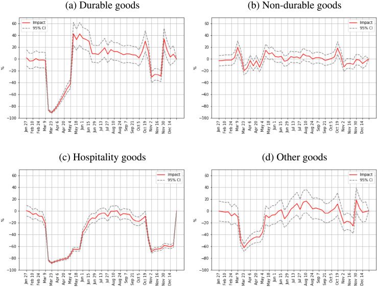
Fig. 11(a) reports the evolution of consumption expenditures on durables and confirms this expectation. After a very large decline during the first confinement period, expenditures on durable goods bounced back significantly right afterward, and indeed this strong pattern of intertemporal reallocation of expenditures enabled the economy to recoup a significant share of the losses made during the first lockdown period. The same pattern prevailed for the second containment, although the fall observed during this period was less than half that of the first containment.
Fig. 11.
Estimated weekly expenditure dynamics, by sector.
Notes: This figure plots the coefficients estimated from Eq. (3), using a sectoral disaggregation of the total value of transactions, with indicating weekly values for the weeks beginning January 27 2020 through December 21 2020, along with their corresponding 95 percent confidence intervals. The -axis denotes the date at weekly intervals and the -axis shows the weekly percentage spending response.
This pattern contrasts with that of non-durable goods, reported in Fig. 11(b), for which consumers cannot readily postpone expenditures. Non-durable goods are products that are purchased for consumption over a short time horizon, and include in the present study purchases in supermarkets and grocery stores, florists, drugstores, beauty stores, etc.20 While we do observe some increase in non-durables transactions after the lockdowns, consistent with some delayed gratification, the effect is notably smaller than for durables.
Finally in Fig. 11(c), we report the evolution of expenditures in the hospitality sector, defined as restaurants and cafés, culture and entertainment, libraries, and sports activities.21 The patterns are notably different compared with those of durable goods. Although the hospitality sector was also severely affected by the lockdowns, it did not experience a rebound thereafter to above pre-COVID levels. Various administrative restrictions remained in place in these sectors throughout the summer months; furthermore, hospitality expenditures went into decline from the end of August, as new cases started to rise in France, prompting new administrative measures restricting consumption in these sectors.
We draw two conclusions from this examination of sectoral heterogeneity of transactions. First, there is evidence that intertemporal substitution provided another channel (in addition to substitution toward online purchases) by which consumers were able to adapt to the shocks and mitigate their effects; the recouping of ‘lost’ transactions during the containments is most clearly visible for durable goods, for which the effect would be expected to be strongest. Second, the strong increase in durables purchases following the first containment suggests that the overall impact on the economy through lost consumption was substantially reduced by the possibility of delaying, rather than eliminating, purchases.
8. Inter-regional trade effects
Changes in consumer mobility imply changes in consumers’ purchases from other regions, and we expect differential economic effects across regions from the reduction in external visitors. We now investigate these changes, and in particular the impact of the pandemic and containment on inter-regional retail trade.
8.1. Inter-regional linkage measure
We begin by defining inter-regional linkage measures based on a consumer’s home département, which we define here as the location in which the largest number of transactions takes place during a pre-pandemic reference period, January 2019 through February 2020. We will consider measures based on either number of inter-regional purchasers, number of retailers visited outside the home region, or total value or volume of these transactions: first, the number of cards with home in département which made at least one transaction in département during a given month, second, the number of retailers visited during these external transactions, and finally the total value of transactions recorded in département during a given month, by cards with home in département . Note that the first of these measures the number of -cardholders who made at least one purchase in , not the total number of their purchases.
For a given time period, let index all cards with ‘home’ in département , let be the indicator function that takes the value 1 if card made at least one purchase in département during the period, let be the number of merchants from which purchases were made (either at point of sale or online), and let be the total value or volume of transactions on card made at a merchant located in département . Then the inter-regional consumer mobility measures are , , and . We will use the generic symbol for any of these.
8.2. Econometric models
We will evaluate the impact of the containment on each of these inter-regional measures, through the main containment periods, and also over one-month periods. As above, we use a difference-in-difference approach. In order to approximate percentage changes in the regression models, we take the logarithm of as dependent variable, where this represents any of the measures of inter-regional consumer activity between départements and during time period . The model may be represented as:
| (4) |
where captures individual fixed effects in order to absorb time-invariant factors in the pairing is a vector of time-related dummy variables to control for a time-varying trend in the inter-regional trade measures. The dummy variable is defined as 1 for 2020 sample observations, and 0 otherwise; is defined as 1 for dates following the beginning of the containment period; then captures the average response of the dependent variable during the containment period. As in Section 6, we then extend this model to treat the two containment periods, and the periods following them, separately. To investigate the dynamic evolution of the impact, we also estimate the model in a form which separates the effects of each month during the period of interest:
| (5) |
where the set , is a binary indicator variable for each month , and estimates the impact of the set of conditions (containment or other) prevailing during the corresponding month.
8.3. Estimates: Average inter-regional response
We begin by estimating the average effect on monthly inter-regional consumer activity measures, and report the results in Table 4.22 This table uses all four different versions of the dependent variable: total value, number of transactions, number of cards making at least one purchase, and number of retailers visited. In each case we use the logarithm of the corresponding definition of , as described above, for a pairing of two départements and a particular time period.
Table 4.
Models of inter-regional consumer transactions.
| Panel A | Value | Volume | # Cards | # Retailers |
|---|---|---|---|---|
| (1) | (2) | (3) | (4) | |
| Treat × Post | −0.700*** | −0.647*** | −0.788*** | −0.624*** |
| (0.004) | (0.004) | (0.004) | (0.003) | |
| Constant | 9.328*** | 5.724*** | 4.946*** | 4.901*** |
| (0.006) | (0.006) | (0.005) | (0.005) | |
| Fixed effects: département pair, month | yes | yes | yes | yes |
| 0.473 | 0.505 | 0.576 | 0.524 | |
| Observations | 216,244 | 216,244 | 216,244 | 216,244 |
| Panel B | Value | Volume | # Cards | # Retailers |
| (1) | (2) | (3) | (4) | |
| Treat × Post × Containment 1 | −1.318*** | −1.276*** | −1.484*** | −1.263*** |
| (0.006) | (0.005) | (0.005) | (0.005) | |
| Treat × Post × AfterContainment 1 | −0.266*** | −0.217*** | −0.300*** | −0.178*** |
| (0.004) | (0.004) | (0.003) | (0.003) | |
| Treat × Post × Containment 2 | −1.118*** | −0.973*** | −1.258*** | −1.010*** |
| (0.007) | (0.006) | (0.006) | (0.005) | |
| Treat × Post × AfterContainment 2 | −0.611*** | −0.593*** | −0.682*** | −0.556*** |
| (0.006) | (0.006) | (0.005) | (0.004) | |
| Constant | 9.328*** | 5.724*** | 4.946*** | 4.901*** |
| (0.006) | (0.005) | (0.005) | (0.005) | |
| Fixed effects: département pair, month | yes | yes | yes | yes |
| 0.559 | 0.598 | 0.684 | 0.641 | |
| Observations | 216,244 | 216,244 | 216,244 | 216,244 |
Notes: This table reports estimates of models of inter-regional consumer expenditure response to the pandemic conditions. The dependent variable is the logarithm of each choice of is a dummy variable for the relevant period of the year 2020 and is a binary indicator variable that equals 1 for the particular sub-period of interest. All regressions include time and département-pair fixed effects. Robust standard errors clustered at département-pair level are reported in parentheses. ***, **, * indicate significance at the 1%, 5% and 10% levels, respectively.
Panel A shows effects over the full post-Covid period of 2020, that is from mid-March through the end of our sample. We see that all measures show strong and highly significant effects on inter-regional retail transactions. Recall that we use the transformation to estimate the percentage change; is approximately −0.5 or a 50% reduction, and this set of measures shows declines ranging from approximately 46% to 54% over this full period.
Panel B of Table 4 reports estimation results for sub-periods defined earlier. We see quite dramatic declines during the both containment periods, although once again the effects observed during the second containment are somewhat smaller. Applying the transformation in order to interpret the results, we see first- and second- containment period effects of −73% and −67% respectively. It is interesting to note that inter-regional transaction measures did not recover as rapidly in post-containment periods as did overall economic activity, as estimated in Section 6; inter-regional transactions remained persistently below previous levels during the post-containment periods.
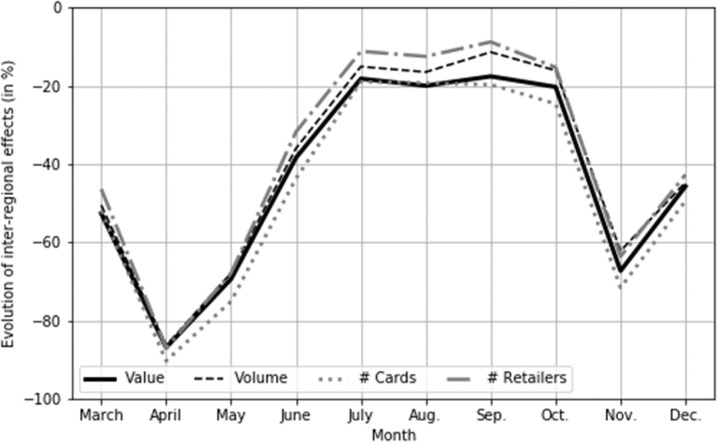
Fig. 12 provides a graphical overview of the evolution of these effects during the post-Covid part of our sample, derived from regressions analogous to those of Panel B of Table 4, but where each month in the period March through December 2020 is treated separately. The value plotted is , where is the regression coefficient for month within this period. Within the first containment, April was the month of maximum effect.
Fig. 12.
Evolution of inter-regional effects.
9. Conclusion
It is inevitable that conditions such as those of the COVID-19 pandemic must have profound effects on economic life, and in particular on individuals’ movements and consumption of goods and services. However, our ability to learn about and measure these effects using economic data from the standard official sources is limited by the frequency and geographical resolution of these data.23
Nonetheless, the individual transaction data available through Cartes Bancaires CB offer the opportunity to study the effects of the pandemic, and the policies introduced to limit it, at an exceptional level of detail. These data are not only available at an extremely fine time scale, but also contain locational information allowing us to study local effects and individual movements. This information, recorded for billions of transactions, allows us to make a number of measurements and draw a number of conclusions that would be obscured in aggregate official consumption data.
First, by measuring effects at daily and weekly scales and over periods corresponding with the core periods of restriction on individual movement, we estimate the degree to which economic activity was curtailed along a number of dimensions: particularly the value and volume of transactions, but also distances travelled and numbers of cities or retailers visited per card. We measure the evolution of the reduction of consumer transactions over time and observe that the effects were most pronounced at the beginning of the first containment period and were of smaller magnitude, but nonetheless very substantial, during the second. The pandemic shock and restrictions on individual movement also reduced consumers’ purchases outside their home regions, and therefore inter-regional retail trade, and had differential impacts on different regions of France. We observe large reductions in measures of inter-regional transactions, consistent with the containment restrictions having been well respected throughout the territory of metropolitan France.
Two other features of these data, the ability to distinguish online from point-of-sale purchases and the ability to identify the economic sector of a purchase, allow us to draw conclusions with respect to consumers’ ability to adapt to the shocks and mitigate their effects, either through substitution toward online purchases, or inter-temporal substitution, in sectors where one or both of these was feasible. With respect to online transactions, we observe that while these were initially depressed at the beginning of the first containment (although to a lesser degree than point-of-sale), online transactions recovered during this period and rose quickly during the second containment period, reducing the overall impact of these periods on consumer expenditure. The difference between these two periods suggests that knowledge of online shopping mechanisms increased in the population, and the post-containment results suggest some persistent effects resulting from this learning. As well, the decomposition of transactions into durable and non-durable goods, hospitality and other purchases allows us to observe that durables purchases jumped to above-normal levels immediately after the containments, an observation which does not appear to a comparable degree for other classes of purchase. This observation is consistent with intertemporal substitution by consumers, a further channel by which they may be able to adapt and mitigate the effects of shocks.
The scale of the pandemic and of the restrictions imposed in response were unprecedented in the post-war era, as were the magnitudes of the economic effects. The possibility of using transaction data to measure and track the sizes of these impacts, on consumption, mobility and regional economic activity, is potentially of great value to policy makers in guiding decisions. Equally important, the high-frequency measurements available allow us to observe more subtle features of consumer behaviour than the changes in activity alone, in particular adaptation to mitigate the effects of shocks, both on the individual and on the economy.
Footnotes
This research has been made possible by the collaboration of Groupement des Cartes Bancaires CB, and was conducted within the Research Chair “Digital Finance” under the aegis of the Risk Foundation, a joint initiative by Groupement des Cartes Bancaires CB, Télécom Paris and University of Paris 2 Panthéon-Assas. We would like to thank Hafid Chakir, Philippe Durand, Ludovic Francesconi, Kim Hyunh, Niels Johannesen, Katérina Levallois, Saeideh Monirijavid, Loys Moulin, Francisco Rivadeneyra, Samuel Willy, the editors and two anonymous referees for their helpful comments on earlier versions of the paper.
These data were made available thanks to a partnership with Cartes Bancaires CB, and we exploit the card payments data in accordance with the EU General Data Protection Regulation, in application of Article 89. We use the abbreviation ‘CB’ to indicate the source of the card payments.
Other types of data source have also been explored; Hassan et al. (2020) have developed text-based measures of the costs, benefits, and risks listed firms in the US and over 80 other countries associate with the spread of COVID-19. They identify which firms expect to gain or lose from an epidemic disease and which are most affected by the associated uncertainty as a disease spreads in a region or around the world. They find that firms’ primary concerns relate to the collapse of demand, increased uncertainty, and disruption in supply chains. Bartik et al. (2020) use survey data to shed light on how COVID-19 is affecting small businesses. They confirm mass layoffs, closures, and financial fragility for small businesses.
Bounie et al. (2020a) evaluate the dynamics of cash withdrawals during the first containment using data from a major French bank, and show that they are 15% below their pre-crisis levels. This suggests that consumers have also significantly moved away from cash payments in response to the pandemic.
The Coronavirus Resource Center, https://coronavirus.jhu.edu, provides further information and numerical detail.
A travel certificate was required to leave one’s home, and travel between regions was prohibited.
A third confinement period, beginning 3 April 2021 for a duration of four weeks, is beyond the span of our available data sample.
We use the abbreviation ‘CB’ to indicate the source of the card payments. CB cards can be immediate-debit cards, but also deferred-debit cards (‘charge cards’ that require the balance to be paid in full each month), or credit cards (cards with a credit line). A peculiarity of the French card market is that merchants who accept CB cards will make no distinction between debit cards and the other types.
CB card payments do not capture all consumer spending in France. Some expenses are indeed paid in cash (mainly for low-value transactions) or with other payment instruments such as transfers and direct debits (used to pay recurring bills such as electricity), or with cheques (used to pay large- value transactions).
We limit the sample to Metropolitan France, which excludes the overseas territories.
See the open data platform at the following address (https://www.sirene.fr/sirene/public/static/open-data).
For a more formal definition of the measure, see Bounie et al. (2020b). It is important to note that we exclude online transactions to calculate consumer mobility.
Approximately 38% of cards travelled zero km during the first containment, while the comparable figure is 11% for the same period of the previous year.
We use the before-containment period to define the cardholder’s home region.
For more details concerning these measures, see Bounie et al. (2020b).
Note that the difference-in-difference estimator assumes that in the absence of the treatment, average daily spending in the two years would have changed in the same way throughout the observed periods. Consequently, any difference observed after the containment announcement period is attributed to the COVID-19 crisis.
Because our dependent variables are specified in logarithmic form, the coefficients on indicator variables can be interpreted as the change in when a given condition holds. For a proportionate change in , is and although this is approximately equal to for near zero, the standard transformation directly provides the proportionate change.
Sunday, March 15 2020 was a day of warm and sunny weather in much of France, and official directives to minimize non-essential contacts were not universally respected. President Macron spoke again on the evening of March 16 2020 on the seriousness of the situation and the necessity of an official containment.
Note that -axis values are for the week following the indicated date: for instance, the -axis value January 27 2020 corresponds with the week of January 27, 2020 to February 2, 2020, and February 3 2020 with the week of February 3 2020 to February 9 2020, and so on.
This corresponds with the following sectors in the French NAF classification of sectors: “451”, “453”,“454”, “474”, “475”.
We use the following codes in the French NAF classification: “4711”, “4781”, “4776”, “4773”, “9602”, “9604”.
The sector codes are respectively “56”, “90”, “91” and “93” in the French NAF classification.
Most results in the following tables are statistically significant at the 1% level, and we will not generally refer to statistical significance unless absent.
For example, Galbraith and Tkacz (2013) studied the response of consumer expenditure in Canada to a number of events including the SARS epidemic and the major electrical blackout, both in 2003; although some daily debit card data were available for that study, it was limited by the fact that these data were nationally aggregated, whereas the effect of shocks was localized.
Appendix. Consumer mobility across retailers
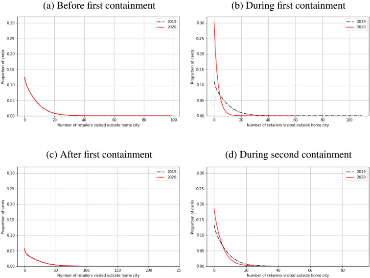
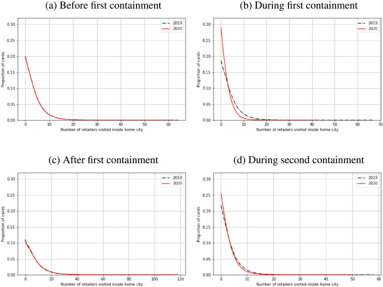
The distinction between home and away expenditure patterns is also visible in the number of point-of-sale retailers visited before and during containment. Recall that in addition to containment, French government policy imposed the closure of non-essential public places of business such as hotels, restaurants, and bars. Fig. 13, Fig. 13 exhibit the number of retailers from which any purchases were made before and during the first containment. We see that the number of retailers making sales was substantially lower during the first containment in 2020 than at the same period in 2019. More precisely, 30% of cards were used in retailers located in the home city during the first containment, and in contrast, about 11% of cards were used only in the home city at the same period in 2019. (see Fig. 14).
Fig. 13.
Number of retailers visited outside home city.
Fig. 14.
Number of retailers visited inside home city.
The effect is again smaller, but remains clearly discernible, in the period of the second containment.
References
- Aaronson Daniel, Sumit Agarwal, Eric French. The spending and debt response to minimum wage hikes. Amer. Econ. Rev. 2012;102(7):3111–3139. doi: 10.1257/aer.102.7.3111. URL http://www.aeaweb.org/articles?id=10.1257/aer.102.7.3111. [DOI] [Google Scholar]
- Agarwal S., Jensen J.B., Monte Ferdinando. National Bureau of Economic Research; 2019. The Geography of Consumption: Working Paper 23616. [Google Scholar]
- Agarwal Sumit, Liu Chunlin, Souleles Nicholas S. The reaction of consumer spending and debt to tax rebates—Evidence from consumer credit data. J. Polit. Econ. 2007;115(6):986–1019. URL http://www.jstor.org/stable/10.1086/528721. [Google Scholar]
- Agarwal Sumit, Qian Wenlan. Consumption and debt response to unanticipated income shocks: Evidence from a natural experiment in Singapore. Amer. Econ. Rev. 2014;104(12):4205–4230. doi: 10.1257/aer.104.12.4205. [DOI] [Google Scholar]
- Agarwal Sumit, Qian Wenlan, Yeung Bernard Y., Zou Xin. Mobile wallet and entrepreneurial growth. AEA Pap. Proc. 2019;109:48–53. doi: 10.1257/pandp.20191010. [DOI] [Google Scholar]
- Alfaro Laura, Chari Anusha, Greenland Andrew N., Schott Peter K. Aggregate and Firm-Level Stock Returns During Pandemics, in Real Time. National Bureau of Economic Research; 2020. (Working Paper Series). URL http://www.nber.org/papers/w26950. [DOI] [Google Scholar]
- Alon Titan M, Doepke Matthias, Olmstead-Rumsey Jane, Tertilt Michèle. The Impact of COVID-19 on Gender Equality. National Bureau of Economic Research; 2020. (Working Paper Series). URL http://www.nber.org/papers/w26947. [DOI] [Google Scholar]
- Andersen, A.L, Hansen, E.T, Johannesen, N., Sheridan, A., 2020. Consumer Reponses to the COVID-19 Crisis: Evidence from Bank Account Transaction Data. Working Paper, URL. [DOI] [PMC free article] [PubMed]
- Atkeson Andrew. What Will Be the Economic Impact of COVID-19 in the US? Rough Estimates of Disease Scenarios. National Bureau of Economic Research; 2020. (Working Paper Series). URL http://www.nber.org/papers/w26867. [DOI] [Google Scholar]
- Atkeson Andrew. How Deadly Is COVID-19? understanding the Difficulties with Estimation of Its Fatality Rate. National Bureau of Economic Research; 2020. (Working Paper Series). URL http://www.nber.org/papers/w26965. [DOI] [Google Scholar]
- Baker Scott R. Debt and the response to household income shocks: Validation and application of linked financial account data. J. Polit. Econ. 2018;126(4):1504–1557. doi: 10.1086/698106. [DOI] [Google Scholar]
- Baker Scott R., Bloom Nicholas, Davis Steven J., Kost Kyle J., Sammon Marco C., Viratyosin Tasaneeya. The Unprecedented Stock Market Impact of COVID-19. National Bureau of Economic Research; 2020. (Working Paper Series). URL http://www.nber.org/papers/w26945. [DOI] [Google Scholar]
- Baker Scott R., Farrokhnia Robert A., Meyer Steffen, Pagel Michaela, Yannelis Constantine. How does household spending respond to an epidemic? consumption during the 2020 COVID-19 pandemic. Rev. Asset Pricing Stud. 2020;10(4):834–862. doi: 10.1093/rapstu/raaa009. [DOI] [Google Scholar]
- Bartik Alexander W., Bertrand Marianne, Cullen Zoë B., Glaeser Edward L., Luca Michael, Stanton Christopher T. How are Small Businesses Adjusting to COVID-19? Early Evidence from a Survey. National Bureau of Economic Research; 2020. (Working Paper Series). URL http://www.nber.org/papers/w26989. [DOI] [Google Scholar]
- Bounie, David, Camara, Youssouf, Fize, Etienne, Galbraith, John, Landais, Camille, Lavest, Chloe, Pazem, Tatiana, Savatier, Baptiste, 2020a. Consumption Dynamics in the COVID Crisis: Real Time Insights from French Transaction & Bank Data. CEPR Discussion Papers, (15474), URL.
- Bounie David, Camara Youssouf, Galbraith John. Telecom Paris; 2020. Online Commerce, Intra-Regional Retail Trade, and the Evolution of Gravity Effects: Technical Report. [Google Scholar]
- Carvalho Vasco M, Hansen Stephen, Ortiz Álvaro, Garcí a Juan Ramón, Rodrigo Tomasa, Rodriguez Mora Sevi, Ruiz José. Tracking the COVID-19 crisis with high-resolution transaction data. R. Soc. Open Sci. 2021;8(8) doi: 10.1098/rsos.210218. [DOI] [PMC free article] [PubMed] [Google Scholar]
- Chen, Haiqiang, Qian, Wenlan, Wen, Qiang, 2020. The Impact of the COVID-19 Pandemic on Consumption: Learning from High Frequency Transaction Data. Working Paper, URL.
- Chiou Lesley, Tucker Catherine. Social Distancing, Internet Access and Inequality. National Bureau of Economic Research; 2020. (Working Paper Series). URL http://www.nber.org/papers/w26982. [DOI] [Google Scholar]
- Di Maggio Marco, Kermani Amir, Keys Benjamin J., Piskorski Tomasz, Ramcharan Rodney, Seru Amit, Yao Vincent. Interest rate pass-through: Mortgage rates, household consumption, and voluntary deleveraging. Amer. Econ. Rev. 2017;107(11):3550–3588. doi: 10.1257/aer.20141313. URL https://www.aeaweb.org/articles?id=10.1257/aer.20141313. [DOI] [Google Scholar]
- Dingel Jonathan I., Neiman Brent. How Many Jobs Can be Done at Home? National Bureau of Economic Research; 2020. (Working Paper Series). URL http://www.nber.org/papers/w26948. [DOI] [Google Scholar]
- Eichenbaum Martin S., Rebelo Sergio, Trabandt Mathias. The Macroeconomics of Epidemics. National Bureau of Economic Research; 2020. (Working Paper Series). URL http://www.nber.org/papers/w26882. [DOI] [Google Scholar]
- Galbraith John W., Tkacz Greg. Analyzing economic effects of September 11 and other extreme events using debit and payments system data. Anal. PolitiquesCan. Public Policy. 2013;39(1):119–134. [Google Scholar]
- Guerrieri Veronica, Lorenzoni Guido, Straub Ludwig, Werning Iván. Macroeconomic Implications of COVID-19: Can Negative Supply Shocks Cause Demand Shortages? National Bureau of Economic Research; 2020. (Working Paper Series). URL http://www.nber.org/papers/w26918. [DOI] [Google Scholar]
- Hassan Tarek Alexander, Hollander Stephan, van Lent Laurence, Tahoun Ahmed. Firm-Level Exposure to Epidemic Diseases: Covid-19, SARS, and H1N1. National Bureau of Economic Research; 2020. (Working Paper Series). URL http://www.nber.org/papers/w26971. [DOI] [Google Scholar]
- INSEE . 2020. Point de Conjoncture. URL https://www.insee.fr/en/statistiques/4479775?sommaire=4473307. [Google Scholar]
- Johnson David S., Parker Jonathan A., Souleles Nicholas S. Household expenditure and the income tax rebates of 2001. Amer. Econ. Rev. 2006;96(5):1589–1610. doi: 10.1257/aer.96.5.1589. URL https://www.aeaweb.org/articles?id=10.1257/aer.96.5.1589. [DOI] [Google Scholar]
- Jones Callum J., Philippon Thomas, Venkateswaran Venky. Optimal Mitigation Policies in a Pandemic: Social Distancing and Working from Home. National Bureau of Economic Research; 2020. (Working Paper Series). URL http://www.nber.org/papers/w26984. [DOI] [Google Scholar]
- Kaplan Greg, Violante Giovanni L. A model of the consumption response to fiscal stimulus payments. Econometrica. 2014;82(4):1199–1239. URL http://www.jstor.org/stable/24029251. [Google Scholar]
- Kuchler Theresa, Russel Dominic, Stroebel Johannes. The Geographic Spread of COVID-19 Correlates with Structure of Social Networks as Measured by Facebook. National Bureau of Economic Research; 2020. (Working Paper Series). [DOI] [PMC free article] [PubMed] [Google Scholar]
- McKibbin Warwick J., Roshen Fernando. The Global Macroeconomic Impacts of COVID-19: Seven Scenarios. CAMA Working Paper; 2020. (Working Paper Series). [Google Scholar]
- OCDE . 2020. Coronavirus: The World Economy at Risk. URL https://www.oecd.org/coronavirus/en/ [Google Scholar]
- Piguillem, Facundo, Shi, Liyan Shi, 2020. The Optimal COVID-19 Quarantine and Testing Policies. In: Working Paper Series.
- Souleles Nicholas S. The response of household consumption to income tax refunds. Amer. Econ. Rev. 1999;89(4):947–958. doi: 10.1257/aer.89.4.947. URL https://www.aeaweb.org/articles?id=10.1257/aer.89.4.947. [DOI] [Google Scholar]


