SuperMAP: Deep Ultrafast MR Relaxometry with Joint Spatiotemporal Undersampling

Abstract

Purpose:

To develop an ultrafast and robust MR parameter mapping network using deep learning.

Methods:

We design a deep learning framework called SuperMAP that directly converts a series of undersampled (both in k-space and parameter-space) parameter-weighted images into several quantitative maps, bypassing the conventional exponential fitting procedure. We also present a novel technique to simultaneously reconstruct T1rho and T2 relaxation maps within a single scan. Full data were acquired and retrospectively undersampled for training and testing using traditional and state-of-the-art techniques for comparison. Prospective data were also collected to evaluate the trained network. The performance of all methods is evaluated using the parameter qualification errors and other metrics in the segmented regions of interest.

Results:

SuperMAP achieved accurate T1rho and T2 mapping with high acceleration factors (R = 24 and R = 32). It exploited both spatial and temporal information and yielded low error (normalized mean square error of 2.7% at R = 24 and 2.8% at R = 32) and high resemblance (structural similarity of 97% at R = 24 and 96% at R = 32) to the gold standard. The network trained with retrospectively undersampled data also works well for the prospective data (with a slightly lower acceleration factor). SuperMAP is also superior to conventional methods.

Conclusion:

Our results demonstrate the feasibility of generating superfast MR parameter maps through very few undersampled parameter-weighted images. SuperMAP can simultaneously generate T1rho and T2 relaxation maps in a short scan time.

1. INTRODUCTION

Quantitative MRI relaxation times, like the time for spin-lattice relaxation (T1), the time for spin-spin relaxation (T2), and the time for spin-lattice relaxation at rotating frame (T1rho), are regarded as essential imaging biomarkers for diagnosis of a range of diseases.^1–6 To perform parameter mapping, conventional methods require repeated scans of the same anatomical structure with varying sequence parameters like multiple echo times (TEs) and flip angles (FAs), or various inversion recovery times (TIs), which limits its wide clinical use.^7,8 Accordingly, the new technique to accelerate parameter mapping is highly needed and remains an interest in MR research.

To speed up data acquisition, compressed sensing (CS)⁹ and parallel imaging^10–12 are widely used. Data acquisitions can be further accelerated by exploring spatial-temporal correlations.¹³ MR fingerprinting¹⁴ which uses simulated signal revolutions along with pattern recognition also provides fast parameter mapping.¹⁵ Even though reconstruction with deep learning has shown success for highly accelerated MRI,^16–21 the application for fast parameter mapping is still limited.^22–24

For parametric mapping, the total scan time is equal to the scan time of a single contrast image multiplied by the total contrast-weighted image numbers in the parametric direction. Therefore, there are two main strategies to lower the scan time for parametric mapping: downsampling the k-space of each image and decreasing the number of contrast-weighted images. The first strategy is used by most fast parametric mapping methods. The weighted images are reconstructed from undersampled k-space with CS algorithms.^25–41 The second strategy to reduce the number of contrast-weighted images acquires the full k-space. Various studies have been performed to maintain quantification accuracy with the least number of contrast-weighted images.^42–45 In practice, the fitting process has to deal with the uncertainty introduced by noise, signal destabilization, or hardware imperfections so that the required number of contrast images is hence much larger than the number of unknown parameters.^46,47 For example, T1rho mapping has two unknown parameters to estimate but usually acquires 5 to 8 T1rho-weighted images.^35,48,49

Several methods based on deep learning have also been proposed for fast MR parametric mapping.^23,50–54 The recent work MANTIS⁵⁵ combines CNN mapping with data consistency in the k-space. MANTIS uses cyclic loss^17,56 to enforce model and data fidelity. However, only k-space data are downsampled for acceleration. Therefore, it is highly desirable to investigate the combination of both strategies to achieve higher accelerations.

In this work, a novel technique using deep learning is proposed for superfast parameter mapping. The method demonstrates the feasibility of single-parameter mapping and joint T1rho and T2 mapping from both undersampled k-space and reduced number of contrast images. For T1rho or T2 mapping, accurate quantitative maps can be estimated from as few as two undersampled (in k-space) parameter-weighted images. For joint T1rho and T2 mapping, both relaxation maps can be generated simultaneously with three undersampled (in k-space) parameter-weighted images acquired in a single scan. To the extent of our knowledge, SuperMAP is the first deep learning technique for parameter mapping using both the undersampled k-space and the reduced number of parameter-weighted images.

2. THEORY

2.1. SuperMAP for single-parameter estimation

SuperMAP is a deep encoder-decoder style framework and reconstructs desired parametric maps directly from undersampled (both in k-space and parameter-space) parameter-weighted images using a deep residual CNN network, and such a deep structure can represent highly complex nonlinear models. Residual learning⁵⁷ and patch-wise training/padding^58,59 are used to improve the accuracy and robustness. Our network has three major differences from the U-Net⁶⁰ used in MANTIS. The first is that SuperMAP keeps the data the same size in the encoder and decoder by padding while the data are shrunk in the encoder and expanded in the decoder in MANTIS. This helps maintain the accuracy in high acceleration factors with spatio-temporal undersampling.⁵⁸ The second difference is that we use patches instead of the entire image for training so that the size of training data is augmented significantly and the network converges more quickly, especially with an additional loss.^58,59 Finally, the additional loss used for cycle consistency in SuperMAP is shuffled (i.e., for a single batch, the patches for Loss 1 do not have to match the same slice for the full image for Loss 2), further preventing overfitting and making the network more generalizable. More details can be found in Section 3.3.

In our network, the nonlinear relationship F between input x (undersampled parameter-weighted images) and output y (desired parameter maps) is defined as y = F(x; Θ). The network parameter Θ is learned during training by minimizing the loss function $L\left(\Theta \right)=\frac{1}{n}{\sum }_{i=1}^n{\Vert F\left(x_i;\Theta \right)-y_i\Vert }^2\left(1\right)$. Two pairs of losses are used to train SuperMAP, as shown in Figure 1. Similar to the deep learning network we designed for diffusion tensor imaging⁶¹, the first loss term (Loss1) ensures the estimated maps from the network are consistent with the reference while bypassing the conventional fitting of an exponential decay signal model. The second loss (Loss 2) enforces model-data consistency by matching the k-space calculated from the estimated parameter maps to the acquired k-space.⁵⁵ To calculate the k-space data, the parameter-weighted images are first obtained by feeding the estimated parameter τ into the parametric model $S_j=S_0{e}^{-T_j/\tau }$ at different contrast times T_j, and then Fourier transform S_j’s followed by k-space sampling.

FIGURE 1.

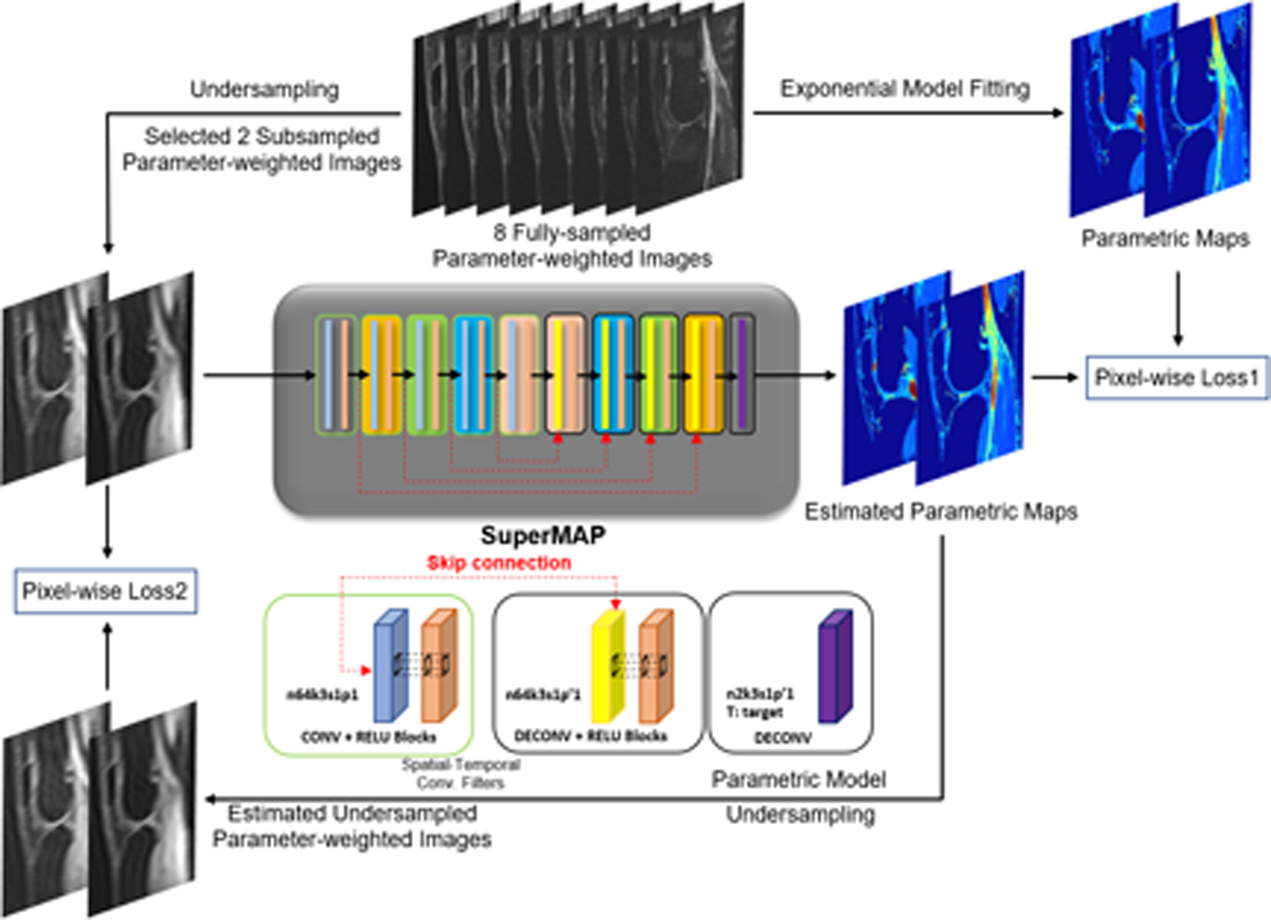
Flowchart of the training process for SuperMAP. The 8 fully-sampled parameter-weighted images are used to generate the training data. SuperMAP network comprises several skip connections to master the residual between input/output. Inside the block, n64k3s1p(p’)1 denotes 64 filters with kernel dimension of 3, stride of 1, and padding (truncation) of 1. The network training uses two losses: Loss1 for the parametric maps and Loss2 for data consistency with the measurement.

In T1rho (or T2) mapping, two undersampled T1rho-weighted (or T2-weighted) images from different spin-lock time (or echo time) are used as the input to generate the T1rho map (or T2 map) as the output. The T1rho maps (or T2 map) from fully sampled, parameter-weighted images are used as the target. During training, the network parameters Θ are learned and updated. In the testing, the newly acquired undersampled parameter-weighted images are fed with learned Θ to construct the desired quantitative maps F(x_t; Θ). SuperMAP exploits both the spatial and temporal correlation among the selected parameter-weighted images while learning the connection from the undersampled weighted images (both in k-space and parameter-space) to the corresponding T1rho (or T2) maps. Some preliminary results have been presented in a conference abstract.⁶²

2.2. SuperMAP for joint parameter estimation

The proposed network can be extended to jointly estimate T1rho and T2 maps from undersampled parameter-weighted images, as demonstrated in Figure 2. With the deep network, 3 contrast images (1^st, 4^th, and 7^th) are used to simultaneously reconstruct both T1rho and T2 maps, where the 1st is a shared contrast image with both T1rho and T2 weighting, the 4^th is a T1rho-weighted image, and the 7^th is a T2-weighted image. The output has 2 channels representing 2 different parameter maps, T1rho and T2 maps. The choice for these 3 contrast images was based on the conclusion drawn from the single-parameter estimation. As shown in Table 2, the use of later contrast images leads to a more accurate estimation. In addition, these 3 parameter-weighted images are undersampled in k-space for additional accelerations. Some preliminary results have also been shown in conference abstracts.^63,64

FIGURE 2.

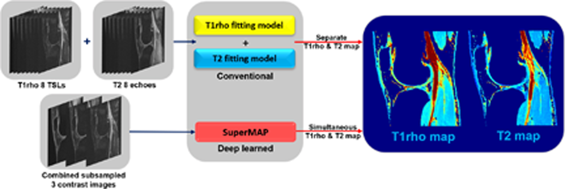
Flowchart of joint parametric mapping using SuperMAP.

TABLE 2.

Quantitative Assessment of T1rho map using different contrast times

TSLs/TEs		1&2	1&3	1&4	1&5	1&6	1&7	1&8
T1rho	PSNR	32.02	33.14	34.22	35.32	36.71	37.17	38.53
	NMSE	0.121	0.101	0.081	0.076	0.045	0.022	0.011
	SSIM	0.94	0.94	0.94	0.96	0.97	0.98	0.98
T2	PSNR	31.32	32.28	33.78	35.02	36.10	37.02	37.30
	NMSE	0.142	0.122	0.095	0.081	0.048	0.024	0.019
	SSIM	0.93	0.94	0.94	0.96	0.97	0.98	0.98

2.3. Patch-based processing

Patch-wise images are utilized in our method. Rather than using the original images, we crop the original images into overlapping patches (size of 21) with an overlapping rate of 67%. Patch-wise processing has several benefits. Small patches instead of an entire image can significantly reduce memory usage, and sufficient training data become available to avoid overfitting, as reported in many studies.^58,59 In this study, there are approximately 6 million training samples from as few as eight in-vivo datasets when using overlapping patches. On the other hand, sufficiently large patches ensure the spatial correlation is learned by the network for enhanced robustness to the aliasing artifacts caused by undersampling, noise, and misregistration due to motion. For a kernel size of three, the patch size is calculated based on the depth of the network (2 × depth + 1).⁵⁸

3. METHODS

3.1. Data acquisition

In vivo full data were collected in compliance with the institutional IRB at a 3T scanner (Prisma, Siemens Healthineers) with a 1Tx/15Rx knee coil (QED). Ten knees were scanned with MAPSS (magnetization-prepared angle-modulated partitioned k-space spoiled gradient-echo snapshots) T1rho and T2 quantification pulse sequence. For T1rho, TSLs were 0, 10, 20, 30, 40, 50, 60, 70 ms, with a spin-lock frequency of 500Hz. For T2, echo times (TEs) were 0, 9.7, 21.3, 32.9, 44.5, 56.1, 67.6, 79.2 ms. For both imaging, matrix size was 160×320×8×24 (PE×FE×Contrast×Slice), slice thickness 4mm, FOV 14cm. Individual coil images were combined using the sum of squares. In addition, two volunteers (four knees) were scanned for prospectively undersampled data collection. The same imaging parameters from the retrospective data were used during the acquisition.

For the single-parameter mapping method, 8 datasets were used to train the proposed SuperMAP and 2 for testing. For acceleration, only the first and the last contrast images (1^st and 8^th) were selected out of 8. The 2D Poisson disk sampling⁶⁵ was used to undersample the phase and partition directions of the 3D k-space retrospectively for further acceleration with an additional acceleration of 2, 3, and 4. For prospective undersampling, 2D Poisson disk sampling was also used with the closest sample to the center of the k-space collected nearest to the preparation pulse of the MAPSS acquisition. We used a Joint Acceleration Factor (J-AF), which is composed of two parts, k-space undersampling and contrast-space undersampling (assuming eight parameter-weighted images are needed to provide a reasonable quantitative map). The parameter maps were generated with joint acceleration factors (J-AF) of 8 (2× acceleration in 1^st and 8^th), 12 (3× in 1^st and 8^th), 16 (4× in 1^st and 8^th), 20 (5× acceleration in 1^st and 8^th), and 24 (6× acceleration in 1^st and 8^th).

For the joint undersampling and reconstruction method, the 1st, 4th, and 7th contrast images were selected. The 1st one was a shared contrast image with both T1rho and T2 weighting, the 4^th was a T1rho-weighted image, and the 7^th was a T2-weighted image. In addition, these 3 parameter-weighted images were further undersampled in k-space to provide additional 2× (J-AF = 10.66), 3× (J-AF = 16), 4× (J-AF = 21.33), 5× (J-AF = 26.66), and 6× (J-AF = 32) accelerations.

3.2. Data processing

Besides using patches, the training dataset was further augmented using image rotations (90 degrees) and image flipping (left/right).

3.3. Network training

During training, a reduced number of undersampled parameter-weighted images are fed as the inputs and the correspondent reference quantitative maps y_i as the targets. Θ is learned through loss function L(Θ) = Loss1 + α Loss2 (2), and the balancing factor α depends on the patch size and the overlapping rate to guarantee the two losses are on the same scale. Loss1 is learned by patch-wise training and Loss 2 is calculated using the entire image. Patches are handled independently and do not need to be put back into the image. To determine α, for example, for an image size of 320 × 320, patch size 21, and an overlapping rate of 67%, there will be approximately 5k patches generated. Then α will be 0.0002 (1 : 5000) to make the Loss 2 on the same scale as Loss 1. In our experiment, the patches are shuffled, which means for a single iteration, the Loss1 and Loss2 do not have to share the same slice as in ordinary cyclic loss in the same batch. By doing this, the model will gain generalizability and robustness. In addition, small patches will improve the computation efficiency (compared to dealing with the entire image).

Euclidean Loss (L2) is used for both losses. The combined loss is minimized by a gradient-based stochastic optimization algorithm ADAM (adaptive moment estimation) implemented in Caffe.^66,67

For single-parameter estimation, the network was trained separately for T1rho and T2 maps. For the combined method, the network for generating T1rho and T2 maps was trained simultaneously. Among the training data, 80 percent were picked as training and the rest 20 percent as validation.⁶⁸ After training, the models can reconstruct the quantitative maps using newly acquired testing data. It is worth noting that both the spin-lock times (TSLs) and echo times need to match between the training and testing data.

The training was achieved using NVIDIA-P6000 × 2 GPUs, with 24GB memory each. The learning ratio was 0.0002 during the first 80 epochs, with 0.9 momentum and decay of 0.0001. For fine-tuning, the learning ratio was reduced to 0.0001 in the following 20 epochs.

3.4. Comparison

Parameter maps from 8 fully-sampled parameter-weighted images using the exponential model fitting were used as the reference maps for comparison. A state-of-the-art deep learning method, MANTIS was also used to reconstruct the T1rho and T2 maps from the datasets with the same undersampling scheme as SuperMAP.

3.5. Evaluation metrics

NMSE (normalized mean squared error), PSNR (peak signal to noise ratio), and SSIM (structural similarity index)⁶⁹ are used to quantify the performance of different methods. Furthermore, coefficient of variations (CV) was calculated for the knee cartilage compartments to evaluate the correlations between the reconstructed T1rho/T2 relaxation times and the references.

4. RESULTS

The training took approximately 10 hours, but only 1 second was needed to generate a complete set of T1rho and T2 maps using the learned network, which is in contrast to the ~3 min processing time for the conventional exponential decay model fitting. The convergence curves for training T1rho, T2, and the joint maps for the J-AF of 16 can be found in Figure S1 (see Supporting Information).

4.1. Single-parameter mapping

Figure 3 shows the T1rho maps from a total of 2 contrast images generated using the proposed SuperMAP and MANTIS. 2D Poisson disk sampling patterns with 2×, 3×, 4×, 5×, and 6× accelerations were used in k-space undersampling within these 2 images. The J-AFs were 8, 12, 16, 20, and 24. MANTIS was used for the J-AF of 16 with the same undersampling scheme for comparison. It shows that the T1rho maps reconstructed by SuperMAP models are closer to the reference and have fewer structured errors than the MANTIS reconstruction, especially in the cartilage region.

FIGURE 3.

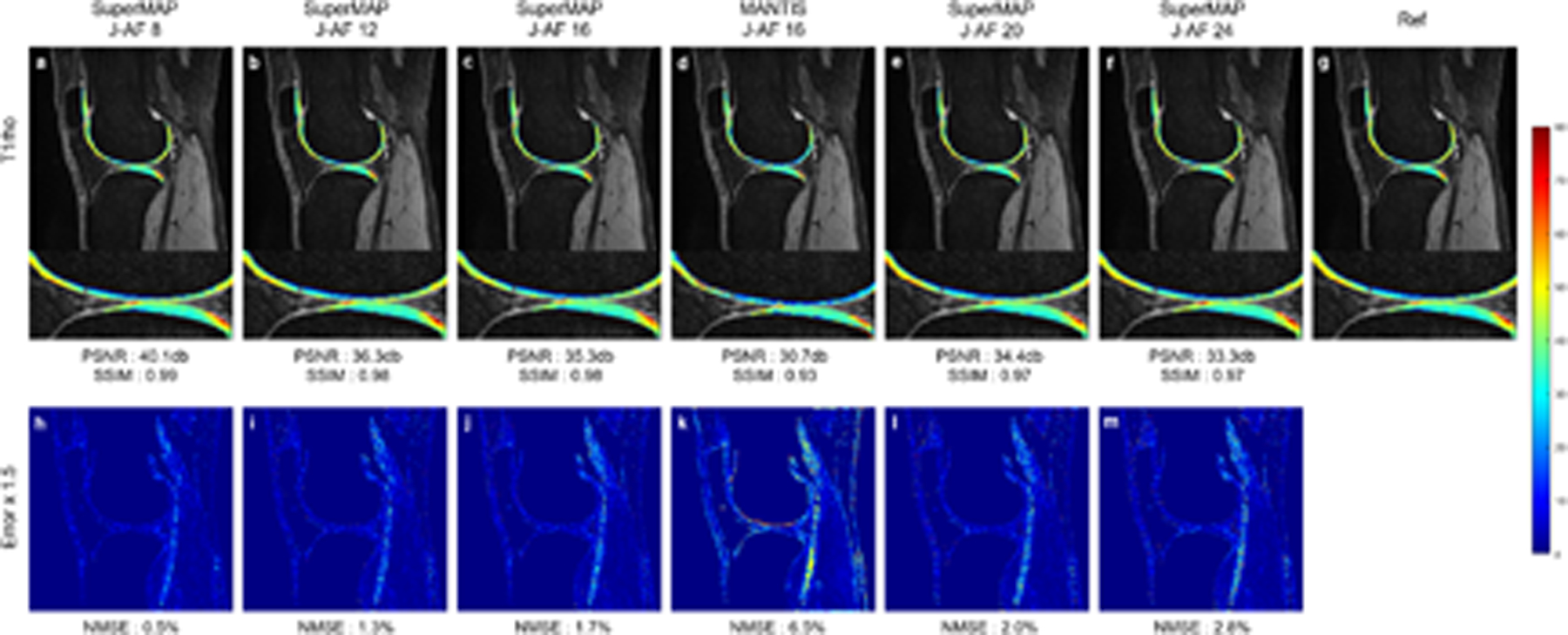
T1rho maps reconstructed from 2 contrast images using SuperMAP with J-AFs of 8 (a), 12 (b), 16 (c), 20 (e), and 24 (f), MANTIS with a J-AF of 16 (d), the corresponding error maps (h)-(m), and reference T1 map (g) from 8 fully-sampled parameter-weighted images.

Figure 4 shows the T2 maps generated using SuperMAP and MANTIS. Same J-AFs as T1rho were used for T2 mapping. Similar observations can be made that SuperMAP is closer to the reference than MANTIS.

FIGURE 4.

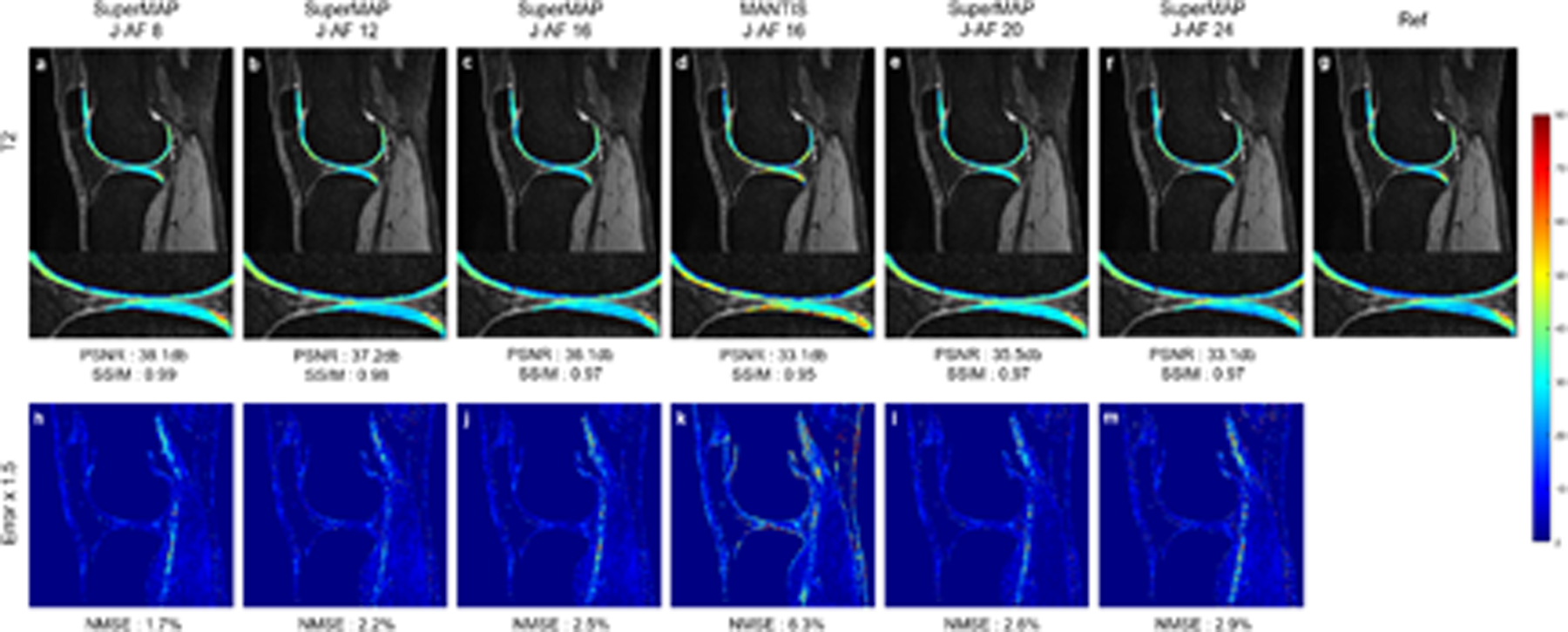
T2 maps reconstructed from 2 contrast images using SuperMAP with J-AFs of 8 (a), 12 (b), 16 (c), 20 (e), and 24 (f), MANTIS with a J-AF of 16 (d), the corresponding error maps (h)-(m), and reference T2 map (g) from 8 fully-sampled parameter-weighted images.

4.2. Joint T1rho and T2 mapping

Figure 5 reveals the simultaneous T1rho and T2 maps using the combined method from a total of 3 contrast images. 2D Poisson random sampling patterns with 2×, 3×, 4×, 5×, and 6× accelerations were used to undersample the k-space of these 3 contrast images. The J-AFs were 10.66,16, 21.33, 26.66, and 32. The quantitative maps generated by SuperMAP were close to the ground truth T1rho and T2 maps, even with only 3 undersampled contrast images. For both single and joint parameter mappings, the PSNRs and SSIMs were shown on the bottom of the reconstructed maps and NMSEs on the bottom of the error maps.

FIGURE 5.

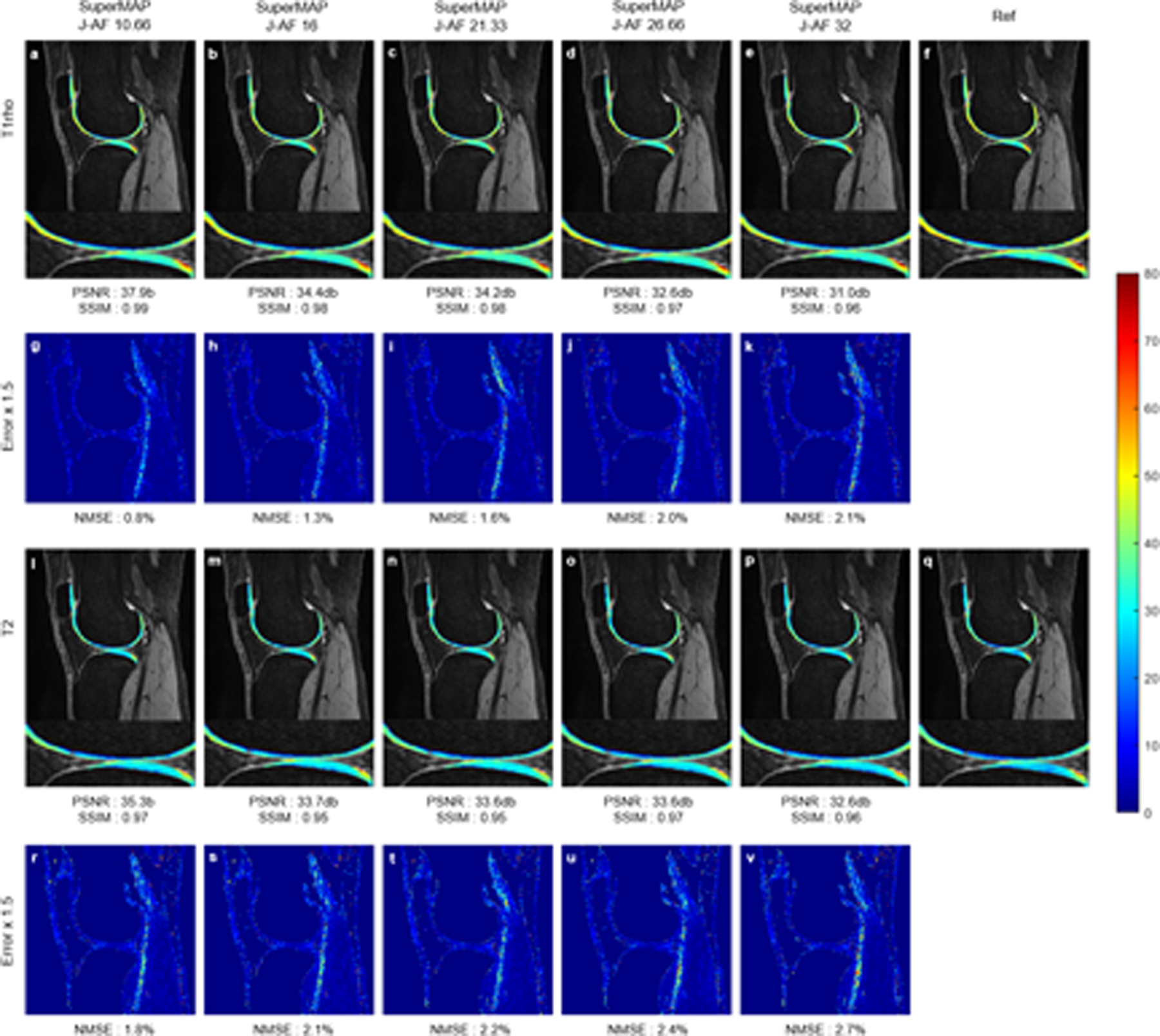
Joint T1rho (top) and T2 (bottom) maps reconstructed from a total of 3 contrast images using SuperMAP with J-AFs of 10.66 (a)(l), 16 (b)(m), 21.33 (c)(n), 26.66 (d)(o), and 32 (e)(p), the corresponding error maps (g-k) (r-v), and reference maps (f)(q) from 8 fully-sampled parameter-weighted images.

4.3. Generalizability test using prospective data

Figure 6 shows the T1rho and T2 maps reconstructed from prospectively undersampled data using SuperMAP with 2 contrast images for single-parameter mapping, and simultaneous T1rho and T2 maps using the combined method from a total of 3 contrast images. Poisson random sampling patterns with 4× accelerations were used to scan. The J-AFs were 16 for the single-parameter mapping method and 21.33 for the joint mapping method. The deep learning models were trained through retrospective experiments with the same undersampling factor and directly evaluated with the prospective data. It can be seen that at slightly lower reduction factors than the retrospective case, the quantitative maps generated by SuperMAP were still close to the ground truth T1rho and T2 maps, further verifying the generalizability of the network.

FIGURE 6.

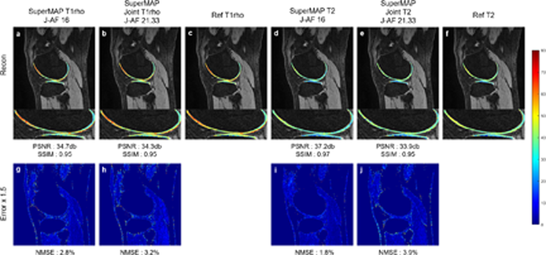
T1rho and T2 maps reconstructed from prospectively undersampled data using SuperMAP with 2 contrast images for single-parameter mapping and 3 contrast images for joint mapping. T1rho (a), Joint T1rho (b), T2 (d), Joint T2 (e), reference maps(c)(f), and corresponding error maps (g-h) (i-j).

4.4. Statistical analyses

One of the test sets was used to evaluate the performance of SuperMAP for T1rho and T2 map estimation with different J-AFs. Quantitative statistics of averaged PSNR, NMSE, and SSIM were summarized in Table 1. The compartment-wise and averaged mean values with standard deviations and the CVs of the independent and joint reconstructions of T1rho and T2 were summarized in Table S1 and S2, respectively. Six cartilage compartments were evaluated, namely, the MFC (medial femoral condyle), the LFC (lateral femoral condyle), the TRO (trochlea), the MTP (medial tibial plateau), the LTP (lateral tibial plateau), and the PAT (patella). The averaged CVs over these six compartments were all below 5% for independent and joint SuperMAP reconstructions with different acceleration factors (except for joint SuperMAP with J-AF of 32). Moreover, SuperMAP outperformed MANTIS at the acceleration factor of 16. Figures S2–S5 depicted the pixel-wise Bland-Altman plots for the proposed SuperMAP methods and the MANTIS method with different acceleration factors. No significant biases were observed in SuperMAP methods.

TABLE 1.

Quantitative Assessment of Separate (SEP) T1rho, T2, and Joint maps using J-AFs

Methods		SEP JAF8	SEP JAF12	SEP JAF16	MANTIS JAF16	SEP JAF20	SEP JAF24	Joint JAF10.66	Joint JAF16	Joint JAF21.33	Joint JAF26.66	Joint JAF32
T1rho	PSNR	41.12	38.95	38.53	32.03	36.55	35.69	41.43	37.70	36.79	35.22	34.16
	NMSE	0.005	0.009	0.011	0.062	0.017	0.021	0.004	0.012	0.016	0.021	0.022
	SSIM	0.99	0.98	0.98	0.93	0.97	0.97	0.99	0.98	0.97	0.97	0.96
T2	PSNR	37.96	37.89	37.30	34.14	37.10	35.17	37.34	36.09	36.08	36.00	35.44
	NMSE	0.016	0.017	0.019	0.057	0.022	0.027	0.019	0.022	0.024	0.026	0.028
	SSIM	0.99	0.98	0.98	0.95	0.97	0.97	0.99	0.98	0.97	0.97	0.96

4.5. Robustness to noise

In practice, the exponential fitting process in parameter mapping needs to be overdetermined to overcome the uncertainty introduced by noise contamination, signal destabilization, hardware imperfections, etc.^46,47 To test the noise robustness, Rician noise (30dB) was added to each parameter-weighted image. As demonstrated in Figure 7, the conventional exponential fitting failed to generate clean T1rho and T2 maps even using all 8 fully-sampled contrast images, as noted in the literature.^46,47,70 On the contrary, SuperMAP can generate accurate maps from 2 noisy undersampled parameter-weighted images, even though the neural network was trained by clean images. The results further demonstrate the advantage of avoiding the model fitting process.

FIGURE 7.

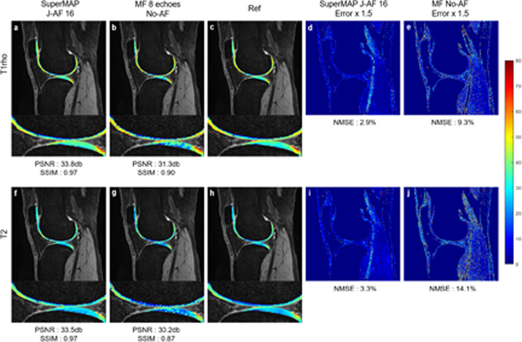
T1rho maps (top) and T2 maps (bottom) reconstructed using SuperMAP from 2 noisy contrast images with additional 4× k-space undersampling (J-AF = 16) (a)(f), from 8 fully sampled noisy data using the exponential model fitting (b)(g), the corresponding error maps (d)(e)(i)(j), respectively, and the reference (c)(h).

5. DISCUSSION

5.1. Contrast selection

With reduced contrast images, different parameter weightings may lead to different maps. Quantitative assessments are summarized in Table 2 for different combinations of 2 TSLs/TEs for T1rho mapping. It reveals that later TSLs/TEs will provide better performance for both T1rho and T2 mapping using our proposed framework. Then we take the combination of the 1^st and 8^th TSLs/TEs as the choice for our experiment. Later TSLs/TEs (corresponds to the 4^th and the 7^th) were also selected for simultaneous T1rho/T2 mapping scenarios. Acquiring 3 TSLs could improve the SNRs and NMSEs, as reported in the conference abstract,⁶² but at the expense of a longer scanner time.

5.2. Training size

The training size was gradually reduced to evaluate the T1rho map reconstructed by SuperMAP with 2 TSLs and a J-AF of 16. As shown in Table 3, both NMSEs and PSNRs remain almost the same until only 1 dataset is used. This result further demonstrates the benefits of overlapping patches.

TABLE 3.

Examination of T1rho map reconstructed by SuperMAP using different training sizes

# of datasets		8	7	6	5	4	3	2	1
T1rho	PSNR	38.53	38.47	38.55	38.42	38.52	38.24	38.11	37.74
	SSIM	0.98	0.98	0.98	0.98	0.98	0.98	0.98	0.97

Table 3 indicates that not many training sets are required to train the proposed network. The 8 training sets used in the study are empirically shown to be sufficient to avoid overfitting and ensure robustness.

5.3. Performance

The results of PSNR, NMSE, and SSIM have demonstrated the superior performance of SuperMAP. In addition, CVs, as another widely adopted metric to measure the dispersion of data from the mean of two methods, have also suggested the clinical applicability of SuperMAP. For instance, Kim et al.⁷¹ recently employed CVs to assess the intra-site repeatability and inter-site inter-vendor reproducibility of a 3D T1rho and T2 imaging sequence on systems from multiple MR vendors. They obtained excellent intra-site CVs ranging from 1.60–3.93% for T1rho and 1.44–4.08% for T2 in human subject knee cartilage.⁷¹ The CVs of the proposed SuperMAP with different acceleration factors fell into the same range, showing promising potential for clinical applications such as the study of osteoarthritis.

6. CONCLUSION

A novel deep learning framework SuperMAP is proposed and evaluated for superfast MR quantitative imaging by undersampling in both k-space and parametric direction. This network incorporates patchwise training with the entire image as the backward cycle (model-data) for consistency. We also present a combined method using SuperMAP to obtain simultaneous T1rho and T2 maps within one scan. For single-parameter mapping, our method can generate T1rho and T2 mapping from as few as 2 undersampled parameter-weighted images. For joint mapping, the T1rho and T2 maps can be simultaneously generated from only 3 undersampled parameter-weighted images. With a scan time of fewer than 1 minute, we can obtain a complete set of T1rho and T2 maps. Optimized undersampling mask, generalizability to different scanners/protocols/patients, and robustness to motion will be explored in future studies.

Supplementary Material

supinfo

FIGURE S1 Training curves for T1rho map (a), T2 map (b), and joint maps (c) for J-AF of 16.

FIGURE S2 Bland-Altman plots for independent T1rho relaxation time reconstruction. (a) to (e) depict the results of SuperMAP method with acceleration factors of 8, 12, 16, 20, and 24 respectively; (f) depicts the result of the MANTIS with an acceleration factor of 16.

FIGURE S3 Bland-Altman plots for independent T2 relaxation time reconstruction. (a) to (e) depict the results of SuperMAP with acceleration factors of 8, 12, 16, 20, and 24, respectively; (f) depicts the result of the MANTIS with acceleration factor of 16.

FIGURE S4 Bland-Altman plots for joint T1rho relaxation time reconstruction. (a) to (e) depict the results of the proposed SuperMAP method with J-AFs of 10.66, 16, 21.33, 26.66, and 32, respectively.

FIGURE S5 Bland-Altman plots for joint T2 relaxation time reconstruction. (a) to (e) depict the results of the proposed SuperMAP method with J-AFs of 10.66, 16, 21.33, 26.66, and 32, respectively.

TABLE S1 Mean relaxation times ± standard deviation (ms) and CVs (in parenthesis) for independent T1rho and T2 reconstructions.

TABLE S2 Averaged compartment relaxation times ± standard deviation (ms) and CVs (in parenthesis) for joint T1rho and T2 reconstruction.