

Abstract

As emerging contaminants, microplastics are challenging to characterize, particularly when their size is at the nanoscale. While imaging technology has received increasing attention recently, such as Raman imaging, decoding the scanning spectrum matrix can be difficult to achieve result digitally and automatically via software and usually requires the involvement of personal experience and expertise. Herewith, we show a dual-principal component analysis (PCA) approach, where (i) the first round of PCA analysis focuses on the raw spectrum data from the Raman scanning matrix and generates two new matrices, with one containing the spectrum profile to yield the PCA spectrum and the other containing the PCA intensity to be mapped as an image; (ii) the second round of PCA analysis merges the spectrum from the first round of PCA with the standard spectra of eight common plastics, to generate a correlation matrix. From the correlation value, we can digitally assign the principal components from the first round of PCA analysis to the plastics toward imaging, akin to dataset indexing. We also demonstrate the effect of the data pretreatment and the wavenumber variations. Overall, this dual-PCA approach paves the way for machine learning to analyze microplastics and particularly nanoplastics.
The demand for plastics in our modern civilization is strong, and the global production of plastics has surpassed 300 million tonnes per year since 2014.1 Due to low recycling rates and poor waste management, unfortunately, an appreciable amount of plastic waste has been released into the environment. The negative effects of minute plastic debris, including microplastics (1–5 mm) and nanoplastics (<1 μm), on aquatic biota, terrestrial plants, and birds have attracted increasing attention over the past decade.2 For human health, despite inadequate evidence on the long-term consequences of ingesting and inhaling microplastics and nanoplastics, some much-needed preliminary data have suggested that these plastic particles and cocontaminants (e.g., additives and toxic compounds attached to the surface of the particles) are likely harmful to human nervous, respiratory, kidney, digestive, and excretory systems.3 It has been estimated that each of us may consume up to 121,000 plastic particles each year.4 These alarming numbers warrant comprehensive research into microplastics and nanoplastics to better understand their sources, fate, risks, and toxicity.
Raman spectroscopy has been recognized as one of the most effective analytical methods to identify and characterize microplastics.5,6 However, analysis of microplastics and nanoplastics with Raman spectroscopy, particularly with Raman imaging, can be difficult due to a number of challenges. First, the Raman imaging usually deals with a large dataset (i.e., a spectrum matrix that contains hundreds or thousands of Raman signal data). To illustrate, scanning an area containing 100 × 100 pixels generates 10,000 sets of spectra, with each set of spectra containing an array of intensity data recorded over a range of wavenumbers (such as −200 to 3700 cm–1). All these hyperspectral data constitute a spectrum matrix containing multiple dimensions (intensity, wavenumber, and spatial coordinates). The high degrees of dimensionality often spell trouble for the extraction of important microplastic information. Second, spontaneous Raman scattering is commonly weak and thus places a limitation on the intensity of the collected signal data.7 This inherent weakness of the signal underscores the importance of enhancing the signal-to-noise ratio, such as by decreasing the spectrum background, particularly for environmental samples. Third, sample preparation for Raman analysis can be complicated. Isolating target particles from environment constituents is a demanding task, often leading to inadequate removal of interferences (e.g., certain organic matter and particles).8 Moreover, the coexisting ingredients in the plastics, such as pigments or dyes, biofilms formed on the plastic surface, and derived surface groups due to weathering/aging, may create a hindrance to the comprehension of the Raman data through considerably modifying Raman spectra or completely masking polymer signals.9
Several methods can be used to enhance the effectiveness of Raman analysis. For example, improving the setup of a Raman spectrometer through the optimization of optical structure was demonstrated to significantly increase the signal-to-noise ratio.10 A number of sample preparation techniques were also considered to raise the signal quality.8,11 Data interpretation is another critical aspect. In comparison with the data from a single Raman spectrum, the large matrix dataset generated by Raman imaging by its nature offers an increased signal-to-noise ratio, from a statistical point of view.12 In recent decades, data processing using chemometrics has attracted increasing attention to decode and analyze the complicated spectrum matrix toward automation and machine learning.13,14
Multivariate statistical techniques applied in chemometrics are known to be powerful tools to decode the multidimensional Raman spectrum matrix.15 Various data mining chemometrics are available nowadays, and principal component analysis (PCA) is a potentially suitable algorithmic option to decode the Raman spectrum matrix.16 In principle, PCA works by reducing a large number of variables to a much smaller set of orthogonal principal components that reflect the variations in the dataset to a greatest extent. As a result, the dimensionality is reduced considerably, while the relevant information is retained.17 Through determining the number of principal components and creating principal component score/loading curves (so-called PCA spectra/intensities) to mimic Raman spectra, the major spectrum information can be extracted.18
In order to increase the accuracy of the PCA analysis, prior to the PCA calculation, data preprocessing is commonly essential. The data preprocess can effectively and intentionally remove the background noise and the irrelevant intensity variation.19 Furthermore, after the PCA analysis, principal components can sometimes be difficult to interpret. Consequently, the assignation of PCA spectra to certain chemicals cannot be conducted automatically, but compared with the standard Raman spectrum and justified by the naked eye according to personal experiences.18 Therefore, an additional step, such as by a subsequent algorithm analysis or by packaged software, is preferred to facilitate the initial PCA analysis. Putting together preprocessing, the initial PCA, and the resultant analysis, a Raman spectrum can be automatically and digitally analyzed, which is a further step toward machine learning.13,14,20
In this work, we aim to improve a PCA-based algorithm that we reported earlier,18 to enhance the extraction of important information from the Raman spectrum matrix. First, several data pretreatment methods are employed, including baseline correction, wavenumber range selection, curve smoothing, and cosmic ray removal. Then, we apply a dual-PCA process that involves (i) an initial PCA analysis (first round) to create the PCA spectra and generate the PCA intensity images and (ii) a second round of PCA, by combining the PCA spectra created in the first round of PCA with eight standard spectra of the common plastics, to automatically and digitally assign the principal components (of the first round of PCA) to the suspected items via the correlation matrix (of the second round of PCA), akin to an index.21 To validate the effectiveness of this improved method, we test it first on a mixture of two virgin microplastics and then on a sample collected during lawn trimming in our gardens. The results from this study might be useful in facilitating the development toward machine learning for the analysis of microplastics and little-known nanoplastics.
Experimental Section
Microplastics
All virgin microplastics (beads or pellets, usually with diameters <1 mm), including polystyrene (PS), polyethylene terephthalate (PET), polyethylene (PE), polyvinyl chloride (PVC), and polypropylene (PP), were purchased from Sigma-Aldrich (Australia) and used as received unless further indicated. Several Raman spectra were extracted from the database when the standard plastic samples were not available, inducing polyamide (PA or PA 6), poly(methyl methacrylate), and polycarbonate (PC, be careful, it is different from the principal components of PCA, marked as PC# in this study, such as PC1, PC2, etc.).
Sample Preparation
A microplastic mixture including PE and PVC was selected as a model to validate the algorithm analysis.22 Basically, equal amounts (in volume) of PE and PVC were mixed together in a mortar that was previously cleaned with Milli Q water and ethanol. The microplastic mixture was then uniformly distributed on a glass slide for the Raman test.
A trimmer was operated to mimic mowing in our garden.23 We used an aluminum tray to collect the trimmer line debris. In the tray, we used a glass slide to mimic the concrete curb, soil, and grass. The trimmer line was gradually touched down onto the glass slide, like normal use, for several seconds (be careful not to break the glass to release small sharp pieces!), for the trimmer line to scratch and mark the glass surface. The scratches on the glass slide were directly tested by Raman.
During the sample preparation process, suitable personal protective equipment should be worn, including a pair of glasses to protect our eyes. Denim jeans, jacket, cotton gloves, and boots are recommended as well.
Raman Analysis
Raman spectra were recorded in air using a WITec confocal Raman microscope (Alpha 300RS, Germany) equipped with a 532 nm laser diode (<30 mW), as reported previously.11,22,24 A charge-coupled device (CCD) detector was cooled at −60 °C to collect Stokes Raman signals under a 20× or 100× objective lens at room temperature (∼24 °C).
To map an image, the stage-moving speed (controlled by a piezo-driven scanning stage) for each Raman signal collection at each pixel was varied, from 1 × 1 μm to scan an area of 88 × 88 μm with 88 × 88 pixels, to 0.33 × 0.33 μm to scan an area of 10 × 10 μm with 30 × 30 pixels, as indicated below. The Raman scanning duration was changed accordingly. In the former case, it was 7744 s (88 × 88); in the latter case, it was 900 s (30 × 30), where each pixel takes 1 s to collect the Raman signal.
For Raman image mapping, the sample was scanned using a 20× or 100× objective lens. The different plastics exhibit different Raman activities and emit different intensities of Raman spectra, as suggested previously.22 For image mapping, we select the characteristic peak that should be strong and not overlapped with the peaks of the other plastic. For example, the Raman signal at 1059 cm–1 was picked up to image the PE, along with other characteristic peaks (1130, 1300, and 1450 cm–1). The intensities at different peaks were mapped as different colors of images.
Image Analysis: Logic-Based Algorithm
The collected Raman signal was analyzed using WITec Project software. By only picking up the net intensity of their characteristic peaks for image mapping, the interference that might originate from the background as noise (such as fluorescence) or organic matter can be effectively and intentionally avoided by subtracting the baseline of the collected Raman spectra to obtain the net intensity (the peak area or sum, after automatic integration via software). That is, the spectrum background has been intentionally subtracted using the collected signal at both sides of the selected Raman peak at the pixels as the background. To further avoid the “bias and false” imaging, a logic-based algorithm analysis is recommended.
From the Raman spectrum matrix, several images were simultaneously mapped at different peaks, such as for PE at 1059, 1130, 1300, and 1450 cm–1. At these peak positions, the intensity signal can be mapped in different colors. Two or more images, which correspond to two or more different characteristic peaks, can be merged, either by logic-OR, logic-AND, or logic-SUBTRACT, as reported previously.12,24
In the case of “logic-OR,” any mapped signal at each pixel from the “parent images” will be picked up and merged into a new image (daughter image). Obviously, any “bias and false” noise from the parent images (mapped at two different Raman peaks) might be picked up. In the case of “logic-AND”, only the signals at the same pixel that simultaneously appear in both of the parent images can be picked up in a new “daughter image.” While some signal might be lost, the noise is also expected to be reduced in the daughter image. These algorithms can be combined and mixed to analyze the “parent images”, to generate a “daughter image”, a “granddaughter image”, or even to generate an “offspring image” etc.
For the logic-based algorithm analysis, the ImageJ software was employed. In general, the parent Raman images are opened by the software and converted from the RGB to 8-bit format. Then, the images are processed and merged with a calculator of logic-OR or logic-AND. Another option for logic-OR is conducted via color-merge-channels. After merging, the new image is painted to the selected color in the displaying value range of 0–30 (adjustable and depends), which can be converted back to the RGB format as the daughter image. These daughter images can be further analyzed with the algorithm.
Data Analysis: PCA-Based Algorithm
The raw data from the Raman scanning were analyzed by PCA in Origin (Pro 2020) software. For our Raman setup, it generally exports the Raman intensity data at 1028 individual wavenumbers. The exported raw data of Raman intensity were then imported to Origin, so that each row contains the Raman signals at the same individual wavenumber, and each column contains a whole set spectrum at different wavenumbers. Consequently, in a data matrix, the total number of the rows is 1028, while the total column number is the number of pixels from the scanning array, which depends on the size of the pixel and the scanning area/array. That is, each set of Raman spectrum has been collected at each pixel, the number of which (pixel or column) is 88 × 88 or 30 × 30 in this study.
To excite the Raman emission, a laser was employed. To collect the Stokes Raman signal, a filter is generally used to remove the laser. Even so, some laser residues survive the filtration, to be collected and mixed with the Raman signal. To remove this part of interference, we intentionally remove the signal <200 cm–1, prior to the PCA analysis, as discussed below. More spectrum pretreatments are also indicated below.
All of the pretreated data, excluding the wavenumber (or wavelength) that can serve as the “observation label” or can be removed from the data matrix but linked with the row sequence number, participated in the PCA analysis, under the parameters such as “correlation analysis”, “exclude missing values of listwise”, “quantities of compute including eigenvalues and eigenvectors”, etc. The principal component number (PC#), or the number of components to extract, was adjusted according to the estimation of how many items or suspects could be located in the scanning area. Usually, five principal components are enough.
After PCA, a scree plot, loading plot, and score plot were provided. The principal component score, related to the individual principal component, was combined with the Raman wavenumbers (via the row sequence number of the data matrix) to regenerate a curve, labeled as “PCA spectrum”, to mimic and compare with the Raman spectrum. These mimicked curves were compared with standard Raman spectra, if available, to allow identification of plastics and other suspected items.
The coefficients of the principal components, the extracted eigenvectors, were combined with each mapping pixel’s position of the scanning array (via the column sequence number of the matrix) to map the images, the “PCA intensity images”. The principal component loadings can also be used for the image generation. Similarly, the mean and the standard deviation of the descriptive statistics can also be mapped as images. When the principal component number is higher than three, only selected dimensional plots are presented due to the presentation limit of the highest dimension of three.
The raw data of the Raman spectrum matrix can be transposed for each row to contain a set of spectra. In this case, the principal component loading will generate the PCA spectrum to mimic the Raman spectrum, while the principal component scores will be mapped as the PCA intensity images.
Results and Discussion
Effect of Spectrum Pretreatment, Prior to PCA
To enable an accurate PCA analysis to identify microplastics efficiently, the raw spectrum can be pretreated. By doing so, not only the noise can be effectively removed, but also the biases can be significantly decreased. In Figure 1a, the unprocessed Raman spectrum has a strong background, which might originate from the pigment/dye or other additives in the plastic material, or from the derivate surface groups due to weathering/aging, or from the accompanied components such as biofilms surviving the sample pretreatment.25 Being considerably more intense than Raman scattering, the background can shield the Raman signal. As a result, the subsequent PCA likely yields nonessential results by recognizing the background signal variations as dominant principal components.26 It is thus important to correct the baseline and minimize nontarget fluctuations in the Raman signal.20 To remove the background, we used asymmetric least squares, with the following parameters: asymmetric factor, 0.001; threshold, 0.05; smoothing factor, 6; number of iterations, 10; and so on. After the baseline correction to remove the spectrum background, the spectrum looks better.
Figure 1.

Pretreatment of the Raman spectrum, including (a) baseline correction, (b) wavenumber range selection, (c) curve smoothing, and (d) cosmic ray removal. In (d), two spectra are pretreated to remove the cosmic rays (arrowed).
To excite the Raman, we need a laser. Due to the laser’s reflection or Rayleigh scattering, the Raman emission is mixed with the residue laser. As Raman scattering intensity is often weaker than Rayleigh scattering intensity,27 this residue laser should also be removed, as shown in Figure 1a,b. When we delete the signal <200 cm–1 (not the fingerprint range) and subject it to background correction, the baseline in the low wavenumber range is flatter than that in Figure 1a, as circled in Figure 1b. Similarly, we can also cut off the signal at the high wavenumber range that does not contain plastic signal, such as >3500 cm–1, to standardize it in the same wavenumber range for comparison. By doing so, any significant unwanted variations outside the selected wavenumber range can be circumvented, facilitating the PCA identification of key chemical information.
When the Raman signal is weak, the variation of the Raman signal is significant and usually presents as a random noise, as observed in Figure 1a,b. This kind of random noise (not the spectrum background) may result from two main sources, including the CCD detector (dark current and reading noise) and the signal itself (shot noise); the impact of noise can be strong under certain circumstances, such as short integration time or use of a high wavelength laser.28 The noise can be hopefully removed by smoothing. The result is shown in Figure 1c. Herewith, we select an adjacent-averaging mode with the points of window of 5. Consequently, the signal-noise ratio can be increased.
Sometimes, cosmic rays are collected with the Raman signal.29 Cosmic rays are randomly generated and result from decay of radioactive atoms present within the CCD detector, which is known to distort the principal component direction in PCA.30 They should be removed before the PCA analysis, particularly when the Raman spikes caused by cosmic rays overlap the characteristic peaks, as presented in Figure 1d. Here, we selected two spectra as examples. We used (i) a percentile filter (points of window, 5; boundary condition, none; and percentile, 50) and subsequently an FFT filter (points of window, 5) to remove the cosmic rays. After filtration, cosmic rays can be significantly decreased, if not completely removed.
Not all of these pretreatments are compulsory and positive for analysis. For example, depending on the pretreatment algorithm and the signal-noise ratio of the raw spectrum, some pretreatment might lead to the signal loss, such as when over-conducting the baseline correction and over-smoothing the curves. From our current experiences, we generally recommend the pretreatment of the wavenumber range selection and the cosmic ray removal, prior to the dual-PCA analysis. Caution should be exercised in the use of other pretreatments, depending on the raw data.
Dual-PCA: A Mixture of Two Virgin Microplastics
As reported recently, when a sample surface is scanned, we can map the specific molecular spectrum to visualize the sample by generating an image.22 During this scanning process, a spectrum matrix, akin to a hyperspectral database, is produced. To decode this matrix toward imaging, PCA has been demonstrated to enable effective extraction of spectrum information.13,14,18 Ideally, PCA can decompose the spectrum matrix to two new matrices, one containing the spectrum profile to enable the identification of the target and another containing the spectrum intensity to map the image.
Herein, we test a “known” sample first,22 which is a mixture of virgin PVC and PE. After cutting off the wavenumbers to focus on the wavenumber range of 200–3500 cm–1 and removing the cosmic rays, the PCA can extract the several main principal components. Their loading coefficients are mapped as images and shown in Figure 2.
Figure 2.
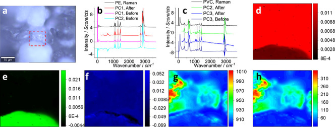
First round of PCA analysis on the Raman spectrum matrix, including a (a) photo image, (b,c) PCA spectra, and (d–f) PCA intensity images mapping the loading coefficients of PC1–PC3, respectively, the (g) mapped mean, and (h) standard deviation. In (a), the squared area 88 μm × 88 μm was scanned to collect the Raman signal with a pixel size of 1 μm × 1 μm, 0.5 s integration, to generate a spectrum matrix containing 7744 (88 × 88) sets of Raman spectra. In (b,c), the Raman spectra of PE and PVC are presented for comparison, with the characteristic peaks marked with dashed lines, after intensity off-setting. The PCA analysis was conducted “Before” and “After” the raw data from the spectrum matrix were subjected to pretreatment, as marked. The images in (d–h) are generated from the PCA analysis after the spectrum pretreatment.
In Figure 2a, there are several particles. The squared area contains two particles that were assigned to PVC and PE, as confirmed and reported before (Figures S1 and S2, Supporting Information).18,22 Herein, we pretreated the raw data and subjected the spectrum matrix to the PCA analysis. Accordingly, more accurate analysis results are obtained here and marked as “After” (compared to “Before” the pretreatment). In Figure 2b,c, for the PCA spectra of “After”, according to characteristic peaks that are marked with dashed lines, we can assign PC1 to PE and PC2 to PVC, which is different from “Before” when we assigned PC1 to background/PE, PC2 to PE, and PC3 to PVC, respectively.18 This can be mainly attributed to the removal of the undesirable Rayleigh scattering signal in the low-frequency region.31 The result suggests the importance of selecting an appropriate wavenumber range.
When the loading coefficients of principal components are mapped as images, Figure 2d–f is generated, which is also different from “Before” (Figures S1 and S2, Supporting Information). Herein, after the pretreatment, the clear patterns of PE and PVC are mapped in (d,e), directly and certainly, without interference from each other, suggesting the improvement of the PCA analysis.
Another image in Figure 2f (and Figure S2, Supporting Information) resembles the noise or the calculation variation, as we cannot distinguish the patterns of PVC and PE. Although the PCA spectrum of PC3 in Figure 2c is somewhat comparable to that of PVC, the proportion of variation explained by this eigenvalue (0.23%) is much lower than that of PC2 (16.73%) and PC1 (81.59%). Consequently, it is difficult to distinguish the PE from PVC in the mapping image in (f).
The mapped mean (g) and deviation (h) enable visualization of the distribution of the main signal collecting area and the analysis uncertainty area. That is, from Figure 2g, we can see that the signal is stronger in the top-half area than in the bottom-half, mainly from PE. However, in this top-half area, the analysis standard deviation is also higher in (h). This is because the confocal Raman is focused on the top-half part so that the signal over this part can be more efficiently collected. Another possible reason is that, for this sample, the Raman activity of PE is higher than that of PVC.
In Figure 2a, only parts of the two particles in the area have been squared and scanned. In Figure 2d, once the top-half is assigned to PE, the assignment can be reasonably expanded to the whole item connecting this scanned area in (a). Similarly, in Figure 2e, the same expansion can be conducted for the bottom-half. We thus can assign the whole particle in Figure 2a in the middle part to PE, and the bottom particle to PVC.14 Note that the precondition for this assignment expansion is that each particle is made of the same plastic, uniformly.
Although we can generate images to visualize the distribution of the two microplastics, we need Figure 2b,c to compare the PCA spectrum with the Raman spectrum, using the naked eye for the assignment. This kind of assignment has limits and may create some bias. That is because, in Figure 2b,c, the comparison is not straightforward, even after the improved PCA analysis. In the following, we will develop a method to conduct the comparison and assignment automatically and digitally, via a software algorithm, rather than via the naked eye. The personal bias or human error can thus be significantly decreased, if not completely overcome.
The five decoded PCA spectra from the first round of PCA analysis are presented in Figure 3a. Figure 3b compares three of them with the standard Raman spectra of plastics, which include eight common plastics that we usually use in our daily life. As mentioned in Figure 2b,c, the vision-based comparison is complicated, even with the dashed lines to indicate the characteristic peaks of each plastic (PE or PVC). In Figure 3b, when the three PCA spectra are compared with eight Raman spectra, the situation is much more complicated, and an algorithm approach is thus preferred. An algorithm-based comparison is to recognize a digital value to indicate the similarity or difference, among a suspected spectrum and the standard spectra, akin to an index.21 Fortunately, the correlation of PCA analysis can be used for this comparison and justification.
Figure 3.
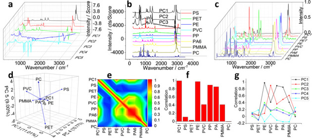
Second round of PCA analysis on the first round of PCA spectra of PC1–PC5 in Figure 2. (a) shows the PCA spectra extracted from the first round PCA analysis. (b) PCA spectra of PC1–PC3 and comparison with standard Raman spectra of eight common plastics, after intensity off-setting. (c) Pretreated spectra in (b) for the second round of PCA. After the second round of PCA analysis, the (d) loading plot, the (e) correlation matrix, and the (f) correlation value of PC1 (of the first round PCA) are shown. (g) Results of the correlation value of PC1–PC5, when they are individually subject to the second round of PCA analysis.
Taking the PCA spectrum of PC1 from the first round of PCA for example, we compare it with the eight standard spectra, in order to identify the type of plastic.21 To avoid the comparison bias and to increase the accuracy, we pretreat the spectrum, as discussed above. The pretreatment includes the baseline correction, smoothing, and cosmic ray removal, interpolating to adjust the wavenumber (x axis) and normalizing the intensity (y axis). After the pretreatment, the spectra are presented in Figure 3c.
We then run a second round PCA analysis on this spectrum matrix that contains one PCA spectrum and eight Raman spectra. From the loading plot in Figure 3d, we can see that the main eight plastics can be effectively separated and distinguished from each other, which enables the assignment of a suspected sample to one of those plastics. Due to the presentation limitation, herein, only a three-dimensional plot of PC3–PC4–PC5 (of the second round of PCA) is shown (as x–y–z axis), and the rest are shown in Figure S3 (Supporting Information). In this three-dimensional plot, PC1 (of the first round of PCA) looks close to PE toward allocating its assignment.
As discussed above, we run this second round PCA in order to extract a new matrix, the correlation matrix, although there might be other options and algorithms to obtain the correlation as well. The data are shown in Table S1 (Supporting Information) and imaged in Figure 3e. The “sword” shape matrix is dominated by the spectra of eight plastics and is symmetrical along the diagonal. Only the top part (or the left part) is contributed by the PCA spectrum of PC1 (of the first round of PCA). We thus extract this part of information and present it in Figure 3f. While the “sample of PC1” has a correlation of “1” for itself, it yields the correlation values of 0.9804 with PE, 0.8954 with PP, and 0.85268 with PA. If we set a threshold value of 0.9 or take the maximum, we can assign PC1 to PE, which agrees with the vision-based justification in Figures 2b/3b, suggesting the success of the digital assignment.
Similarly and in parallel, we combine each of the PCA spectrum of PC2, PC3, PC4, and PC5 from the first round of PCA and run the second round of PCA individually. We then extracted their correlation values for comparison, and they are listed in Figure 3g. Again, if we set a threshold value of 0.9 or take the maximum, we can assign PC2 to PVC, similar to the assignment of PC1 to PE. The correlation values of others are low, all <0.4. Therefore, we assign them to noise, rather than plastics.
This digitalized assignment from the PCA correlation value of the second round of PCA in turn can support the assignment of the mapping images in Figure 2. The mapped images of the loading coefficients of PC1 and PC2 are thus to visualize the distribution of microplastics, including PE and PVC, while the rest are assigned to the noise or background.
The above analysis is for a sample that we tested before and we know that it is a mixture of PE and PVC.18,22 In the following part, we will validate this dual-PCA approach to analyze an “unknown” sample.
Dual-PCA: An Unknown Sample for Validation
When we use a trimmer in our garden, we might generate nylon microplastics, or more seriously, nanoplastics.23 For comparison with our new approach of dual-PCA, Figure 4 shows the results when a previous approach is employed to generate images.12,22 We extract the Raman peak intensity at the characteristic peaks of the nylon and map them as images.
Figure 4.

(a) Photo image, (b) typical Raman spectra, and (c–j) intensity images mapped at characteristic peaks of PA6/nylon, as indicated under the images (with the peak width as well). The photo image of 10 μm × 10 μm in (a) was scanned, and all Raman signals were collected with a pixel size of 0.33 μm × 0.33 μm, 1 s integration, to generate a matrix containing 900 (30 × 30) sets of Raman spectra. In (b), the spectrum of PA6 is presented and compared with three typical spectra collected during the scanning process, a relatively strong one, a middle one, and a weak one. For images (c–j), the color off-setting of 10% is carried out to pick the strong intensity at the different peaks, except in (d), where the spectrum background has not been removed. (j) is an image merged (c, e–i), using logic-OR/AND, as suggested.
Figure 4a shows the photo image. We can hardly see and assign nanoplastics, either due to light diffraction, the resolution of the camera, or the absence of the molecular information. Raman spectra are shown in Figure 4b, which were collected during the scanning process. There are three typical spectra, one with a relatively strong signal, one of middle strength, and one that was collected from the blank area as the spectrum background. Basically, all the Raman signal is weak.
When mapped at the characteristic peaks of nylon, images (c–j) are generated. We can see that the mapped pattern is well matched with that in Figure 4a. However, most of them are blurry, so the image certainty is low, due to the contribution from the individual peak of the spectrum, rather than from the whole set of spectra. If we did not remove the spectrum background, the image in Figure 4d actually shows a clear pattern. However, the molecular information is uncertain, due to the presence of the background. When the individual images are merged together for cross-checking and to increase the signal-noise ratio, the image (j) gets more blurry, except the bright dot (500–800 nm) at the right-bottom corner. The logic-based algorithm is limited in its ability to increase the assignment certainty, particularly when the signal is weak and when the item size is at the nanoscale. The noise dominates the images, as shown here.
In order to map an image with a higher certainty or signal-noise ratio, we run the first round of PCA to decode the spectrum matrix to map the PCA intensity images and simultaneously generate the PCA spectra,18 and the second round of PCA to assign the suspected materials, digitally and automatically, after merging the PCA spectrum with eight plastics’ standard spectra. The results are shown in Figures 5/6.
Figure 5.

Results of the first round of PCA analysis on the raw Raman data presented in Figure 4. (a) PCA spectra of PC1–PC5 and comparison with the Raman spectrum of PA6, after intensity off-setting. (b–d) Images mapping the loading coefficients of (b) PC1 and (c,d) PC2, respectively. (d) Another version of (c), using a three-dimensional presentation.
Figure 6.

Results of the second round of PCA analysis on the raw Raman data presented in Figures 4 and 5. Taking PC2’s PCA spectrum (of the first round of PCA) as “Sample”, and subjecting it to the second round of PCA analysis, (a) shows the loading plot, (b) correlation matrix, and (c) correlation values.
Figure 5 shows the results after the first round of PCA analysis. We extract the PCA spectra and show them in Figure 5a. When compared with the standard Raman spectrum of nylon (PA6) via the naked eye, we can suspect PC2 to be nylon, PC1 to be the spectrum background, and PC3–PC5 to be noise. The mapped images are shown in Figure 5(b–d), including the loading coefficients of PC1 and PC2. The images mapping other coefficients, the mean, and the standard deviation are shown in Figure S4 (Supporting Information).
We then run the second round of PCA analysis in order to assign the suspected items digitally.
Figure 6 shows the results after the second round of PCA analysis. Again, we merge the PCA spectrum of PC2 (named as “sample”) with the eight common plastics, as shown in Figure 3c. After the pretreatment, including baseline correction and smoothing, interpolation, and normalization, we run PCA analysis again. Similarly, we also show the loading plot in Figure 6a, using a three-dimensional presentation including PC3, PC4, and PC5. It looks like our sample is close to PP and PA.
The correlation matrix is shown in Figure 6b, and the data are shown in Table S2 (Supporting Information). When extracted from the matrix, the correlation value of “sample” is shown in Figure 6c. The highest value of correlation is 0.95339 for nylon of PA followed by 0.91139 for PP and 0.88269 for PE. The higher correlation value yields a higher certainty, which leads us to assign it to PA. We thus recommend that the maximum correlation value should be taken. More research is needed here to broaden the database and to cover more types of plastics. In addition to the polymer information, the spectra of comment coingredients, such as colorants and plasticizers,32 can also be added to the database.
The assignment to PA can be used in the images in Figure 5b,c, to visualize the distribution of PA including a wire (diameter or width <1 μm) and a nanoplastic (size <1 μm),5,33 with a much higher certainty and clarity than that in Figure 4, suggesting the advantage of this dual-PCA approach. In Figure 5d, we even can see an extra weak fragment or particle that is mapped with a low PCA intensity. Note the intensity image is not directly related to the physical size along the z axis direction, no matter whether it is microplastic or nanoplastic. That is, this dual-PCA can effectively pick up the strong signal, along with the weak signal, and map them in the x/y axis plane.
Effect of Wavenumber Variation
Another advantage of this dual-PCA approach is that the variation of the wavenumber/wavelength has a very limited effect on the assignment, as shown in Figure 7. Wavenumber variation can be caused by instrumental or measurement environmental changes.34 Different detectors of the Raman setup to collect the Raman signal can suffer from this kind of variation, either due to the prism/transform issue or owing to the wavenumber resolution and the measurement shift etc. Furthermore, the change to the measurement environment (e.g., from the solid phase to aqueous phase, to the adsorbed phase35) and the change to the chemical bond situation (such as electronic structure, geometric isomerism, and molecular conformation36) might shift the position of the peaks too. In the meantime, the temperature fluctuation may also cause wavenumber drifts at a rate of ∼0.1 to 0.4 cm–1/°C.37 From our experiences of using different brands of the Raman setup, also echoed by the literature report,35 this kind of wavenumber variation might be as high as 10–20 cm–1, even when the wavenumber calibration has been conducted prior to each test. This is the reason why in Figure 7a we intentionally shift the wavenumber to a lower range of down to −10 cm–1, or to a higher range up to 10 cm–1, to demonstrate the effectiveness of our dual-PCA method. Note that herein only partial spectra are shown, but the whole set of spectra has participated in the dual-PCA analysis.
Figure 7.

Variation of the (a) wavenumber and the effect on the (b) correlation value.
Fortunately, after the dual-PCA analysis, the values of the correlation are still located within an acceptable range. If we assign the suspected item via the maximum value, there is no change for us to assign it to PA again, as suggested in Figure 7b. The correlation values are listed in Table S3 (Supporting Information). Despite this positive result, more research is needed to better understand the robustness of the dual-PCA method in response to spectral changes.
Conclusions
We successfully demonstrated a digital approach to enable the identification and assignment of plastics, via two rounds of PCA analysis. This paves the way for machine learning to analyze the microplastics and particularly nanoplastics.
Before the analysis process demonstrated in this research can been implemented as a software package, we need more research to address several challenges, including (i) the involvement of the Raman scanning process, to enable the specific area to be selected for position/item-intentional scanning, prior to the analysis, or for in-situ feedback from the PCA analysis; (ii) a more accurate decoding in the first round of PCA analysis to extract more meaningful information; (iii) the involvement of more plastics to take part in the second round of PCA analysis, even including some other items such as dyes/pigments etc. from a universal database; and (iv) combination with some supervised algorithms to finally realize a machine learning process.
Acknowledgments
The authors appreciate the funding support from CRC CARE and the University of Newcastle, Australia. For the Raman measurements, we also acknowledge the use and support of the South Australian node of Microscopy Australia (formerly known as AMMRF) at Flinders University, South Australia, and the Key Lab of Urban Environment and Health, Institute of Urban Environment, Chinese Academy of Sciences, Xiamen 361021, P. R. China.
Supporting Information Available
The Supporting Information is available free of charge at https://pubs.acs.org/doi/10.1021/acs.analchem.1c04498.
Author Contributions
The manuscript was written through contributions of all authors. All authors have given approval to the final version of the manuscript. The authors Cheng Fang, Xian Zhang, and Ravi Naidu were involved in experiment design and management. The authors Cheng Fang and Zixing Zhang participated in data collection and sample preparation. The author Yunlong Luo and Zixing Zhang helped the manuscript preparation and reviewing process.
The authors declare no competing financial interest.
Supplementary Material
References
- Lebreton L. C. M.; van der Zwet J.; Damsteeg J.-W.; Slat B.; Andrady A.; Reisser J. Nat. Commun. 2017, 8, 15611. 10.1038/ncomms15611. [DOI] [PMC free article] [PubMed] [Google Scholar]
- Eerkes-Medrano D.; Thompson R. C.; Aldridge D. C. Water Res. 2015, 75, 63–82. 10.1016/j.watres.2015.02.012. [DOI] [PubMed] [Google Scholar]
- Campanale C.; Massarelli C.; Savino I.; Locaputo V.; Uricchio V. F. Int. J. Environ. Res. Public Health 2020, 17, 1212. 10.3390/ijerph17041212. [DOI] [PMC free article] [PubMed] [Google Scholar]
- Cox K. D.; Covernton G. A.; Davies H. L.; Dower J. F.; Juanes F.; Dudas S. E. Environ. Sci. Technol. 2019, 53, 7068–7074. 10.1021/acs.est.9b01517. [DOI] [PubMed] [Google Scholar]
- Gigault J.; El Hadri H.; Nguyen B.; Grassl B.; Rowenczyk L.; Tufenkji N.; Feng S.; Wiesner M. Nat. Nanotechnol. 2021, 16, 501–507. 10.1038/s41565-021-00886-4. [DOI] [PubMed] [Google Scholar]
- Ivleva N. P. Chem. Rev. 2021, 121, 11886–11936. 10.1021/acs.chemrev.1c00178. [DOI] [PubMed] [Google Scholar]
- Jones R. R.; Hooper D. C.; Zhang L.; Wolverson D.; Valev V. K. Nanoscale Res. Lett. 2019, 14, 231. 10.1186/s11671-019-3039-2. [DOI] [PMC free article] [PubMed] [Google Scholar]
- Thomas D.; Schütze B.; Heinze W. M.; Steinmetz Z. Sustainability 2020, 12, 9074. 10.3390/su12219074. [DOI] [Google Scholar]
- Lenz R.; Enders K.; Stedmon C. A.; MacKenzie D. M. A.; Nielsen T. G. Mar. Pollut. Bull. 2015, 100, 82–91. 10.1016/j.marpolbul.2015.09.026. [DOI] [PubMed] [Google Scholar]
- Fan X.-G.; Zeng Y.; Zhi Y.-L.; Nie T.; Xu Y.-J.; Wang X. J. Raman Spectrosc. 2021, 52, 890–900. 10.1002/jrs.6065. [DOI] [Google Scholar]
- Sobhani Z.; Zhang X.; Gibson C.; Naidu R.; Megharaj M.; Fang C. Water Res. 2020, 174, 115658 10.1016/j.watres.2020.115658. [DOI] [PubMed] [Google Scholar]
- Fang C.; Sobhani Z.; Zhang X.; McCourt L.; Routley B.; Gibson C. T.; Naidu R. Water Res. 2021, 194, 116913 10.1016/j.watres.2021.116913. [DOI] [PubMed] [Google Scholar]
- Bianco V.; Memmolo P.; Carcagnì P.; Merola F.; Paturzo M.; Distante C.; Ferraro P. Adv. Intell. Syst. 2020, 2, 1900153 10.1002/aisy.201900153. [DOI] [Google Scholar]
- von der Esch E.; Kohles A. J.; Anger P. M.; Hoppe R.; Niessner R.; Elsner M.; Ivleva N. P. PLoS One 2020, 15, e0234766 10.1371/journal.pone.0234766. [DOI] [PMC free article] [PubMed] [Google Scholar]
- Gautam R.; Vanga S.; Ariese F.; Umapathy S. EPJ Tech. Instrum. 2015, 2, 8. 10.1140/epjti/s40485-015-0018-6. [DOI] [Google Scholar]
- Hanson C.; Sieverts M.; Vargis E. Appl. Spectrosc. 2017, 71, 1249–1255. 10.1177/0003702816678867. [DOI] [PubMed] [Google Scholar]
- Shinzawa H.; Awa K.; Kanematsu W.; Ozaki Y. J. Raman Spectrosc. 2009, 40, 1720–1725. 10.1002/jrs.2525. [DOI] [Google Scholar]
- Fang C.; Luo Y.; Zhang X.; Zhang H.; Nolan A.; Naidu R. Chemosphere 2021, 286, 131736 10.1016/j.chemosphere.2021.131736. [DOI] [PubMed] [Google Scholar]
- Dien J. J. Neurosci. Methods 2010, 187, 138–145. 10.1016/j.jneumeth.2009.12.009. [DOI] [PubMed] [Google Scholar]
- Brandt J.; Mattsson K.; Hassellöv M. Anal. Chem. 2021, 93, 16360–16368. 10.1021/acs.analchem.1c02618. [DOI] [PMC free article] [PubMed] [Google Scholar]
- Li J. F.; Fan B. T.; Doucet J.-P.; Panaye A. Appl. Spectrosc. 2003, 57, 858–867. 10.1366/000370203322102960. [DOI] [PubMed] [Google Scholar]
- Sobhani Z.; Al Amin M.; Naidu R.; Megharaj M.; Fang C. Anal. Chim. Acta 2019, 1077, 191–199. 10.1016/j.aca.2019.05.021. [DOI] [PubMed] [Google Scholar]
- Luo Y.; Gibson C. T.; Chuah C.; Tang Y.; Naidu R.; Fang C. J. Hazard. Mater. 2021, 415, 127788 10.1016/j.jhazmat.2021.127788. [DOI] [PubMed] [Google Scholar]
- Fang C.; Sobhani Z.; Zhang X.; Gibson C. T.; Tang Y.; Naidu R. Water Res. 2020, 183, 116046 10.1016/j.watres.2020.116046. [DOI] [PubMed] [Google Scholar]
- Xu J.-L.; Thomas K. V.; Luo Z.; Gowen A. A. TrAC, Trends Anal. Chem. 2019, 119, 115629 10.1016/j.trac.2019.115629. [DOI] [Google Scholar]
- McIlroy J. W.; Smith R. W.; McGuffin V. L. Forensic Sci. Int. 2015, 257, 1–12. 10.1016/j.forsciint.2015.07.038. [DOI] [PubMed] [Google Scholar]
- Peterson W.; Hiramatsu K.; Goda K. Opt. Lett. 2019, 44, 5282–5285. 10.1364/OL.44.005282. [DOI] [PubMed] [Google Scholar]
- Barton S. J.; Ward T. E.; Hennelly B. M. Anal. Methods 2018, 10, 3759–3769. 10.1039/C8AY01089G. [DOI] [Google Scholar]
- Orito S.; Maeno T.; Matsunaga H.; Abe K.; Anraku K.; Asaoka Y.; Fujikawa M.; Imori M.; Ishino M.; Makida Y.; Matsui N.; Matsumoto H.; Mitchell J.; Mitsui T.; Moiseev A.; Motoki M.; Nishimura J.; Nozaki M.; Ormes J.; Saeki T.; et al. Phys. Rev. Lett. 2000, 84, 1078–1081. 10.1103/PhysRevLett.84.1078. [DOI] [PubMed] [Google Scholar]
- de Groot P. J.; Postma G. J.; Melssen W. J.; Buydens L. M. C.; Deckert V.; Zenobi R. Anal. Chim. Acta 2001, 446, 71–83. 10.1016/S0003-2670(01)01267-3. [DOI] [Google Scholar]
- Berziņs K. R.; Fraser-Miller S. J.; Gordon K. C. Anal. Chem. 2021, 93, 3698–3705. 10.1021/acs.analchem.0c04960. [DOI] [PubMed] [Google Scholar]
- Nava V.; Frezzotti M. L.; Leoni B. Appl. Spectrosc. 2021, 75, 1341–1357. 10.1177/00037028211043119. [DOI] [PubMed] [Google Scholar]
- Nat. Nanotechnol. 2019, 14, 299, 10.1038/s41565-019-0437-7. [DOI] [PubMed] [Google Scholar]
- Witjes H.; van den Brink M.; Melssen W. J.; Buydens L. M. C. Chemom. Intell. Lab. Syst. 2000, 52, 105–116. 10.1016/S0169-7439(00)00085-X. [DOI] [Google Scholar]
- Hao J.; Meng X. Front. Chem. Sci. Eng. 2017, 11, 448–464. 10.1007/s11705-017-1611-9. [DOI] [Google Scholar]
- de Oliveira V. E.; Castro H. V.; Edwards H. G.; de Oliveira L. F. C. J. Raman Spectrosc. 2010, 41, 642–650. 10.1002/jrs.2493. [DOI] [Google Scholar]
- Jakubek R. S.; Fries M. D. J. Raman Spectrosc. 2020, 51, 1172–1185. 10.1002/jrs.5887. [DOI] [PMC free article] [PubMed] [Google Scholar]
Associated Data
This section collects any data citations, data availability statements, or supplementary materials included in this article.