Abstract
The rapid development of deep-learning methods in medical imaging has called for an analysis method suitable for non-linear and data-dependent algorithms. In this work, we investigate a local linearity analysis where a complex neural network can be represented as piecewise linear systems. We recognize that a large number of neural networks consists of alternating linear layers and rectified linear unit (ReLU) activations, and are therefore strictly piecewise linear. We investigated the extent of these locally linear regions by gradually adding perturbations to an operating point. For this work, we explored perturbations based on image features of interest, including lesion contrast, background, and additive noise. We then developed strategies to extend these strictly locally linear regions to include neighboring linear regions with similar gradients. Using these approximately linear regions, we applied singular value decomposition (SVD) analysis to each local linear system to investigate and explain the overall nonlinear and data-dependent behaviors of neural networks. The analysis was applied to an example CT denoising algorithm trained on thorax CT scans. We observed that the strictly local linear regions are highly sensitive to small signal perturbations. Over a range of lesion contrast from 0.007 to 0.04 mm−1, there is a total of 33992 linear regions. The Jacobians are also shift-variant. However, the Jacobians of neighboring linear regions are very similar. By combining linear regions with similar Jacobians, we narrowed down the number of approximately linear regions to four over lesion contrast from 0.001 to 0.08 mm−1. The SVD analysis to different linear regions revealed denoising behavior that is highly dependent on the background intensity. Analysis further identified greater amount of noise reduction in uniform regions compared to lesion edges. In summary, the local linearity analysis framework we proposed has the potential for us to better characterize and interpret the non-linear and data-dependent behaviors of neural networks.
1. INTRODUCTION
Recent years we have seen rapid development of deep learning algorithms in the field of medical imaging. For CT, a popular application of deep learning lies in “denoising” of CT reconstructions. Many network architectures have been proposed in literature and demonstrated potential for reducing image noise and improving signal to noise ratio. At the same time, the nonlinear and data-dependent nature of such algorithms have raised questions over how to systematically characterize their performance. While positive results have been reported in many cases, we have also observed undesirable behavior where critical diagnostic features (e.g., lesion contrast, size, etc.) can be misrepresented.1 Therefore, an analysis framework that allows systematic examinations of network performance is essential in understanding the advantages and limitations of deep learning algorithms. An increasing number of investigations have been devoted to characterizing the performance of deep learning algorithms. So far, most studies have relied on evaluating traditional medical image quality measures (e.g, resolution, noise, and detectability index) using specific phantoms or clinical images2.3 While these studies elucidated many interesting and important dependencies in deep learning algorithms, it is difficult to generalize such retrospective analysis in a systematic manner. Local linear approximation is a common analysis method for nonlinear systems and has been applied to deep learning as well to investigate network stability,4 derive adversarial examples,5 etc. In this work, we seek to identify locally linear representations of a deep learning CT denoising network. Using such representations, we then apply linear system analysis tools to different local linear systems to explain the overall nonlinear and data-dependent behavior of the network.
2. METHODS
2.1. Piecewise Linear Neural Networks
In this work, we consider common deep learning networks consisting of alternating linear layers (e.g., fully connected layer, convolutional layer, residual blocks) and nonlinear activation functions. Furthermore, we focus on the popular Rectified Linear Unit (ReLU) activation function, which comprises two piece-wise linear functions.
We designate each linear function of the ReLU by its activation indicator, o. Denoting the input to each ReLU as z,
| (1) |
For a trained network with such structure, each input and output pair is governed by a particular linear system determined by the weights and biases in the linear layers and the activation indicator of each ReLU. Following,6 we define activation pattern, , as the collective activation indicators of each ReLU in the network:
| (2) |
where N is the total number of ReLUs in the network. Inputs that trigger the same activation pattern are governed by the same linear system and belong to a locally linear region in the input space. Thus, we can express the network as the following piecewise linear system :
| (3) |
where the function associated with layer l, hl, is:
| (4) |
Here, Wl and bl denote the weights and biases associated with the linear layers, and Ol is a diagonal matrix where its diagonal is the vector of activation indicators for the lth layer. The piecewise linear nature of these networks theoretically allows us to use linear analysis tools to completely characterize the system response for each locally linear system. One such measure that is convenient to compute is the Jacobian, i.e., for any given input or operating point, μo, we may write down the corresponding linear system as:
| (5) |
The Jabocian, Jo, is defined as
| (6) |
where i and j are indices of output and input voxels, respetively. This equation holds for all μk that belongs to the same linear region as μo.
2.2. Extent of strictly locally linear regions
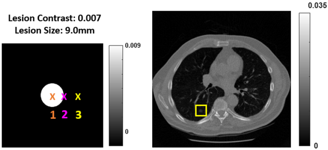
While the piecewise linear interpretation of neural networks is convenient, the question remains whether it is practical to analyse each linear region separately. In particular, deep networks tend to partition the input space into a large number of linear regions.7 It is also possible for networks to have unstable gradient - i.e., small perturbations in the inputs resulting in large changes in gradient or Jacobians. To investigate these behaviors for inputs relevant to CT denoising, we use example CT images as operating points and gradually insert perturbations of interest. For high dimensional input spaces in neural networks, there are many potential types of perturbations that may be explored. Here, we choose clinically relevant perturbations like lesion features of interest (e.g., contrast, shape, texture), noise, or background the lesion is embedded in. We record the activation pattern associated with each perturbation and report the number of changes in activation indicators from the operating point and the total number of activation patterns through the range of perturbations. Furthermore, we compare the Jacobians in neighboring linear regions. In this work, the operating point was chosen as a region of interest (ROI) containing a spherical, uniform lesion with diameter 9.0 mm and contrast 0.007 mm−1 in the lung region of thorax CT scan as shown in Fig 1. Results shown below pertain to lesion contrast from 0.007 to 0.04 mm−1 in small increments of 2 × 10⁻⁷ mm−1 .
Figure 1:

The operating point μo was chosen as a uniform spherical lesion in the lung region of a thorax CT scan. We present the local Jacobian for three locations at the center, edge, and background of the lesion.
2.3. Extent of approximately locally linear regions
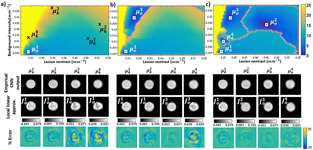
Through initial experimentation, we observed that the Jacobians for neighbouring linear regions are similar. We therefore investigate whether we can extend the boundary of locally linear regions to include multiple strictly linear regions with approximately the same Jacobian. Using the same operating point μo and perturbation scheme in the previous section, we compute the output of perturbed inputs μk using the Jacobians for μo (the right hand side of Eq. 5) and compare it with the true CNN output. For initial investigation in this work, we compare the maximum (over voxels) absolute percent error between the two and set a threshold below which the two outputs are considered similar enough and that the inputs fall within the same linear region. We developed strategies to choose different operating points so that the percentage error throughout the range of perturbations falls below the threshold. For results shown below, we present the linear regions and associated operating points for an input space encompassing two types of perturbations - lesion contrast ranging from 0.001 to 0.08 mm−1 and the intensity of a uniform background the lesion is embedded in from 0 to 0.04 mm−1.
2.4. Neural network analysis based on locally linear regions
Using the approximately linear regions identified above, we may apply linear system analysis tools to each linear region to understand and explain some of the overall nonlinear and data-dependent behaviors of neural network algorithms. To ensure generality without assumptions of shift-invariance, we performed SVD of the Jacobians for each approximately linear region. Then, by projecting inputs of interest μin onto the singular basis vectors, we can analyze which features of the inputs that are considered preserved, denoted as (i.e., with singular values above a certain threshold) and which features are attenuated, denoted as (i.e., with singular values below a certain threshold). Mathematically:
| (7) |
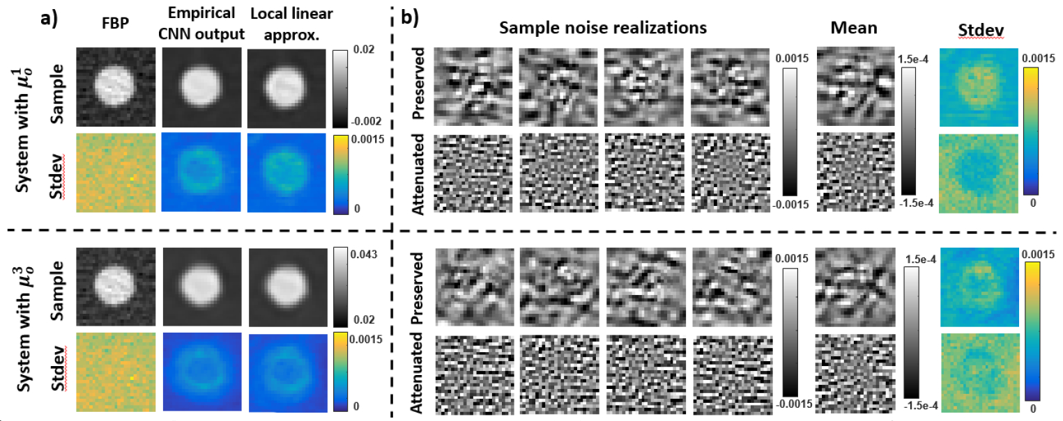
where si and vi are the ith singular value and basis vector, and ϵ is the threshold on singular values, chosen as 0.10 in this work. We applied the SVD analysis to noisy input images to visualize how the network “denoises”. In this case, the perturbation, μk – μo, is noise. We generated 100 different noise realizations at a noise level comparable to the training dataset, and decomposed each realization to the “preserved” and “attenuated” components according to Eq. 7. The mean and standard deviation over all noise realizations are presented to visualize how neural network reduces noise.
2.5. Experimental setup
In this work, we applied the above analysis to a network based on the REDCNN architecture.8 We identified 2900 slices from thorax CT scans in the LIDC database9 and use them as ground truth to generate the training data. The normal and low dose training pairs were generated from filtered-backprojection reconstruction using a barebeam fluence of I0 = 105 and I0 = 1.25 × 10⁴, respectively.
3. RESULTS
We first present results showing the extent of strictly linear regions as a function of lesion contrast from the operating point in Fig.1. Combining the number of cumulative activation patterns in Fig.2a and the number of indicator change in Fig.2b, we may infer how many strictly linear regions there are within the range of perturbations investigated. Zooming in on two small range of contrast in Fig.2c, both the cumulative number of activation patterns and the number of indicator changes have the same trend. The perturbation increment was chosen small enough that the input either stays in the same linear region, or transition to a neighboring linear region with at most one ReLU change. Note that while the cumulative activation patterns either stays the same or increases (by definition) for each contrast increment, the number of indicator change may also decrease. Overall, the neural network has seen 33992 strictly locally linear regions for the range of lesion contrast investigated. We further present a profile through the Jacobian matrix that passes through each of the three locations identified in Fig.1. The Jacobians are different from lesion center, to edge, to background, indicating a linear but shift-variant system. Comparing amongst the different strictly linear regions in each portion of the plot, the Jacobians are very similar despite belonging to different linear systems. Investigations into strictly locally linear regions reveal that the transition between neighboring linear region is sensitive to small changes in perturbations but the Jacobians are similar. We therefore investigate whether the input space can be partitioned into fewer approximately linear regions using methods in Sec.2.3. We perturbed both the lesion contrast and the lesion background intensity and plotted the maximum absolute percent error between local linear approximation and CNN output. Four example inputs at different contrast and background (labeled μk) are presented showing comparisons between the empirical CNN output, a linear approximation using Jacobians at an operating point (labeled μo), and the percentage error map between the two. Fig.3a shows the approximation errors for just one operating point shown in Fig.1. The error is 0 at the operating point and increases as we move further away. Fig.3b and 3c shows the approximations error improving as we use more operating points. Compared to 33992 strictly locally linear regions in just one dimension (Fig.2), the linear approximation method yields a much small number of linear systems that is practical to analyze. Using the approximate local regions identified in Fig.3c, we performed SVD analysis on two locally linear systems with operating points and . We chose inputs belonging to each linear region and added noise as perturbations. The inputs contains lesions of the contrast, noise magnitude, and noise correlation; the only difference is the background intensity. Fig.4a shows the FBP input, empirical CNN output, and its linear approximation for both a sample noise realization and standard deviation maps over 100 noise realizations. Good agreement was observed between the CNN outputs and linear approximations for the case, indicating that noise perturbations can be approximated by the same linear system at the operating point. The noise magnitude was well-approximated for the case but the spatial distribution could be improved, which suggests that the criteria for linear approximation should be revisited for noise prediction. Comparing the two linear regions, the one based on imparts greater noise reduction seen from the lower standard deviation magnitude. Fig.4b shows the “preserved” and “attenuated” input features (Eq.7) for four sample noise realizations as well as the mean and standard deviation maps over 100 noise realizations. The attenuated portion is high frequency and appears noise-like for both systems - consistent with the “denoising” purpose of the network. The preserved signal is smoother outside the lesion but contains more mid- to high-frequency variations inside the lesion. Both the preserved and attenuated signals are space-variant, with more noise removal in uniform regions (outside and inside the lesion) compared to the edges. This behavior is more obvious in the mean and standard deviation images.
Figure 2:

a) Number of cumulative activation pattern over the range of lesion contrast 0.007 ~ 0.04mm−1 b) Number of activation indicator change over the same range of lesion contrast c) Top row: Zoom-in view of the curve in b), which shows three strict linear regions and overlays their local Jacobians at three lesion locations. Bottom row: Similar contents for the other zoom-in region (lower lesion contrast)
Figure 3:

a) Top row: Map of maximum local linear approximation error with increasing lesion contrast and background intensity for system with operating point ; Bottom row: four lesion inputs of interest with increasing approximation error. b) Top row: Input space being partitioned by applying two operating points; Bottom row: lesion inputs of interest evaluated by two systems. c) Top row: Input space being partitioned by applying four operating points; Bottom row: lesion inputs of interest evaluated by each of the system
Figure 4:

a) Top row: Sample noisy realization and standard deviation map across 100 different realizations for noisy FBP input, CNN output and local linear approximation by using system with operating point ; Bottom row: Similar contents by using system with . b) Top row: Preserved and attenuated features from SVD analysis for sample noise realizations, mean and standard deviation maps across 100 noise realizations by using system with operating point ; Bottom row: Similar contents for system with
4. DISCUSSION AND CONCLUSION
In this work, we presented a method for analyzing piecewise linear neural networks. We observed rapid transitions between strict locally linear regions and introduced an approximation method to make the analysis more tractable. Linear system analysis tools such as the SVD were applied to explain some of the nonlinear and data-dependent behavior of an example denoising network, specifically, what input features can be preserved and which are not. The most significant challenge with this type of analysis is the high dimensional input space. We chose to use clinically relevant image features as “perturbations” or search directions to map out the locally linear regions. Future work will encompass a wider range of perturbations so that neural network performance can be analyzed in relation to whether image features important for diagnosis can be preserved. Furthermore, we will investigate strategies to identify maximally separated operating points in the input space such that the analysis remains tractable.
REFERENCES
- [1].Gang GJ, Guo X, and Stayman JW, “Performance analysis for nonlinear tomographic data processing.” SPIE-Intl Soc Optical Eng, 5 2019, p. 124. [DOI] [PMC free article] [PubMed] [Google Scholar]
- [2].Solomon J, Lyu P, Marin D, and Samei E, “Noise and spatial resolution properties of a commercially available deep learning-based ct reconstruction algorithm,” Medical Physics, vol. 47, pp. 3961–3971, 9 2020. [DOI] [PubMed] [Google Scholar]
- [3].KC P, Zeng R, Farhangi MM, and Myers KJ, “Deep neural networks-based denoising models for ct imaging and their efficacy.” SPIE-Intl Soc Optical Eng, 2 2021, p. 16. [Google Scholar]
- [4].Lee G-H, Alvarez-Melis D, and Jaakkola TS, “Towards robust, locally linear deep networks,” 7 2019. [Online]. Available: http://arxiv.org/abs/1907.03207 [Google Scholar]
- [5].Goodfellow IJ, Shlens J, and Szegedy C, “Explaining and harnessing adversarial examples,” 12 2014. [Online]. Available: http://arxiv.org/abs/1412.6572 [Google Scholar]
- [6].Raghu M, Poole B, Kleinberg J, Ganguli S, and Dickstein JS, “On the expressive power of deep neural networks,” 2017. [Google Scholar]
- [7].Montúfar G, Pascanu R, Cho K, and Bengio Y, “On the number of linear regions of deep neural networks,” 2 2014. [Online]. Available: http://arxiv.org/abs/1402.1869 [Google Scholar]
- [8].Chen H, Zhang Y, Kalra MK, Lin F, Chen Y, Liao P, Zhou J, and Wang G, “Low-dose ct with a residual encoder-decoder convolutional neural network,” IEEE Transactions on Medical Imaging, vol. 36, pp. 2524–2535, 12 2017. [DOI] [PMC free article] [PubMed] [Google Scholar]
- [9].Hancock MC and Magnan JF, “Lung nodule malignancy classification using only radiologist-quantified image features as inputs to statistical learning algorithms: probing the Lung Image Database Consortium dataset with two statistical learning methods,” Journal of Medical Imaging, vol. 3, no. 4, p. 044504, 2016. [DOI] [PMC free article] [PubMed] [Google Scholar]


