

Abstracts
Background
The aim of this study was to evaluate the most effective combination of autoregressive integrated moving average (ARIMA), a time series model, and association rule mining (ARM) techniques to identify meaningful prognostic factors and predict the number of cases for efficient COVID-19 crisis management.
Methods
The 3685 COVID-19 patients admitted at Thailand’s first university field hospital following the four waves of infections from March 2020 to August 2021 were analyzed using the autoregressive integrated moving average (ARIMA), its derivative to exogenous variables (ARIMAX), and association rule mining (ARM).
Results
The ARIMA (2, 2, 2) model with an optimized parameter set predicted the number of the COVID-19 cases admitted at the hospital with acceptable error scores (R2 = 0.5695, RMSE = 29.7605, MAE = 27.5102). Key features from ARM (symptoms, age, and underlying diseases) were selected to build an ARIMAX (1, 1, 1) model, which yielded better performance in predicting the number of admitted cases (R2 = 0.5695, RMSE = 27.7508, MAE = 23.4642). The association analysis revealed that hospital stays of more than 14 days were related to the healthcare worker patients and the patients presented with underlying diseases. The worsening cases that required referral to the hospital ward were associated with the patients admitted with symptoms, pregnancy, metabolic syndrome, and age greater than 65 years old.
Conclusions
This study demonstrated that the ARIMAX model has the potential to predict the number of COVID-19 cases by incorporating the most associated prognostic factors identified by ARM technique to the ARIMA model, which could be used for preparation and optimal management of hospital resources during pandemics.
Keywords: COVID 19, Pandemic, Data mining, Time series analysis, Association rule mining
Background
The crisis outbreak of coronavirus disease 2019 (COVID-19) caused by severe acute respiratory syndrome coronavirus 2 (SARS-CoV-2) started in Wuhan, Hubei Province, China in December 2019 [1]. The COVID-19 pandemic has required governments around the world to implement new policies under pressure from vulnerable people and communities [2]. Since the first outbreak, COVID-19 has mutated into many variants including the alpha, beta and delta SARS-COV-2 variants, which have been associated with new waves of infection [3]. The catastrophic effect across the entire world resulted in more than six million deaths worldwide in 2022 [4]. In addition, COVID-19 has caused a rapid deterioration in the condition of the disease, and the number of patients requiring hospitalization has increased significantly, resulting in a high demand for hospital resources [1].
Data mining is an efficient analytical methodology to recognize and investigate a huge data set to acquire meaningful information [5]. In the medical field, the large numbers of medical records (including demographic information, diagnoses, clinical notes, etc.) in the healthcare information systems are ideal targets for the use of data mining in improving the analysis and prognosis prediction of various diseases [6–8]. Examples include using an Artificial Neural Network (ANN) and Support Vector Machine (SVM) algorithm to predict cardiovascular disease [9], using data mining classification algorithms, Decision Tree and Naive Bayes algorithms to identify liver disease [10] and predict the recovery outcome of Middle East Respiratory Syndrome Coronavirus (MERS-CoV) [11]. With the unprecedented increase in COVID-19 cases worldwide, there is a need for effective prediction models to identify the associated prognostic factors and forecast the number of COVID-19 cases to optimally organize the hospital resources.
Time series analysis and association rule mining (ARM) models have been widely used to predict trends, structural breaks, cycles, and unobserved values, and have proven to be useful in the medical field [12–14]. The auto regressive integrated moving average (ARIMA), a time series analysis model, was shown to have a promising accuracy for forecasting of infectious diseases in medical fields [15, 16]. ARIMA was used to forecast the number of new COVID-19 cases, deaths, and recoveries based on the daily reported data from different countries for assessment of the future outbreak [17–20]. ARM was originally presented by Agrawal et al. as an algorithm for marketing data analysis [21]. ARM has been used to extract medical health information, which is currently being applied for the development of classification and prediction models to identify and forecast the possibility of development and progression of a disease by considering the rules of the disease [22]. ARM was demonstrated to be an effective model for mining the frequent symptom pattern for COVID-19 patients, which could assist clinicians in decision making [23]. Another study used ARM to analyze the patterns of different non-pharmaceutical interventions to manage the infection growth rate in the United States [24]. Even though there are many advanced data-driven time series methods used to predict the future number of COVID-19 patients, a new and more accurate prediction model is important in the pandemic crisis. The associated contributing factors should be considered to improve model performance. Therefore, the combination of ARM and ARIMA models by selecting the most associated prognostic rules and integrating with ARIMA models could increase the accuracy of predicting new cases to better understand the current situation and the progression of COVID-19, which can be easily used by society, organizations, or governments to assess and manage the crisis during the future outbreak.
The aim of this study was to evaluate the most effective combination of ARM techniques and ARIMA models to identify prognostic factors and predict the number of COVID-19 patients. These models are expected to allow for better preparation, organizing hospital resources of further such units and more optimal use of medical personnel and equipment to enhance healthcare decision-making to manage COVID-19 patients in this crisis situation.
Methods
Administration protocol and data collection
The study was conducted at Thailand’s first university-based field hospital. The field hospital was transformed from the service apartment style 14-story building of the university dormitory into a 494-bed facility for non-critical COVID-19 patients [25]. The field hospital was managed by the main university hospital and included the patients referred from the project’s five university hospitals and hospitals in the central area of Thailand. Sources of funding come mainly from the donations of university alumni, community groups and non-governmental organizations. Upon admission, a nurse records patient data in the COVID-19 screening of the field hospital information system; the patient undergoes a chest x-ray, blood tests for complete blood count (CBC), liver function tests (LFTs), electrolyte, balance urine nitrogen (BUN), and Creatinine (Cr). The doctor interprets the labs and chest x-ray, and records the results in the admission note. The patients are only admitted to the field hospital if they meet all of the following criteria: 1) asymptomatic, mild or moderate symptoms; 2) normal activities of daily living; 3) no important organ dysfunction; 4) no psychiatric history; and 5) resting pulse oxygen saturation (SpO2) > 95%. To avoid unnecessary contact between patients and medical personnel, the patient reports signs and symptoms, wants and needs via an internal field hospital application. Any consultation with the attending physician is done through a notification form. If the attending physician wishes to speak to the patient, the patient’s telephone number is obtained from the respective patient’s floor. All prescriptions must be made using a prescription form which will then be processed by the attending nurse and recorded in the progress note in the field hospital information system and in the university hospital electronic medical record system. In this field hospital system, the laboratory and radiographic examination would be performed on symptomatic COVID-19 patients with a history of taking Favipiravir and for severity assessment of symptomatic COVID-19 patients.
For Favipiravir-naive patients: 1) A follow-up chest x-ray may be considered in patients with worsening signs and symptoms (body temperature (BT) > 38.0 °C, cough, fatigue, SpO2 < 96%, or decreased SpO2 > 3% after a stress test); and 2) if the chest x-ray infers pneumonia with respiratory signs and symptoms (as mentioned in 1), refer the patient to the originating hospital for continued treatment with Favipiravir.
For patients previously treated with Favipiravir: 1) Follow-up by chest x-ray, LFTs); 2) if LFTs increase, consider consulting an ID specialist to terminate/adjust medication use; and 3) if the chest x-ray infers a progression of the infiltration accompanied by respiratory signs and symptoms (cough, fatigue, SpO2 < 96% and SpO2 drop > 3% after a stress test), consider referring the patient to the hospital of origin.
Asymptomatic patients who have been hospitalized for at least 14 days after a positive COVID-19 testing will be discharged home. The patients who received Favipiravir should fulfil all the following criteria: 1) The patients signs and symptoms have improved without progression of infiltration on chest x-ray; 2) BT < 37.8 °C continuously for 24–48 hours; 3) respiratory rate (RR) < 20/min; and SpO2 > 96% at rest. In the event of a patient’s condition deteriorating, they are quickly transferred to the designated higher-level hospitals.
The criteria for transfer are 1) meeting the criterion of severe or critical, and 2) lung imaging showing a greater than 50% progression of lesions. Patients do not need Real-time Polymerase Chain Reaction (RT-PCR) or Antigen/Antibody detection for COVID-19 prior to discharge. One day before discharge, the attending nurse informs the attending physician of the number of potential discharges, so that the physician can prepare medical certificates and insurance documents according to the patient’s needs. Upon discharge, the attending physician updates the patient’s progress and discharge summary in the electronic medical record system of the university hospital.
A total number of 3685 patient records were retrieved from the electronic hospital information systems of the referral hospitals and the field hospital information system. In this study, we included all patients confirmed with asymptomatic and mild-to-moderate COVID-19 conditions from March 2020 to August 2021 (four waves of COVID-19 in Thailand). Collected data included patient demographics, comorbidities, body mass index (BMI), job, place of exposure to coronavirus, symptom before field hospital admission, sign of pneumonia in chest x-ray, field hospital length of stay, and the field hospital discharge destination. Table 1 shows the preliminary analysis of the dataset, including attributes, values, and frequency of each attribute-value pair.
Table 1.
Preliminary analysis of the dataset: attributes, values, and frequency of each attribute-value pair
| No | Attribute name | Attribute value | Attribute code | Frequency |
|---|---|---|---|---|
| 1 | Gender | Male | sex_male | 1711 |
| Female | sex_female | 1974 | ||
| 2 | Age (year) | Less than 24 | age_24 | 1148 |
| 25–44 | age_45_44 | 1838 | ||
| 45–64 | age_45_64 | 625 | ||
| More than 65 | age_65 | 74 | ||
| 3 | Body Mass Index | Less than 25 | bmi_25 | 2309 |
| 25–29 | bmi_25_29 | 931 | ||
| More than 30 | bmi_30 | 445 | ||
| 4 | Underlying | None | ud_none | 3392 |
| Diseases | Respiratory | ud_repp | 82 | |
| Hypertension | ud_ht | 39 | ||
| Metabolic | ud_meta | 53 | ||
| Dyslipidemia | ud_dlp | 14 | ||
| Other | ud_oth | 64 | ||
| Diabetes mellitus | ud_dm | 18 | ||
| Pregnant | ud_preg | 23 | ||
| 5 | Job | General worker | job_gen | 3592 |
| Healthcare worker | job_health | 93 | ||
| 6 | Source of infection | Community | source_com | 3119 |
| Family | source_fam | 475 | ||
| Hospital | source_hosp | 91 | ||
| 7 | Symptom | Asymptomatic | symp_ast | 2295 |
| Mild | sym_mild | 1371 | ||
| Moderate | sym_mode | 19 | ||
| 8 | Chest X-ray | No lesion | cxr_no | 3213 |
| Pneumonia | cxr_pneu | 472 | ||
| 7 | Length of stay (Day) | Less than 14 | los_1_14 | 3625 |
| More than 14 | los_15 | 60 | ||
| 8 | Patient Discharge | Home discharge | dc_home | 3600 |
| Refer to general hospital | dc_hosp | 85 | ||
| 9 | Current Incidence | Wave 1 (MAR-MAY 2020) | wave_1 | 55 |
| Wave 2 (JAN-MAR 2021) | wave_2 | 311 | ||
| Wave 3 (APR-MAY 2021) | wave_3 | 1779 | ||
| Wave 4 (JUN-JUL 2021) | wave_4 | 1540 |
Time-series analysis and association analysis
In this work, we present a study to combine time series analysis and association analysis to forecast the COVID-19 admitted cases as well as to analyze their potential factors and characteristics. To estimate the number of new cases and to predict the prognosis for better understanding of the current situation and progression of COVID-19, we exploited the autoregressive integrated moving average (ARIMA) model and its subclasses (i.e., AR, MA, ARMA) [12, 17, 26], and association rule mining (ARM) [21, 24] as tools for investigation (Fig. 1).
Fig. 1.

The summary of the time series and association analysis
The autoregressive (AR) model
In the AR model, the predictive value at the time period t is modeled by the observed values at various time slots t − 1, t − 2,. . ., t − k. The impact of the value at each previous time period on the value at the current time is determined by the coefficient factor at that particular period of time. With this assumption, the model performs the regression of past time series and then calculates the present or future values in the series, commonly known as an auto regression (AR) model. It can be modeled as follows.
Here, yt is the value at the current time t, and yt − 1, yt − 2, …, yt − p are the observed values at the previous p time spots with their corresponding coefficients β1, β2, …, βp, respectively, β0 is the intercept, and εt is the residual error at the time t. Therefore, yt − εt is the expected value at the current time t. In this work, the value yt can be modeled as the number of inpatients, incoming patients, or outgoing patients at the time period t.
The moving-average (MA) model
Since the value of the time period t may be impacted by unexpected external factors, i.e., noises, we can alleviate such impact by means of the moving average method. Analogous to AR, the predicted value at the time period t can be modeled by the previous q lagged forecast errors ϵi as follows.
Here, yt is the value at the current time t and the lagged errors εt − 1, εt − 2, …, εt − q are residual errors of the q autoregressive models at time t − 1 to t − q with ϕ1, ϕ2, …, ϕq as their corresponding coefficients, ϕ0 is the intercept, and yt is the residual error at the time t. The residual error at the time points after t − 1 can be derived by the auto-regressive (AR) model as follows.
Although the standard AR and MA may use the auto-correlation function (ACF), which takes into account all of the points, it is possible to apply the partial auto-correlation function (PACF), which accounts for the values of the intervals between.
The autoregressive moving average (ARMA) model
The Auto Regressive Moving Average Model (ARMA) combines the AR and MA models. In ARMA, the impact of previous lags along with the residuals is considered for forecasting the future values of the time series as follows.
Here, βi represents the coefficients of the AR model, ϕi represents the coefficients of the MA model, and εt is the residual error at the time t. We assume only one significant value from the AR model and one significant value from the MA model, so the ARMA model will be obtained from the combined values of these two models, denoted as the order of ARMA (1,1).
The autoregressive integrated moving average (ARIMA) model
As a generalization of AR, MA, and ARMA, the ARIMA model introduced differencing (integration) into the ARMA model to make the series stationary exploit to forecast future values under the factor of previous lag value and residuals errors. Besides manipulating the time lag and alleviating noise by smoothing, it is also possible to decompose a series into trend, seasonal, and residual components, by assuming an additive model. With this addition, the series can be transformed to a stationary time series. To achieve the transformation, the differencing method is applied. For example, we can subtract the t − 1 value from t values of time series. After applying the first differentiation, if we are still unable to get the stationary time series, we can again apply the second-order differentiation. The ARIMA model is an extension of the ARMA model by the fact that it includes one more factor known as integrated (i.e., differentiation) which stands for I in the ARIMA model. The ARIMA model, denoted by ARIMA (p,d,q), can be formulated as follows:
Here, p is the order of the autoregressive process, d (set to 1 in this case) is the degree of differentiation (the number of times the series was differenced), and q is the order of the moving average component. In this model, the first-order difference (d = 1) between consecutive observations y′i was computed and used, instead of the original observed value yi as shown below.
Differencing removes the changes in the level of a time series, eliminating trend and seasonality and, consequently, stabilizing the mean of the time series.
In some situations, we may need to difference the series data a second time (d = 2) to obtain a stationary time series, which is referred to as second order differencing as follows:
A higher-order differentiation can be pursued analogously in the same manner.
The autoregressive integrated moving average with exogenous covariates (ARIMAX) model
When an ARIMA model includes other time series as input variables, the model is referred to as an Autoregressive Integrated Moving Average with Exogenous Covariates (ARIMAX) model. An ARIMAX model can be viewed as a multiple regression model that takes the impact of covariates on the forecasting into account, improving the comprehensiveness and accuracy of the prediction. The ARIMAX(p,d,q) extends the ARIMA(p,d,q) model by including the linear effect that one or more exogenous series has on the stationary response series yt. This method is suitable for forecasting when data is stationary/non-stationary, and multi-variate with any type of data pattern, i.e., level/trend/seasonality/cyclicity. The ARIMAX(p,d,q) model can be formulated as follows:
Here, d is set to 1, (Xi)t is the value at the time t of the i - th exogenous covariable (X1), θi is the corresponding coefficient for the covariable Xi, and m is the number of exogenous covariables to be considered, while p, d, and q indicate the same parameters as in the ARIMA model.
Association rule mining
Besides the time-series analysis, association rule mining (ARM) can be used as a multivariate analysis to help us understand the correlation among factors [24]. Given a dataset containing a collection of records or transactions, each record comprises a set of categorical attributes. An association rule can be denoted by A → B, where A (the antecedent or LHS) and B (the consequent or RHS) are sets of various attribute-value pairs (also called itemsets), and are disjoint. The rule represents the hypothesis that when variables in A occur in the dataset, the variables in B also occur. Association mining generates a large number of rules from a given dataset. In a dataset with m attributes n − 1 antecedents and one consequent, each with n values, each can generate a maximum of nmn − 1 − 1 rules. However, not all rules are significant. The goal of this approach is to find rules that have high practical significance. To eliminate spurious rules, we use three measures: support, confidence, and lift. In addition, we also use the chi-squared test to measure the statistical significance of the association between the antecedent and the consequent. Given two disjoint sets of attribute-value pairs A and B, and an association rule A → B; support of the rule refers to the number of records where the attribute-value pairs in either set A or B appear in the dataset relative to the total number of records (transactions or instances). This denotes the prevalence of the rule in the dataset. By definition, the support value is symmetric, that is Support (A → B) = Support (B → A), and it equals the total numbers of records containing both A and B to the total number of records in the dataset. The confidence of the rule A → B measures the conditional probability of B, given A. Thus, the confidence measure for a given rule is asymmetric, that is Confidence (A → B) ≠ Confidence (B → A). The lift measure is the ratio between the observed support and the expected support between the independent variables A and B. Implicitly, lift > 1 means a greater degree of dependence, lift < 1 specifies negative dependence, and lift = 1 indicates independence between A and B. Lift is also a symmetric measure between the itemsets A and B, that is Lift (A → B) = Lift (B → A).
Here, |A| and |B| are the numbers of records that include A and B, respectively, while ∣A ⋂ B∣ is the number of records that contain both A and B. In this paper, the antecedent A can be either patient demo-graphics (either male or female), age (< 24, 25–44, 45–64, and > 65), body mass index or BMI (< 25, 25–29, and > 29), underlying diseases (none, respiratory, hypertension, metabolic, dyslipidemia, diabetes mellitus, pregnant, or others), job (healthcare or non-healthcare patient), inflection source (community inflection, family inflection, or hospital inflection), symptoms before field hospital admission (asymptomatic, mild, or moderate), sign of pneumonia in chest x-ray (no lesion or pneumonia) or length of stay in the field hospital (14 or > 14), and patient discharge (home discharge or refer to general hospital), as the contributing factors. On the other hand, for the consequent B we focus on (1) the length of stay (either 1–14 or > 14), (2) the patient discharge (either home discharge or hospital discharge), (3) the chest x-ray result, and (4) current incidence (wave 1, 2, 3 or 4). Since one assumption for ARM is that all the values of attributes are discrete, we translate the numerical data used in the study into discrete labels, as well as split the continuous data of infection growth curve into four phases.
Experiment settings
Data collection and parameter settings
The dataset includes 3685 records registered with the electronic hospital information systems of the field hospital during March 2020 to August 2021. It displays characteristics of the dataset, including, attributes, values, and frequency of each attribute-value pair. Each of the nine attributes contains 2–8 possible values. Most attributes have imbalanced numbers in their values, except gender (Table 1). In our time series analysis, the target of prediction is the number of patients in the field hospital for each day during the observation period, that is March 2020 to August 2021. We have explored the value of the three ARIMA parameters as p ∈ {1, 2, 3}, d ∈ {1, 2}12, q ∈ {1, 2, 3} due to our preliminary test. In addition, we applied association rule mining to find the most influential factors among the eleven factors, that is patient demographics, age, body mass index, underlying diseases, job, inflection source, symptom before field hospital admission, sign of pneumonia in chest x-ray, length of stay in the field hospital, patient discharge, and current incidence. As an ARIMAX model, we extend the ARIMA(p,d,q) model to include the parameters as a series that are the most influential to the prediction of the number of patients in the hospital. The parameters included are known as exogenous series that are expected to trigger the stationary response on the series that we are predicting.
Performance metrics and evaluation
Given a data set has n values, denoted by y1,. .., yn, each associated with a predicted value f1,. .., fn, the following three metrics can be formulated. Coefficient of determination (R2) is the proportion of the variation in the dependent variable that is predictable from the independent variable(s) as follows:
| 1 |
| 2 |
| 3 |
| 4 |
Here, SSr is the sum of squares of residuals, SSt is the total sum of squares, proportional to the variance of the data, and is the mean of the observed data. Ranging from 0 to 1, it provides a measure of how well observed outcomes are replicated by the model. The higher the coefficient value is, the closer the dependent variable and independent variable are.
Root mean square error (RMSE) the standard deviation of the prediction errors [27], which are a measure of the distance of the data from the regression line, indicating the concentration of the data around the line of best fit as follows:
| 5 |
It expresses the dispersion of these errors.
Mean absolute error (MAE) allows measurement of the average magnitude of the errors for a set of predictions, regardless of their direction.
| 6 |
It represents the mean of the absolute difference in the sample between the prediction and the actual observation, taking into account that all individual differences are of equal significance. Therefore, compared to RMSE, MAE is less sensitive to outliers.
Results
Time series analysis
This section presents a time series analysis to forecast the number of patients admitted to the field hospital. Figure 2 shows the number of patients from 26 March 2020 to 22 July 2020. Three time series represent the relationships among a number of residing patients that are equal to a cumulative difference between admitted and discharged patients living in the hospital. The graph presents four waves of pandemic following the number of patients in hospital. The four waves are as follows: The first wave (Wave 1), the emergence of SAR-CoV-2, is the smallest period (34 days) from 26 March 2020 to 16 May 2020. The second wave (Wave 2) was from 11 January 2021 to 14 March 2020 (44 days). After that, the third wave (Wave 3) and fourth wave (Wave 4) were the continuous periods from 11 April 2021 to 31 May 2021 (51 days) and 1 June 2021 to 22 July 2021 (52 days), respectively. Finally, the forecasting models are validated by a test dataset from 1 August 2021 to 30 August 2021(30 days).
Fig. 2.

The number of daily data of patients in the field hospital; New patients; Admitted Patients; Discharged Patients in four waves of COVID-19 pandemics in Thailand
In this study, the time series models were trained using six training datasets. The first training set (All Wave) covers all datasets Wave 1 to Wave 4 of 228 days; the second training set, Wave 1 of 34 days; the third training set, Wave 2 of 45 days; the fourth training set, Wave 3 of 51 days; the fifth training set, Wave 4 of 52 days; the sixth training set, Wave 3 and Wave 4 of 103 days.
In this work, we tested the estimated model using an autocorrelation function (ACF) and a partial autocorrelation function (PACF) plots to ensure that the model fits the data [17]. Figure 3 presents the steady-state prediction of time-series models. An estimation of the model explored the coefficient (Coef.), the standard error (Std err.) and z. An estimate of the first model was the AR model which gave a coefficiency of 0.3808, standard error of 0.243 and z of 1.565. The second model was an MA model which gave coefficiency of − 0.5287, standard error of 6.841 and z of − 0.077. The sigma value or constant value was coefficiency of − 0.5287, standard error of 6.841 and z of − 0.077. Moreover, we further estimated the model with Jarque-Bera of 7.70, heteroskedasticity of 0.57 and skew of 0.68.
Fig. 3.

An autocorrelation function (ACF) and a partial autocorrelation function (PACF) are presented to confirm the steady-state prediction of time-series models
For the data set, the time series method was applied using Python (PyFlux library) for time series analysis and prediction to compare the criteria of each setting. The ARIMAX (p,d,q) + X models were parameterized with X ∈ {ϕ, x1, x2}, p ∈ {0, 1, 2, 3}, q ∈ {0, 1, 2, 3}, d ∈ {0, 1, 2}, where X is additional exogenous variables, with 51 combinations. Moreover, we select key features from association rule mining such as symptoms, age, and underlying diseases, etc. X = ϕ specifies no additional exogenous variable used. X = x1 indicates additional exogenous variables. There are 15 variables, composed of three attributes in the symptom feature, four attributes in the age feature, and eight attributes in the underlying diseases feature. X = x2 represents four variables of the selected attributes, that is the ‘moderate’ symptom, the ‘more-than-65’ age, and the underlying diseases of ‘diabetes mellitus’ and ‘pregnant.’
The forecasting-accuracy metrics of the 51 models summarized on the six datasets and the evaluation of models with the measures of RMSE and MAE are shown in Table 2. The forecasts for the admitted patients with prediction confidential intervals (CI) between 5 and 95% are presented in Fig. 4 for ARIMA (2,2,2) and Fig. 5 for ARIMAX (1,1,1)+ x2. Overall, the most accurate estimation was obtained by improving from ARIMA (2, 2, 2) to ARIMAX (1, 1, 1) + x2 for the training set in Wave 4, covering from 11 April 2021 to 31 May 2021. For the first setting (All-Wave), the best model is ARIMA (1,2,1) with the RMSE of 22.8141 and MAE of 19.4133, which was closer to the actual data. For Wave-1, ARIMAX (2,2,2) + x2 performs the best with the RMSE of 277.9974 and MAE of 273.4644, which was the highest to the actual data of all models. For Wave-2, AR(1) + X1 model is the best with the smallest RMSE and MAE. Based on RMSE and MAE, the value of ARIMA (1,1,1) + X1 was the closest to the actual data in Wave-3. The RMSE and MAE of ARIMAX (1,1,1)+ X2 appeared to be the best predictive models.
Table 2.
The results of time series analysis model applied to six training sets obtained from statistical tests: Coefficient of determination (R2), Root mean square error (RMSE), Mean absolute error (MAE)
| No | Model | All Wave | Wave 1 | Wave 2 | Wave 3 | Wave 4 | Wave 3–4 | ||||||||||||
|---|---|---|---|---|---|---|---|---|---|---|---|---|---|---|---|---|---|---|---|
| R2 | RMSE | MAE | R2 | RMSE | MAE | R2 | RMSE | MAE | R2 | RMSE | MAE | R2 | RMSE | MAE | R2 | RMSE | MAE | ||
| 1 | I(1) | 0.0899 | 290.7718 | 283.8123 | 0.0331 | 325.9969 | 323.9485 | 0.0904 | 277.9974 | 273.4644 | 0.0328 | 94.5392 | 75.6991 | 0.0145 | 65.7031 | 65.7790 | 0.0522 | 63.3078 | 63.8452 |
| 2 | I(2) | 0.2199 | 188.6716 | 178.0013 | 0.2199 | 325.9572 | 323.9855 | 0.2972 | 285.9000 | 280.6391 | 0.0425 | 77.1222 | 68.0936 | 0.0048 | 83.1201 | 73.3845 | 0.0425 | 80.7247 | 71.4506 |
| 3 | AR(1) | 0.5835 | 52.9774 | 44.8681 | 0.5172 | 334.5952 | 332.3318 | 0.5186 | 318.9675 | 315.8692 | 0.2275 | 85.0022 | 67.6283 | 0.5543 | 60.0630 | 49.5482 | 0.4259 | 30.1341 | 25.6407 |
| 4 | AR(2) | 0.5326 | 48.9132 | 45.3217 | 0.5543 | 338.2526 | 336.1396 | 0.0169 | 298.2876 | 295.3547 | 0.0001 | 78.0756 | 66.2715 | 0.3493 | 35.2782 | 26.6954 | 0.1111 | 57.0969 | 46.8206 |
| 5 | AR(3) | 0.5026 | 71.3773 | 67.2935 | 0.5969 | 337.3307 | 335.1067 | 0.1671 | 292.9912 | 290.9822 | 0.0084 | 82.1250 | 69.8914 | 0.1274 | 53.4205 | 42.5510 | 0.1001 | 61.1195 | 51.1240 |
| 6 | MA(1) | 0.0004 | 176.9638 | 171.7192 | 0.0004 | 327.4278 | 325.3349 | 0.0004 | 294.4148 | 292.0716 | 0.0004 | 81.4992 | 72.4591 | 0.0004 | 81.6120 | 71.7955 | 0.0004 | 270.0047 | 265.8700 |
| 7 | MA(2) | 0.0003 | 205.0899 | 199.6313 | 0.0003 | 329.3588 | 327.2778 | 0.0004 | 328.9829 | 326.8977 | 0.0003 | 93.4902 | 85.6784 | 0.0003 | 148.8627 | 141.7412 | 0.0003 | 92.1310 | 83.2050 |
| 8 | MA(3) | 0.0001 | 307.5673 | 298.8213 | 0.0002 | 328.1374 | 326.0477 | 0.0000 | 333.1808 | 331.1216 | 0.0004 | 149.7222 | 145.0442 | 0.0001 | 125.3216 | 117.2491 | 0.0000 | 79.3442 | 68.9794 |
| 9 | ARMA(1,1) | 0.5741 | 40.8981 | 36.6221 | 0.5020 | 334.0945 | 331.8095 | 0.4767 | 315.0413 | 311.7129 | 0.1788 | 85.6014 | 69.1618 | 0.5161 | 42.8637 | 38.1547 | 0.3543 | 33.6863 | 26.0659 |
| 10 | ARMA(2,2) | 0.5062 | 67.3449 | 63.3953 | 0.6258 | 339.1666 | 337.0229 | 0.0006 | 299.0722 | 296.2244 | 0.5596 | 203.8326 | 202.3505 | 0.1104 | 56.4891 | 45.8304 | 0.0368 | 72.2012 | 61.3681 |
| 11 | ARMA(3,3) | 0.5089 | 68.0282 | 64.0255 | 0.6393 | 334.7573 | 332.3653 | 0.0009 | 306.0231 | 303.3267 | 0.1338 | 147.5160 | 142.7802 | 0.1028 | 56.5914 | 45.7511 | 0.3217 | 62.0183 | 56.2090 |
| 12 | ARIMA(1,1,1) | 0.4182 | 121.1567 | 105.5253 | 0.0007 | 327.7731 | 325.6391 | 0.3813 | 275.0749 | 269.6568 | 0.2256 | 61.1524 | 51.7814 | 0.5694 | 43.9619 | 38.7228 | 0.7279 | 35.4740 | 29.4524 |
| 13 | ARIMA(2,1,2) | 0.4496 | 188.1384 | 175.6110 | 0.1136 | 331.8481 | 329.6721 | 0.0337 | 274.7054 | 269.5087 | 0.5424 | 241.8948 | 239.8888 | 0.0361 | 60.5829 | 48.7030 | 0.8066 | 37.8168 | 33.3437 |
| 14 | ARIMA(3,1,3) | 0.5746 | 100.8429 | 93.3260 | 0.0072 | 327.6217 | 325.5377 | 0.1379 | 291.6125 | 282.3766 | 0.0935 | 145.4436 | 140.7227 | 0.0324 | 60.5233 | 48.3732 | 0.2291 | 99.0573 | 92.0246 |
| 15 | ARIMA(1,2,1) | 0.6227 | 22.8141 | 19.4113 | 0.0022 | 327.9731 | 325.8776 | 0.5564 | 307.1235 | 303.0277 | 0.1896 | 85.9017 | 69.5801 | 0.5616 | 43.7555 | 38.6440 | 0.3546 | 33.6537 | 26.0567 |
| 16 | ARIMA(2,2,2) | 0.5811 | 108.9374 | 99.9407 | 0.0042 | 330.6365 | 328.5217 | 0.0735 | 280.7723 | 274.8963 | 0.5010 | 221.8999 | 220.2538 | a0.5853 | a29.7605 | a27.6102 | 0.0367 | 78.2477 | 67.6000 |
| 17 | ARIMA(3,2,3) | 0.5684 | 105.7827 | 98.0635 | 0.0399 | 328.8342 | 326.6476 | 0.0782 | 269.6121 | 246.3643 | 0.7882 | 147.4570 | 143.0789 | 0.1616 | 85.7303 | 66.8601 | 0.3501 | 81.0317 | 75.6607 |
| 18 | I(1) + X1 | 0.0037 | 288.6017 | 283.7774 | 0.0490 | 326.2426 | 324.0655 | 0.0342 | 282.0157 | 279.3011 | 0.0000 | 99.6746 | 75.6989 | 0.0000 | 81.8578 | 72.0013 | 0.0044 | 103.9072 | 83.0929 |
| 19 | I(2) + X1 | 0.2592 | 212.5173 | 197.9378 | 0.2592 | 326.2460 | 324.1258 | 0.0005 | 286.8855 | 283.5395 | 0.0019 | 99.7003 | 76.0409 | 0.0048 | 83.1201 | 73.3845 | 0.0068 | 103.7216 | 83.5353 |
| 20 | AR(1) + X1 | 0.6067 | 610.2414 | 519.6976 | 0.1226 | 326.8148 | 324.8728 | 0.2344 | 232.7690 | 219.5232 | 0.4300 | 38.4820 | 32.1837 | 0.6319 | 249.6770 | 198.6695 | 0.0122 | 268.9514 | 263.4326 |
| 21 | AR(2) + X1 | 0.5362 | 67.2016 | 59.9040 | 0.1071 | 327.5698 | 325.6145 | 0.0035 | 263.3728 | 258.8025 | 0.6491 | 36.7028 | 29.6225 | 0.3990 | 88.3833 | 67.2515 | 0.8336 | 100.1792 | 83.2140 |
| 22 | AR(3) + X1 | 0.6796 | 75.6844 | 55.5952 | 0.0890 | 326.4052 | 324.4467 | 0.0017 | 271.8932 | 267.0636 | 0.6816 | 37.0752 | 29.5750 | 0.0373 | 59.1096 | 47.5392 | 0.8428 | 97.1527 | 78.2065 |
| 23 | MA(1) + X1 | 0.0001 | 252.3404 | 248.6892 | 0.1281 | 336.3468 | 334.3429 | 0.0013 | 298.9810 | 296.1156 | 0.0084 | 104.0982 | 76.0860 | 0.0313 | 87.0295 | 76.0244 | 0.0176 | 103.1149 | 81.7565 |
| 24 | MA(2) + X1 | 0.0702 | 221.6587 | 216.9112 | 0.2267 | 335.3732 | 333.4037 | 0.1160 | 336.7430 | 334.5787 | 0.0004 | 75.8666 | 55.0494 | 0.0382 | 134.9549 | 127.8984 | 0.0138 | 88.1465 | 75.0825 |
| 25 | MA(3) + X1 | 0.0005 | 317.8255 | 309.4642 | 0.1913 | 329.5174 | 327.5438 | 0.0001 | 334.6743 | 332.6033 | 0.0060 | 113.7286 | 77.5648 | 0.0139 | 118.1786 | 109.4121 | 0.0008 | 87.2773 | 72.8789 |
| 26 | ARMA(1,1) + X1 | 0.5916 | 413.4365 | 358.2175 | 0.1774 | 324.0025 | 322.1328 | 0.1541 | 251.9922 | 243.5882 | 0.4516 | 33.2501 | 26.5740 | 0.6405 | 220.4147 | 176.9939 | 0.6106 | 165.2220 | 163.3853 |
| 27 | ARMA(2,2) + X1 | 0.5949 | 424.4358 | 366.5745 | 0.0723 | 331.6259 | 329.4747 | 0.3369 | 399.6066 | 398.4546 | 0.7118 | 171.6618 | 170.5084 | 0.4607 | 160.5215 | 149.9203 | 0.4951 | 88.6736 | 83.4224 |
| 28 | ARMA(3,3) + X1 | 0.1833 | 113.5424 | 100.8362 | 0.2160 | 327.6383 | 325.7101 | 0.0107 | 339.7625 | 337.6229 | 0.5940 | 167.3714 | 164.8800 | 0.5863 | 107.5209 | 84.9299 | 0.0044 | 219.6314 | 192.1180 |
| 29 | ARIMAX(1,1,1) + X1 | 0.4182 | 183.8188 | 166.3895 | 0.1277 | 322.2422 | 320.3213 | 0.2574 | 267.9366 | 262.3262 | 0.5140 | 45.4581 | 37.5053 | 0.5694 | 43.9619 | 38.7228 | 0.7704 | 83.1827 | 79.9974 |
| 30 | ARIMAX(2,1,2) + X1 | 0.6784 | 124.4039 | 99.0967 | 0.2633 | 321.7203 | 319.9461 | 0.0425 | 285.4226 | 281.3559 | 0.6366 | 176.3529 | 174.5772 | 0.0361 | 60.5829 | 48.7030 | 0.8382 | 59.1795 | 47.6580 |
| 31 | ARIMAX(3,1,3) + X1 | 0.6510 | 149.8496 | 127.6797 | 0.0302 | 336.0062 | 333.9879 | 0.0007 | 253.1438 | 247.7629 | 0.1191 | 144.5963 | 139.6924 | 0.0324 | 60.5233 | 48.3732 | 0.3812 | 55.4460 | 50.4435 |
| 32 | ARIMAX(1,2,1) + X1 | 0.2403 | 143.0063 | 130.9023 | 0.1210 | 322.0322 | 320.1035 | 0.2928 | 278.2316 | 273.1433 | 0.4498 | 49.7481 | 41.2963 | 0.5616 | 43.7555 | 38.6440 | 0.7471 | 79.9917 | 76.4410 |
| 33 | ARIMAX(2,2,2) + X1 | 0.2168 | 95.7906 | 88.9073 | 0.3083 | 316.7929 | 315.1248 | 0.0490 | 287.2771 | 283.2256 | 0.5580 | 207.7418 | 206.2698 | 0.5853 | 29.7605 | 27.6102 | 0.1473 | 98.7315 | 80.6377 |
| 34 | ARIMAX(3,2,3) + X1 | 0.4787 | 63.5331 | 57.3825 | 0.1452 | 337.2546 | 335.2641 | 0.0016 | 257.9516 | 251.6657 | 0.0026 | 144.7672 | 139.9775 | 0.1616 | 85.7303 | 66.8601 | 0.4676 | 74.2653 | 70.1748 |
| 35 | I(1) + X2 | 0.0447 | 289.1389 | 281.2524 | 0.0041 | 326.0347 | 323.9383 | 0.0884 | 278.0144 | 273.4693 | 0.0000 | 99.6750 | 75.6992 | 0.0000 | 81.8175 | 71.9843 | 0.0044 | 103.9073 | 83.0939 |
| 36 | I(2) + X2 | 0.0105 | 249.4103 | 231.4904 | 0.0421 | 326.0106 | 323.9672 | 0.2082 | 284.7981 | 279.4427 | 0.0019 | 99.6955 | 76.0373 | 0.0048 | 83.2961 | 73.5082 | 0.0068 | 104.7077 | 83.9761 |
| 37 | AR(1) + X2 | 0.6156 | 255.7645 | 212.8672 | 0.5172 | 334.5952 | 332.3319 | 0.1727 | 302.2914 | 298.4389 | 0.0282 | 69.9752 | 58.5275 | 0.6311 | 249.1627 | 198.4651 | 0.5834 | 41.9315 | 35.5895 |
| 38 | AR(2) + X2 | 0.5858 | 64.0891 | 52.3809 | 0.5543 | 338.2531 | 336.1401 | 0.0007 | 293.3307 | 290.4134 | 0.0131 | 70.7792 | 58.5222 | 0.3373 | 82.2578 | 62.6506 | 0.4830 | 42.5877 | 37.2450 |
| 39 | AR(3) + X2 | 0.5264 | 28.4479 | 22.4192 | 0.5969 | 337.3308 | 335.1069 | 0.1030 | 298.6989 | 296.3389 | 0.0111 | 72.7548 | 60.1599 | 0.0092 | 57.7292 | 46.8582 | 0.4188 | 51.2708 | 45.6610 |
| 40 | MA(1) + X2 | 0.0004 | 191.3896 | 187.3443 | 0.0004 | 327.4278 | 325.3349 | 0.0064 | 303.3572 | 300.9790 | 0.0116 | 81.3063 | 71.5271 | 0.0307 | 98.0537 | 87.9097 | 0.1876 | 275.7095 | 268.5105 |
| 41 | MA(2) + X2 | 0.0003 | 208.8616 | 204.3860 | 0.0003 | 329.3588 | 327.2778 | 0.0071 | 329.9775 | 327.9153 | 0.0164 | 94.5079 | 86.0634 | 0.0638 | 143.4629 | 136.7615 | 0.0215 | 93.9181 | 84.8925 |
| 42 | MA(3) + X2 | 0.0000 | 313.7185 | 303.9636 | 0.0002 | 328.3339 | 326.2458 | 0.0050 | 333.2174 | 331.1693 | 0.0168 | 83.1832 | 74.0123 | 0.0624 | 136.5470 | 125.2288 | 0.0435 | 87.0651 | 77.3405 |
| 43 | ARMA(1,1) + X2 | 0.6070 | 188.6286 | 158.6611 | 0.5020 | 334.0945 | 331.8095 | 0.2345 | 301.7636 | 297.9054 | 0.0152 | 80.3589 | 66.8892 | 0.6260 | 208.8213 | 169.3105 | 0.6516 | 76.7976 | 69.1291 |
| 44 | ARMA(2,2) + X2 | 0.5069 | 71.3063 | 67.2141 | 0.6257 | 339.1664 | 337.0227 | 0.0149 | 301.8609 | 298.7972 | 0.5278 | 160.9546 | 157.4370 | 0.4919 | 188.1245 | 174.4431 | 0.3916 | 113.9236 | 106.8338 |
| 45 | ARMA(3,3) + X2 | 0.5675 | 30.4833 | 28.1090 | 0.1795 | 324.3882 | 322.5190 | 0.3004 | 308.7024 | 303.8821 | 0.5828 | 157.7017 | 154.2446 | 0.6386 | 253.0751 | 196.3018 | 0.1300 | 43.9619 | 38.7226 |
| 46 | ARIMAX(1,1,1) + X2 | 0.3531 | 168.2529 | 153.0882 | 0.0929 | 318.2668 | 316.3056 | 0.2369 | 268.3102 | 262.7485 | 0.4671 | 50.0191 | 41.8890 | a0.5695 | a27.7508 | a23.4642 | 0.7704 | 83.1909 | 80.0059 |
| 47 | ARIMAX(2,1,2) + X2 | 0.6484 | 174.1887 | 148.7599 | 0.2435 | 324.9496 | 322.5022 | 0.0147 | 269.1468 | 263.4866 | 0.6058 | 198.4915 | 197.1301 | 0.0519 | 59.5415 | 47.9796 | 0.8380 | 60.6156 | 48.6302 |
| 48 | ARIMAX(3,1,3) + X2 | 0.6375 | 170.1995 | 146.9692 | 0.1756 | 323.9133 | 322.0434 | 0.0324 | 275.3298 | 266.7312 | 0.0229 | 144.4264 | 139.5740 | 0.0474 | 59.5452 | 47.7400 | 0.0752 | 91.5523 | 75.5956 |
| 49 | ARIMAX(1,2,1) + X2 | 0.0823 | 124.5007 | 114.6162 | 0.1758 | 324.0920 | 322.2535 | 0.2380 | 277.5598 | 272.5563 | 0.4500 | 49.7456 | 41.2962 | 0.5460 | 43.4074 | 38.4491 | 0.7471 | 80.0006 | 76.4500 |
| 50 | ARIMAX(2,2,2) + X2 | 0.6342 | 40.4552 | 34.6242 | 0.0904 | 277.9974 | 273.4644 | 0.0191 | 270.5990 | 264.7709 | 0.5524 | 217.1144 | 215.5897 | 0.0927 | 85.8890 | 67.4658 | 0.8189 | 72.6105 | 57.7871 |
| 51 | ARIMAX(3,2,3) + X2 | 0.6638 | 33.3190 | 25.3416 | 0.2972 | 285.9000 | 280.6391 | 0.0443 | 266.4733 | 258.2639 | 0.7216 | 146.7202 | 142.1839 | 0.1618 | 85.7246 | 66.8524 | 0.0204 | 129.1237 | 118.5442 |
a the best time series analysis model performance
Fig. 4.
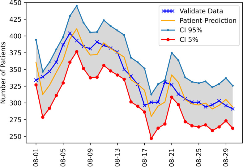
The ARIMA (2,2,2) forecasting value of the admitted patients with prediction confidential intervals (CI) between 5 and 95%
Fig. 5.

The ARIMAX (1, 1, 1) + X2 forecasting value of the admitted patients with prediction confidential intervals (CI) between 5 and 95%
The comparisons among forecasting models are shown in Tables 3, 4 and 5. The models numbered 12–17 in Table 2 are defined to be the baseline models. The models with x1 are the models numbered 29–34 while the models with x2 are the models numbered 46–51. The compared pairs were (baseline vs x1), (x1 vs x2), and (baseline vs x2). The comparison was done under the same parameter setting. The result of R,2 RMSE and MAE (Tables 3, 4 and 5) yielded a good result indicating that time forecasting models could improve correlation of determination when we added exogenous variables.
Table 3.
The comparison of Coefficient of determination (R2)
| No | R2 Comparison | All Wave | Wave 1 | Wave 2 | Wave 3 | Wave 4 | Wave 3–4 | ||||||
|---|---|---|---|---|---|---|---|---|---|---|---|---|---|
| Win | Loss | Win | Loss | Win | Loss | Win | Loss | Win | Loss | Win | Loss | ||
| 1 | baseline vs x1 | 3 | 3 | 6 | 0 | 1 | 5 | 5 | 1 | 0 | 6 | 6 | 0 |
| 2 | x1 vs x2 | 2 | 4 | 3 | 3 | 2 | 4 | 2 | 4 | 4 | 2 | 3 | 3 |
| 3 | baseline vs x2 | 4 | 2 | 6 | 0 | 0 | 6 | 4 | 2 | 4 | 2 | 4 | 2 |
| SUM | 9 | 9 | 15 | 3 | 3 | 15 | 11 | 7 | 8 | 10 | 13 | 5 | |
Table 4.
The comparison of Root mean square error (RMSE)
| No | RMSE Comparison | All Wave | Wave 1 | Wave 2 | Wave 3 | Wave 4 | Wave 3–4 | ||||||
|---|---|---|---|---|---|---|---|---|---|---|---|---|---|
| Win | Loss | Win | Loss | Win | Loss | Win | Loss | Win | Loss | Win | Loss | ||
| 1 | baseline vs x1 | 3 | 3 | 4 | 2 | 4 | 2 | 6 | 0 | 6 | 0 | 2 | 4 |
| 2 | x1 vs x2 | 4 | 2 | 4 | 2 | 3 | 3 | 2 | 4 | 5 | 1 | 1 | 5 |
| 3 | baseline vs x2 | 3 | 3 | 6 | 0 | 6 | 0 | 6 | 0 | 5 | 1 | 2 | 4 |
| SUM | 10 | 8 | 14 | 4 | 13 | 5 | 14 | 4 | 16 | 2 | 5 | 13 | |
Table 5.
The comparison of Mean Absolute error (MAE)
| No | MAE Comparison | All Wave | Wave 1 | Wave 2 | Wave 3 | Wave 4 | Wave 3–4 | ||||||
|---|---|---|---|---|---|---|---|---|---|---|---|---|---|
| Win | Loss | Win | Loss | Win | Loss | Win | Loss | Win | Loss | Win | Loss | ||
| 1 | baseline vs x1 | 3 | 3 | 4 | 2 | 3 | 3 | 6 | 0 | 6 | 0 | 2 | 4 |
| 2 | x1 vs x2 | 4 | 2 | 4 | 2 | 3 | 3 | 2 | 4 | 5 | 1 | 1 | 5 |
| 3 | baseline vs x2 | 3 | 3 | 6 | 0 | 5 | 1 | 6 | 0 | 5 | 1 | 2 | 4 |
| SUM | 10 | 8 | 14 | 4 | 11 | 7 | 14 | 4 | 16 | 2 | 5 | 13 | |
The predicted values, CI 5% (lower confidence interval) and CI 95% (upper confidence interval), and actual data of the models are shown in Table 6 and Fig. 4. In addition, the improved predictive values of the models by adding exogenous variables are shown in Table 7 and Fig. 5. For example, ARIMA (2, 2, 2) predicted that the number of cumulative confirmed cases for the next 30 days could be 291 to 334 cases. ARIMAX (1, 1, 1) + x2 predicted that the number of cumulative confirmed cases for the next 30 days could be 293–330 cases.
Table 6.
The number of patient prediction for time-series model ARIMA (2, 2, 2) + X2 Training from May 1 to July 22, 2021, Prediction from August 1 to August 30, 2021
| Date | Actual data | Prediction | Lower CI | Upper CI |
|---|---|---|---|---|
| August 1, 2021 | 334 | 361 | 327 | 394 |
| August 2, 2021 | 339 | 313 | 279 | 347 |
| August 3, 2021 | 347 | 326 | 292 | 361 |
| August 4, 2021 | 361 | 346 | 311 | 380 |
| August 5, 2021 | 387 | 364 | 330 | 398 |
| August 6, 2021 | 404 | 395 | 361 | 430 |
| August 7, 2021 | 393 | 411 | 377 | 445 |
| August 8, 2021 | 384 | 386 | 351 | 420 |
| August 9, 2021 | 381 | 371 | 337 | 405 |
| August 10, 2021 | 391 | 372 | 338 | 406 |
| August 11, 2021 | 386 | 390 | 356 | 424 |
| August 12, 2021 | 382 | 381 | 348 | 415 |
| August 13, 2021 | 376 | 375 | 342 | 408 |
| August 14, 2021 | 350 | 368 | 335 | 401 |
| August 15, 2021 | 340 | 335 | 302 | 368 |
| August 16, 2021 | 328 | 328 | 295 | 361 |
| August 17, 2021 | 296 | 319 | 286 | 352 |
| August 18, 2021 | 301 | 280 | 247 | 313 |
| August 19, 2021 | 301 | 295 | 262 | 328 |
| August 20, 2021 | 331 | 301 | 268 | 334 |
| August 21, 2021 | 327 | 342 | 309 | 375 |
| August 22, 2021 | 313 | 331 | 297 | 364 |
| August 23, 2021 | 306 | 305 | 272 | 338 |
| August 24, 2021 | 301 | 299 | 266 | 332 |
| August 25, 2021 | 301 | 297 | 264 | 330 |
| August 26, 2021 | 294 | 300 | 267 | 332 |
| August 27, 2021 | 297 | 291 | 259 | 323 |
| August 28, 2021 | 303 | 296 | 264 | 328 |
| August 29, 2021 | 296 | 305 | 273 | 337 |
| August 30, 2021 | 291 | 294 | 262 | 326 |
CI confidence interval
Table 7.
The number of patient prediction for time-series model ARIMAX (1,1,1) + X2 Training from May 1 to July 22, 2021, Prediction from August 1 to August 30, 2021
| Date | Actual data | Prediction | Lower CI | Upper CI |
|---|---|---|---|---|
| August 1, 2021 | 334 | 330 | 293 | 365 |
| August 2, 2021 | 339 | 333 | 296 | 368 |
| August 3, 2021 | 347 | 342 | 305 | 380 |
| August 4, 2021 | 361 | 345 | 307 | 382 |
| August 5, 2021 | 387 | 362 | 325 | 399 |
| August 6, 2021 | 404 | 391 | 353 | 428 |
| August 7, 2021 | 393 | 404 | 366 | 441 |
| August 8, 2021 | 384 | 385 | 348 | 422 |
| August 9, 2021 | 381 | 379 | 343 | 416 |
| August 10, 2021 | 391 | 377 | 341 | 414 |
| August 11, 2021 | 386 | 392 | 355 | 428 |
| August 12, 2021 | 382 | 380 | 344 | 416 |
| August 13, 2021 | 376 | 379 | 343 | 415 |
| August 14, 2021 | 350 | 371 | 336 | 407 |
| August 15, 2021 | 340 | 340 | 304 | 375 |
| August 16, 2021 | 328 | 338 | 302 | 373 |
| August 17, 2021 | 296 | 322 | 287 | 358 |
| August 18, 2021 | 301 | 290 | 250 | 321 |
| August 19, 2021 | 301 | 305 | 270 | 341 |
| August 20, 2021 | 331 | 298 | 263 | 333 |
| August 21, 2021 | 327 | 335 | 304 | 376 |
| August 22, 2021 | 313 | 321 | 285 | 356 |
| August 23, 2021 | 306 | 309 | 273 | 344 |
| August 24, 2021 | 301 | 304 | 269 | 339 |
| August 25, 2021 | 301 | 299 | 264 | 334 |
| August 26, 2021 | 294 | 301 | 266 | 335 |
| August 27, 2021 | 297 | 291 | 256 | 325 |
| August 28, 2021 | 303 | 298 | 264 | 332 |
| August 29, 2021 | 296 | 303 | 269 | 338 |
| August 30, 2021 | 291 | 293 | 259 | 327 |
CI confidence interval
Association rule mining
This section explores the association analysis when association rule mining is applied. We present significant rules for the data that included four attributes’ values in the dataset. Table 1 shows preliminary analysis of dataset that was extracted for a total of 3685 patients. The patient data consist of eleven attributes and 35 attribute values. In addition, an attribute code is defined for item set name and frequency of each attribute code. We extract 595 significant rules for the data.
The association rules grouped by four attributes related to managing hospital resources are shown in Table 8. Length of stay more than 14 days is related to healthcare workers and three underlying diseases other, pregnant, and dyslipidemia that have the same value of 1.017. Length of stay less than 14 give the interesting result on symptom mode (Lift of 6.464), three underlying diseases, and age more than 65 years old.
Table 8.
Top 5 association rules for different combinations of particular consequence, their Support, Average-confidence, Confidence (LHS ➔ RHS), Confidence (RHS ➔ LHS) and Lift measures
| No | LHS | RHS | N(A) | N(B) | N(A,B) | SupLR | ConfA | ConfLR | ConfRL | LiftLR |
|---|---|---|---|---|---|---|---|---|---|---|
| Length of Stay less than or equal to 14 days | ||||||||||
| 1 | job_health | los_1_14 | 93 | 3625 | 93 | 2.524 | 51.283 | 100.000 | 2.566 | 1.017 |
| 2 | ud_oth | los_1_14 | 64 | 3625 | 64 | 1.737 | 50.883 | 100.000 | 1.766 | 1.017 |
| 3 | ud_preg | los_1_14 | 23 | 3625 | 23 | .624 | 50.317 | 100.000 | .634 | 1.017 |
| 4 | ud_dlp | los_1_14 | 14 | 3625 | 14 | .380 | 50.193 | 100.000 | .386 | 1.017 |
| 5 | cxr_pneu | los_1_14 | 472 | 3625 | 470 | 12.754 | 56.271 | 99.576 | 12.966 | 1.012 |
| Length of Stay more than or equal to 15 days | ||||||||||
| 1 | sym_mode | los_15 | 19 | 60 | 2 | .054 | 6.930 | 10.526 | 3.333 | 6.465 |
| 2 | ud_meta | los_15 | 53 | 60 | 3 | .081 | 5.330 | 5.660 | 5.000 | 3.476 |
| 3 | ud_dm | los_15 | 18 | 60 | 1 | .027 | 3.611 | 5.556 | 1.667 | 3.412 |
| 4 | ud_ht | los_15 | 39 | 60 | 2 | .054 | 4.231 | 5.128 | 3.333 | 3.150 |
| 5 | age_65 | los_15 | 74 | 60 | 2 | .054 | 3.018 | 2.703 | 3.333 | 1.660 |
| Home Discharge | ||||||||||
| 1 | ud_ht | dc_home | 39 | 3600 | 39 | 1.058 | 50.542 | 100.000 | 1.083 | 1.024 |
| 2 | ud_dm | dc_home | 18 | 3600 | 18 | .488 | 50.250 | 100.000 | .500 | 1.024 |
| 3 | ud_dlp | dc_home | 14 | 3600 | 14 | .380 | 50.194 | 100.000 | .389 | 1.024 |
| 4 | age_24 | dc_home | 1148 | 3600 | 1131 | 30.692 | 64.968 | 98.519 | 31.417 | 1.008 |
| 5 | cxr_pneu | dc_home | 472 | 3600 | 465 | 12.619 | 55.717 | 98.517 | 12.917 | 1.008 |
| Refer to General hospital | ||||||||||
| 1 | sym_mode | dc_hosp | 19 | 85 | 4 | .109 | 12.879 | 21.053 | 4.706 | 9.127 |
| 2 | ud_preg | dc_hosp | 23 | 85 | 3 | .081 | 8.286 | 13.043 | 3.529 | 5.655 |
| 3 | ud_meta | dc_hosp | 53 | 85 | 6 | .163 | 9.190 | 11.321 | 7.059 | 4.908 |
| 4 | los_15 | dc_hosp | 60 | 85 | 5 | .136 | 7.108 | 8.333 | 5.882 | 3.613 |
| 5 | age_65 | dc_hosp | 74 | 85 | 6 | .163 | 7.583 | 8.108 | 7.059 | 3.515 |
| Chest X-ray is No lesion | ||||||||||
| 1 | job_health | cxr_no | 93 | 3213 | 91 | 2.469 | 50.341 | 97.849 | 2.832 | 1.122 |
| 2 | source_hosp | cxr_no | 91 | 3213 | 88 | 2.388 | 49.721 | 96.703 | 2.739 | 1.109 |
| 3 | age_24 | cxr_no | 1148 | 3213 | 1058 | 28.711 | 62.545 | 92.160 | 32.929 | 1.057 |
| 4 | symp_ast | cxr_no | 2295 | 3213 | 2112 | 57.313 | 78.880 | 92.026 | 65.733 | 1.055 |
| 5 | ud_repp | cxr_no | 82 | 3213 | 73 | 1.981 | 45.648 | 89.024 | 2.272 | 1.021 |
| Chest X-ray is Pneumonia | ||||||||||
| 1 | sym_mode | cxr_pneu | 19 | 472 | 8 | .217 | 21.900 | 42.105 | 1.695 | 3.287 |
| 2 | age_65 | cxr_pneu | 74 | 472 | 31 | .841 | 24.230 | 41.892 | 6.568 | 3.271 |
| 3 | ud_ht | cxr_pneu | 39 | 472 | 11 | .299 | 15.268 | 28.205 | 2.331 | 2.202 |
| 4 | ud_dm | cxr_pneu | 18 | 472 | 5 | .136 | 14.419 | 27.778 | 1.059 | 2.169 |
| 5 | ud_meta | cxr_pneu | 53 | 472 | 14 | .380 | 14.691 | 26.415 | 2.966 | 2.062 |
| Current incidence in Wave 1 | ||||||||||
| 1 | los_15 | wave_1 | 60 | 55 | 13 | .353 | 22.652 | 21.667 | 23.636 | 14.517 |
| 2 | source_hosp | wave_1 | 91 | 55 | 16 | .434 | 23.337 | 17.582 | 29.091 | 11.780 |
| 3 | job_health | wave_1 | 93 | 55 | 15 | .407 | 21.701 | 16.129 | 27.273 | 10.806 |
| 4 | dc_hosp | wave_1 | 85 | 55 | 6 | .163 | 8.984 | 7.059 | 10.909 | 4.729 |
| 5 | symp_ast | wave_1 | 2295 | 55 | 54 | 1.465 | 50.267 | 2.353 | 98.182 | 1.576 |
| Current incidence in Wave 2 | ||||||||||
| 1 | job_health | wave_2 | 93 | 311 | 13 | .353 | 9.079 | 13.978 | 4.180 | 1.656 |
| 2 | symp_ast | wave_2 | 2295 | 311 | 266 | 7.218 | 48.560 | 11.590 | 85.531 | 1.373 |
| 3 | source_hosp | wave_2 | 91 | 311 | 10 | .271 | 7.102 | 10.989 | 3.215 | 1.302 |
| 4 | bmi_25_29 | wave_2 | 931 | 311 | 96 | 2.605 | 20.590 | 10.311 | 30.868 | 1.222 |
| 5 | bmi_30 | wave_2 | 445 | 311 | 42 | 1.140 | 11.472 | 9.438 | 13.505 | 1.118 |
| Current incidence in Wave 3 | ||||||||||
| 1 | symp_ast | wave_3 | 2295 | 1779 | 1285 | 34.871 | 64.111 | 55.991 | 72.232 | 1.160 |
| 2 | age_25_44 | wave_3 | 1838 | 1779 | 1009 | 27.381 | 55.807 | 54.897 | 56.717 | 1.137 |
| 3 | cxr_no | wave_3 | 3213 | 1779 | 1635 | 44.369 | 71.396 | 50.887 | 91.906 | 1.054 |
| 4 | ud_none | wave_3 | 3392 | 1779 | 1700 | 46.133 | 72.839 | 50.118 | 95.559 | 1.038 |
| 5 | bmi_25 | wave_3 | 2309 | 1779 | 1136 | 30.828 | 56.527 | 49.199 | 63.856 | 1.019 |
| Current incidence in Wave 4 | ||||||||||
| 1 | ud_preg | wave_4 | 23 | 1540 | 22 | .597 | 48.540 | 95.652 | 1.429 | 2.289 |
| 2 | ud_dm | wave_4 | 18 | 1540 | 17 | .461 | 47.774 | 94.444 | 1.104 | 2.260 |
| 3 | age_65 | wave_4 | 74 | 1540 | 64 | 1.737 | 45.321 | 86.486 | 4.156 | 2.069 |
| 4 | ud_meta | wave_4 | 53 | 1540 | 43 | 1.167 | 41.962 | 81.132 | 2.792 | 1.941 |
| 5 | sym_mode | wave_4 | 19 | 1540 | 15 | .407 | 39.961 | 78.947 | .974 | 1.889 |
The interesting rule of discharge had two value attributes. The result showed that referral to hospitals was strongly related to symptom of Mode (Lift of 9.127). In addition, four features in this attribute showed high Lift values; underlying diseases (5.655), metabolic syndrome (4.098), length of stay more than 14 days (3.613), and age more than 65 years old (5.515). Chest x-ray with no lesion presented the same level of Lift. However, two features which showed high numbers of patients were age less than 24 years old (1148) and symptom asymptomatic (2295). Moreover, chest x-ray with pneumonia showed all high interesting value Symptom of Mode (3.287), age more than 65 (3.271), underlying diseases diabetes mellitus (2.169), and underlying diseases Metabolic (2.062). In current incident, Wave 1 showed high interest on Length of stay more than 14-days and source of infection from hospital and healthcare worker patients. Wave 2 was also related to healthcare worker, asymptomatic and source of infection from hospital, as was Wave 3. In Wave 4, underlying diseases, age more than 65 and symptom mode showed strong relationships. Association rules selected key attributes of the data set to be exogenous variables of a time series analysis.
Discussion
The first wave of SARS-CoV-2 occurred in early 2020, and the second, third and fourth waves rapidly spread from early to mid-2021, representing an unprecedented phenomenon in medical services, society and the economy of Thailand. The number of COVID-19 patients shown in this study increased from the first wave of just 55 patients to 311, 1779 and 1540 in the second, third and fourth waves, respectively, which evolved more than 30 times of the total number of patients admitted at the field hospital. Most of patients were at least 44 years old and were predominantly female. Patients included in this study were mostly asymptomatic and had no sign of pneumonia in the chest x-ray due to the field hospital system’s focus on patients who did not require advanced treatment. But during the third and fourth waves, the number of mild to moderate symptoms with pneumonia of COVID-19 patients significantly increased because of the greater severity of the delta variant of SARS-COV-2. The huge number of patients was a burden on the limited resources of Thailand’s healthcare system. Therefore, this study presented the use of time series modeling and association rule mining to forecast the COVID-19 pandemic outbreak as well as to analyze its associated prognostic factors. The method presented a data-oriented approach that applies time-series analysis and association analysis to reveal meaningful hidden patterns for efficient handling of another pandemic crisis.
ARIMA models have been successfully applied for predicting the disease outbreak. Several studies have utilized the ARIMA model to forecast the spread of COVID-19 in many countries including the US, Brazil, India, Russia and Spain [28, 29]. The studies using ARIMA models to predict COVID-19 cases relative to total confirmed cases presented an average RMSE of 144.81 across 6 geographic regions [28], MAE of 787 to 1506 in USA and 82 to 570 in Italy [18], and MAE of 2967 in Indonesia [20]. In this work, ARIMA (2, 2, 2) was selected as the most accurate ARIMA model for predicting the number of admitted COVID-19 cases in the field hospital, which achieved a R2 = 0.5695, RMSE = 29.7605, MAE = 27.5102 (Fig. 4). The forecast results of admitted cases on August 15 and August 30, 2021 were 335 and 294, respectively. In comparison with the actual values reported on the same dates, the forecasted values of our selected ARIMA model were within the upper and lower bounds at 95% confidence intervals. This signified an acceptable accuracy of this model for estimating admitted cases in the field hospital.
ARM is a structured method of discovering frequent patterns in a data set and forming noticeable rules among regular patterns. In the COVID-19 crisis, many nations, including Thailand, have a highest priority to save lives and protect their economies. A previous study using ARM for mining COVID-19 data to analyze factors related to COVID-19 situation management showed that face mask mandates combined with mobility reduction through moderate stay-at-home orders were most effective in reducing the number of COVID-19 cases in United State [24]. In this study, the ARM technique was used to analyze and identify factors related to the length of stay and prognosis of COVID-19 patients and found that the top five factors related to hospital stays longer than 14 days consisted of healthcare workers uncommon underlying diseases such as thalassemia, thyroid diseases, gout and G6PD deficiency, pregnant patients, dyslipidemia and signs of pneumonia in chest x-rays. This study also identified a clinical factor rule related to the worsening condition of the inpatient. Among those who needed more advanced medical treatment, the rules included mild to moderate COVID-19 symptoms, pregnant patients, metabolic syndrome, length of hospital stay more than 14 days, and patients older than 65 years old. These factors are consistent with those in a previous study, which reported similar conditions among patients who had a poor prognosis in COVID-19 infections [1, 30].
In any prediction tasks, more data is needed to achieve better performance from the models. This study developed the combination of the ARM technique and the ARIMA model, as the ARIMAX model. This model worked by selecting the rules related to COVID-19 prognosis from the ARM technique, including mild to moderate COVID-19 symptoms, patients with metabolic syndrome and patients older than 65 years old, and integrating them to the ARIMA model. Experimental results showed that the ARIMAX model (1, 1, 1) improved the accuracy of forecasting the number of admitted COVID-19 cases, which achieved a R2 = 0.5695, RMSE = 27.7508, MAE = 23.4642 (Fig. 5). The forecast value of this model for August 30, 2021 was estimated to be 259 to 327 cases. The actual number of cases on the same date was 291 cases. The actual value also was within the lower and upper prediction bounds for both 95% confidence intervals. To the best of our knowledge, this is the first study to combine the ARM technique with the ARIMA model for forecasting the COVID-19 cases by integrating the optimal exogenous variables from the ARM rules to form a predictive model. This ARIMAX model had the potential to predict the number of COVID-19 patients, which could be one of the reliable forecasting-based models for the future outbreak. These predictive models are intended to help better decision-making to plan an effective management system if the virus outbreak has not subsided.
Limitations
The limitation of this study is that the dataset was based on retrospective data from a single COVID-19 field hospital in Thailand with a limited number of cases and clinical variables of COVID-19 patients.
Future directions
In future work, the collaboration between multi-medical centers for a larger number and different variables of COVID-19 cases, including the medical records of clinical, laboratory and treatment data from various COVID-19 centers, would upgrade the forecasting performance of this AI model to predict the COVID-19 event more accurately. Additionally, geographic data related to the pandemic area could be used as a variable for alternative time series models such as space-time ARIMA models [31], which could be more reliable in predicting future COVID-19 outbreaks.
Conclusion
This study demonstrated that the ARIMAX model has the potential to increase the accuracy for predicting the number of COVID-19 cases by incorporating the most associated prognostic factors identified by ARM technique to the ARIMA model. The result of this study proved to be an effective AI model to predict the number of and to identify prognostic factors of admitted COVID-19 patients. This work is expected to be a novel AI-based decision-making model for preparation, organizing hospital resources and more optimal use of medical personnel and equipment to enhance healthcare decision-making, and to manage the COVID-19 pandemic but as well as other epidemic crises.
Acknowledgements
The authors would like to thank Supasek Sanmano from Thammasat Field Hospital and Kunch Ringrod from Thai Network for Disaster Resilience (TNDR) for data preparation. We thank Mr. Terrance J. Downey, English Editor for Thammasat University Office of Research and Innovation for English language editing.
Abbreviations
- COVID-19
Coronavirus disease 2019
- SARS-CoV-2
Severe Acute Respiratory Syndrome-Coronavirus-2
- MERS-CoV
Middle East Respiratory Syndrome Coronavirus
- CBC
Complete blood count
- LFTs
Liver function tests
- BUN
Balance urine nitrogen
- Cr
Creatinine
- SpO2
Pulse oxygen saturation
- BT
Body temperature
- BMI
Body mass index
- G6PD
Glucose-6-Phosphate Dehydrogenase
- ANN
Artificial Neural Network
- SVM
Support Vector Machine
- ARM
Association Rule Mining
- ARIMA
Auto Regressive Integrated Moving Average
- ARIMAX
Autoregressive Integrated Moving Average with Exogenous Covariates
- R2
Coefficient of determination
- RMSE
Root mean square error
- MAE
Mean absolute error
- CI
Confidence intervals
Authors’ contributions
Conceptualization: K.W., S.N., S.S.; Methodology: R.S., K.W., T.T., S.S.; Formal analysis and investigation: R.S., K.W., W.A., W.P., T.T., S.S.; Fund acquisition: W.A., T.T; Writing - original draft preparation: K.W., S.S.; Writing - review and editing: K.W., S.S.; Resources: W.A., C.M., K.M., K.S.; Supervision: S.S., S.N. All authors have read and agreed to the published version of the manuscript.
Funding
This work was supported by the Thammasat University Research Fund (CovidTU-03/2564), Center of Excellence in Intelligent Informatics, Speech and Language Technology and Service Innovation (CILS), and Intelligent Informatics and Service Innovation (IISI).
Availability of data and materials
The datasets used and/or analyzed during the current study are available from the corresponding author on reasonable requests.
Declarations
Ethics approval and consent to participate
The study protocol and the exempt from the need to obtain informed consent was approved by the Ethics Committee of the Thammasat University (COE 008/2564) in accordance with the 1964 Declaration of Helsinki.
Consent for publication
Not applicable.
Competing interests
The authors declare no competing interests.
Footnotes
Publisher’s Note
Springer Nature remains neutral with regard to jurisdictional claims in published maps and institutional affiliations.
Contributor Information
Rachasak Somyanonthanakul, Email: ratchasak.s@rsu.ac.th.
Kritsasith Warin, Email: warin@tu.ac.th.
Watchara Amasiri, Email: awatchar@engr.tu.ac.th.
Karicha Mairiang, Email: khunpa_kiki@hotmail.com.
Chatchai Mingmalairak, Email: michatch@staff.tu.ac.th.
Wararit Panichkitkosolkul, Email: wararit@tu.ac.th.
Krittin Silanun, Email: krittinsilanun@gmail.com.
Thanaruk Theeramunkong, Email: thanaruk@siit.tu.ac.th.
Surapon Nitikraipot, Email: suraniti@tu.ac.th.
Siriwan Suebnukarn, Email: ssiriwan@tu.ac.th.
References
- 1.Huang C, Wang Y, Li X, Ren L, Zhao J, Hu Y, Zhang L, Fan G, Xu J, Gu X, et al. Clinical features of patients infected with 2019 novel coronavirus in Wuhan, China. Lancet. 2020;395(10223):497–506. doi: 10.1016/S0140-6736(20)30183-5. [DOI] [PMC free article] [PubMed] [Google Scholar]
- 2.Wolkewitz M, Puljak L. Methodological challenges of analysing COVID-19 data during the pandemic. BMC Med Res Methodol. 2020;20(1):81. doi: 10.1186/s12874-020-00972-6. [DOI] [PMC free article] [PubMed] [Google Scholar]
- 3.Tao K, Tzou PL, Nouhin J, Gupta RK, de Oliveira T, Kosakovsky Pond SL, Fera D, Shafer RW. The biological and clinical significance of emerging SARS-CoV-2 variants. Nat Rev Genet. 2021;22(12):757–773. doi: 10.1038/s41576-021-00408-x. [DOI] [PMC free article] [PubMed] [Google Scholar]
- 4.World Health Organization . COVID-19 Weekly Epidemiological Update, Edition 95. 2022. [Google Scholar]
- 5.Yoo I, Alafaireet P, Marinov M, Pena-Hernandez K, Gopidi R, Chang JF, Hua L. Data mining in healthcare and biomedicine: a survey of the literature. J Med Syst. 2012;36(4):2431–2448. doi: 10.1007/s10916-011-9710-5. [DOI] [PubMed] [Google Scholar]
- 6.Huang F, Wang S, Chan C. 2012 IEEE International Conference on Granular Computing: 11–13 Aug. 2012. 2012. Predicting disease by using data mining based on healthcare information system; pp. 191–194. [Google Scholar]
- 7.Koh HC, Tan G. Data mining applications in healthcare. J Healthc Inf Manag. 2005;19(2):64–72. [PubMed] [Google Scholar]
- 8.Kriston L. Predictive accuracy of a hierarchical logistic model of cumulative SARS-CoV-2 case growth until May 2020. BMC Med Res Methodol. 2020;20(1):278. doi: 10.1186/s12874-020-01160-2. [DOI] [PMC free article] [PubMed] [Google Scholar]
- 9.Ayatollahi H, Gholamhosseini L, Salehi M. Predicting coronary artery disease: a comparison between two data mining algorithms. BMC Public Health. 2019;19(1):448. doi: 10.1186/s12889-019-6721-5. [DOI] [PMC free article] [PubMed] [Google Scholar]
- 10.Alfisahrin SNN, Mantoro T. 2013 International Conference on Advanced Computer Science Applications and Technologies: 23–24 Dec. 2013. 2013. Data Mining Techniques for Optimization of Liver Disease Classification; pp. 379–384. [Google Scholar]
- 11.Al-Turaiki I, Alshahrani M, Almutairi T. Building predictive models for MERS-CoV infections using data mining techniques. J Infect Public Health. 2016;9(6):744–748. doi: 10.1016/j.jiph.2016.09.007. [DOI] [PMC free article] [PubMed] [Google Scholar]
- 12.Abonazel M, Ibrahim A. Forecasting Egyptian GDP using ARIMA models. Rep Econ Finance. 2019;5:35–47. doi: 10.12988/ref.2019.81023. [DOI] [Google Scholar]
- 13.Cryer JD, Chan K-S. Time series analysis with applications in R, 2nd 2008. Edn. New York: Springer New York; 2008. [Google Scholar]
- 14.Zaki MJ. Scalable algorithms for association mining. IEEE Trans Knowl Data Eng. 2000;12(3):372–390. doi: 10.1109/69.846291. [DOI] [Google Scholar]
- 15.Heisterkamp SH, Dekkers AL, Heijne JC. Automated detection of infectious disease outbreaks: hierarchical time series models. Stat Med. 2006;25(24):4179–4196. doi: 10.1002/sim.2674. [DOI] [PubMed] [Google Scholar]
- 16.Zhang GP. Time series forecasting using a hybrid ARIMA and neural network model. Neurocomputing. 2003;50:159–175. doi: 10.1016/S0925-2312(01)00702-0. [DOI] [Google Scholar]
- 17.Abonazel M, Darwish N. Forecasting confirmed and recovered Covid-19 cases and deaths in Egypt after the genetic mutation of the virus: ARIMA box-Jenkins approach. Commun Math Biol Neurosci. 2022;2022:17. [Google Scholar]
- 18.Gecili E, Ziady A, Szczesniak RD. Forecasting COVID-19 confirmed cases, deaths and recoveries: revisiting established time series modeling through novel applications for the USA and Italy. PLoS One. 2021;16(1):e0244173. doi: 10.1371/journal.pone.0244173. [DOI] [PMC free article] [PubMed] [Google Scholar]
- 19.Singh S, Parmar KS, Makkhan SJS, Kaur J, Peshoria S, Kumar J. Study of ARIMA and least square support vector machine (LS-SVM) models for the prediction of SARS-CoV-2 confirmed cases in the most affected countries. Chaos, Solitons Fractals. 2020;139:110086. doi: 10.1016/j.chaos.2020.110086. [DOI] [PMC free article] [PubMed] [Google Scholar]
- 20.Aditya Satrio CB, Darmawan W, Nadia BU, Hanafiah N. Time series analysis and forecasting of coronavirus disease in Indonesia using ARIMA model and PROPHET. Proc Comput Sci. 2021;179:524–532. doi: 10.1016/j.procs.2021.01.036. [DOI] [Google Scholar]
- 21.Agrawal R, Imieliński T, Swami A. Proceedings of the 1993 ACM SIGMOD international conference on management of data. Washington, D.C.: Association for Computing Machinery; 1993. Mining association rules between sets of items in large databases; pp. 207–216. [Google Scholar]
- 22.K S L, G DV: Extracting association rules from medical health records using multi-criteria decision analysis. Proc Comput Sci 2017, 115:290–295.
- 23.Tandan M, Acharya Y, Pokharel S, Timilsina M. Discovering symptom patterns of COVID-19 patients using association rule mining. Comput Biol Med. 2021;131:104249. doi: 10.1016/j.compbiomed.2021.104249. [DOI] [PMC free article] [PubMed] [Google Scholar]
- 24.Katragadda S, Gottumukkala R, Bhupatiraju RT, Kamal AM, Raghavan V, Chu H, Kolluru R, Ashkar Z. Association mining based approach to analyze COVID-19 response and case growth in the United States. Sci Rep. 2021;11(1):18635. doi: 10.1038/s41598-021-96912-5. [DOI] [PMC free article] [PubMed] [Google Scholar]
- 25.Amasiri W, Warin K, Mairiang K, Mingmalairak C, Panichkitkosolkul W, Silanun K, et al. Analysis of characteristics and clinical outcomes for crisis management during the four waves of the COVID-19 pandemic. Int J Environ Res Public Health. 2021;18(23):12633. [DOI] [PMC free article] [PubMed]
- 26.Time Series Models AR, MA, ARMA, ARIMA; 2020 [cited 2021 7 December] Available from: https://towardsdatascience.com/time-series-models-d9266f8ac7b0.
- 27.Barnston AG. Correspondence among the correlation, RMSE, and Heidke forecast verification measures; refinement of the Heidke score. Weather Forecast. 1992;7(4):699–709. doi: 10.1175/1520-0434(1992)007<0699:CATCRA>2.0.CO;2. [DOI] [Google Scholar]
- 28.Hernandez-Matamoros A, Fujita H, Hayashi T, Perez-Meana H. Forecasting of COVID19 per regions using ARIMA models and polynomial functions. Appl Soft Comput. 2020;96:106610. doi: 10.1016/j.asoc.2020.106610. [DOI] [PMC free article] [PubMed] [Google Scholar]
- 29.Darapaneni N, Reddy D, Paduri AR, Acharya P, Nithin HS. 2020 11th IEEE Annual Ubiquitous Computing, Electronics & Mobile Communication Conference (UEMCON): 28–31 Oct. 2020. 2020. Forecasting of COVID-19 in India Using ARIMA Model; pp. 0894–0899. [Google Scholar]
- 30.Noor FM, Islam MM. Prevalence and associated risk factors of mortality among COVID-19 patients: a Meta-analysis. J Community Health. 2020;45(6):1270–1282. doi: 10.1007/s10900-020-00920-x. [DOI] [PMC free article] [PubMed] [Google Scholar]
- 31.Awwad FA, Mohamoud MA, Abonazel MR. Estimating COVID-19 cases in Makkah region of Saudi Arabia: space-time ARIMA modeling. PLoS One. 2021;16(4):e0250149. doi: 10.1371/journal.pone.0250149. [DOI] [PMC free article] [PubMed] [Google Scholar]
Associated Data
This section collects any data citations, data availability statements, or supplementary materials included in this article.
Data Availability Statement
The datasets used and/or analyzed during the current study are available from the corresponding author on reasonable requests.