Abstract
The pandemic outbreak of severe acute respiratory syndrome caused by the Coronavirus 2 disease in 2019, also known as SARS-COV-2 and COVID-19, has claimed over 5.6 million lives till now. The highly infectious nature of the Covid-19 virus has resulted into multiple massive upsurges in counts of new infections termed as ‘waves.’ These waves consist of numerous rising and falling counts of Covid-19 infection cases with changing dates that confuse analysts and researchers. Due to this confusion, the detection of emergence or drop of Covid waves is currently a subject of intensive research. Hence, we propose an algorithmic framework to forecast the upcoming details of Covid-19 infection waves for a region. The framework consists of a displaced double moving average (DMA) algorithm for forecasting the start, rise, fall, and end of a Covid-19 wave. The forecast is generated by detection of potential dates with specific counts called ‘markers.’ This detection of markers is guided by decision rules generated through rough set theory. We also propose a novel ‘corrected moving average’ (SMA) technique to forecast the upcoming count of new infections in a region. We implement our proposed framework on a database of Covid-19 infection specifics fetched from 12 countries, namely: Argentina, Colombia, New Zealand, Australia, Cuba, Jamaica, Belgium, Croatia, Libya, Kenya, Iran, and Myanmar. The database consists of day-wise time series of new and total infection counts from the date of first case till 31st January 2022 in each of the countries mentioned above. The DMA algorithm outperforms other baseline techniques in forecasting the rise and fall of Covid-19 waves with a forecast precision of 94.08%. The SMA algorithm also surpasses its counterparts in predicting the counts of new Covid-19 infections for the next day with the least mean absolute percentage error (MAPE) of 36.65%. Our proposed framework can be deployed to forecast the upcoming trends and counts of new Covid-19 infection cases under a minimum observation window of 7 days with high accuracy. With no perceptible impact of countermeasures on the pandemic until now, these forecasts will prove supportive to the administration and medical bodies in scaling and allotment of medical infrastructure and healthcare facilities.
Keywords: Covid-19, Moving average, Rough set, Pandemic, Forecast
1. Introduction
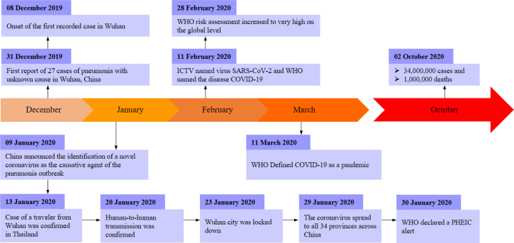
Will there be a next Covid wave? This question has been haunting human civilization since December 2019, when the Coronavirus disease emerged in the Hubei central province of China [1]. By the end of January 2020, the World Health Organization (WHO) declared Covid-19 a Public Health Emergency of International Concern (PHEIC) (Fig. 1). Since then, Covid-19 has evolved as a severe global pandemic that has instigated unprecedented havoc around the globe [2]. In the current state, the highly contagious Covid-19 virus attacks the human respiratory system causing severe health issues and even death.
Fig. 1.
Timeline of Covid-19 pandemic [1].
To date, the changing counts of Covid-19 infections in the population of every country are being regularly recorded. Several variants [3] of the Coronavirus have instigated numerous spikes and drops in these infection counts for multiple times in various regions of the world. At times, these spikes and drops together compose patterns of extreme upsurges and downturns for a noticeable period causing severe damage to lives and resources. Such patterns of infection counts and their behaviors have been termed as waves of the Covid-19 pandemic [4]. However, the spikes and drops are regularly witnessed phenomena in the recorded infection counts during waves as well as moderate periods. Therefore, distinguishing a temporary spike or a group of spikes in infection counts from an upcoming wave is a challenge. Ignorance of an approaching infection wave as a transitory spike can lead to discrepancies like underprepared infrastructure and lousy precautionary measures. Similarly, confusing a minor drop in counts with a downturn of the wave may lead to inconsistencies like a premature discharge of treatment and safeguards. Eventually, such inconsistencies result in a drastic loss of lives due to waves of new Covid-19 infections.
In this scenario, a well-defined demarcation of an upsurge or a downfall in a Covid-19 infection wave from temporary spikes or drops in the counts is critically essential. Hence, we propose an approach for detecting marker points among these spikes and drops. These markers enable us to forecast the behavior of an upcoming or ongoing wave of new infections with an observation window of minimum 7 days.
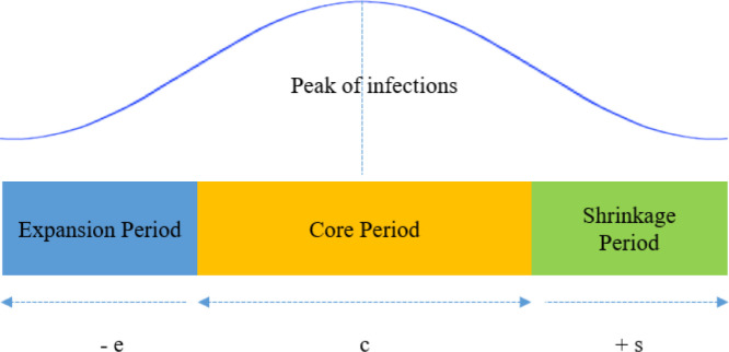
On a general note, the duration of a wave leads from an expansion period to a core and ends up with a shrinkage period (Fig. 2). The points where the expansion and shrinkage of wave initiates can be termed as up-trigger and down-trigger, respectively. Similarly, all points of rise in counts can be labeled as spikes, while the points of fall can be depicted as drops.
Fig. 2.
The general structure of a wave.
In this paper, we signify these triggers, spikes, and drops under a collective term called ‘marker.’ Detection of these markers will play a conclusive role in estimating the rise and fall of Covid waves in our proposed work. This estimation of each marker can be utilized for forecasting a specific behavior of Covid-19 waves (Table 1).
Table 1.
Markers and their forecast interpretations.
| Marker | Notation | Forecasted result |
|---|---|---|
| Up trigger | Start of a new wave | |
| Down trigger | End of an ongoing wave | |
| Spike | s | Rise in an existing wave |
| Drop | d | Fall of an existing wave |
At the time of writing of this manuscript, the Omicron variant [5] of Covid-19 infection has surpassed all previous records of infection cases triggering at least the third or fourth wave of infections in over 200 countries worldwide. Each wave of infections is composed of numerous temporary rises and falls in the infection counts. These rises and falls create a lack of transparency and generate severe confusion about the upcoming state of this pandemic. This confusion eventually worsens the situation and leads to the next wave of infections causing further damage. Thus, intensive research efforts are going on for cure [6], [7], detection [8], and prevention [9] of Covid-19 disease. However, despite these efforts, any perceptible impact on this disease is unclear. This state of affairs has also motivated researchers to predict the upcoming state of Covid-19 in different regions of the world. Several works have been proposed on the forecast of infection counts [10] and duration of infection [11] within a brief span of time.
From simple iterations of confirmed cases [12] to dedicated computational models have been proposed for the projection and forecast of Covid-19 disease. The Susceptible–Infectious–Recovered–Dead (SIDR) model proposed by Fanelli et al. [13] employs a differential evolution algorithm for simulating the mean-field kinetics of the epidemic spread. Estimation of the basic reproduction number, case fatality, and case recovery ratios by Anastassopoulou et al. [14] is a further calibrated elaboration of such a model. Another instance of similar computational models is the SARIIS model presented by Sarkar, Khajanchi & Nieto [15]. SARIIS partitions the count of confirmed cases into susceptible (S), asymptomatic (A), recovered (R), infected (I), isolated infected (), and quarantined susceptible (S) compartments to generate forecasts. A major section of the works on the Covid-19 forecast employs ARIMA modeling for [11], [16] predicting upcoming counts in the future. Here, the researchers utilize the predictive performance of ARIMA models for projecting the specifics of Coronavirus infection in a region for a given span.
However, as stated earlier, a wave of Covid-19 infections involves multiple sudden bursts of numbers. The inefficiency in handling these sudden data bursts is a significant limitation of ARIMA models [17]. ARIMA models generate linear patterns by corrective incremental adjustments over the autoregressive characteristics of the time series data. Such linear patterns generally fail to predict time series data that include multiple turning points [11]. Also, the dynamics of geography, climate, demography, and culture lay a serious impact on the behavior of a disease in a region. Likewise, the financial condition of the population, medical infrastructure, and especially the testing facilities play a decisive role in the epidemiological impression of the virus spread. Any mechanism that predicts on the basis of these fluctuating factors will be vulnerable to inconsistencies.
Furthermore, the proposed works stated in this section project the infection cases as a cumulative function of the factors discussed above. Only a few of them emphasize the temporal changes in the infection counts for an upcoming period. This fact also limits their efficiency in predicting the behavior of a wave of infection cases.
Therefore, we propose a framework of algorithms to forecast the behavior of a wave by detecting specific counts of new infections in a Covid-19 time series. We also propose to forecast the upcoming count of new Covid infections for the next day in a region.
1.1. Paper’s contributions
The contributions of the proposed work can be summarized as follows:
Wave behavior forecast: We propose an algorithmic procedure to forecast the rise and fall of a potential wave of new infections by detecting the markers present in the timeline of Covid-19 infection cases in a provided region with an average forecast precision of 94.08%.
The procedure comprises a displaced double moving average ( DMA) technique and a decimal base shift function (). The displaced double moving average ( DMA) generates the trend underlying a Covid-19 infection wave. By utilizing this trend, the decimal base shift () detects changes in infection counts that can be identified as potential markers of rise and fall in a wave of new infections. The determination of markers is guided by decision rules derived from the implementation of the rough set theory process on the Covid-19 time series data. These markers are later interpreted to forecast the upcoming behavior of a Covid-19 wave.
Infection count forecast: We further propose a novel algorithm for forecasting the upcoming counts of new infection cases in a time series data. The proposed algorithm is a variant of the single moving average method corrected by the addition of error gaps between the actual and projected values. Hence, we have named it as ‘corrected single moving average ( SMA)’ technique.
A framework of the algorithms proposed above has been implemented on time series data of new Covid-19 infections recorded in 12 different countries. We employ the walk-forward approach [18] for the execution of this framework on the time series data. This implies that the results of the proposed models get updated at every next input of new infection counts. The proposed work can be employed for the estimation of upcoming specifics of Covid-19 infections in a geographical region with an observation window period of 7 to 14 days.
1.2. Literature referenced
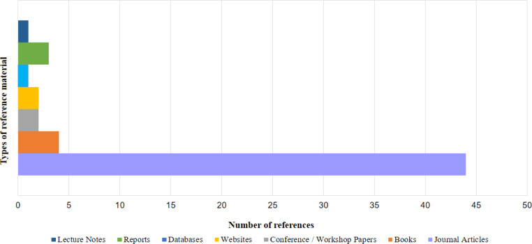
We have exhaustively referenced a sizable volume of literature from an extensive range of research works. Among these works, the ones based on the Covid-19 pandemic have been published from January 2020 to February 2022. The literature predominantly comprises reports, databases, lecture notes, websites, and books. But the chief constituent of this literature entails research articles from conferences and journals belonging to domains of computing, statistics, and medical expertise. The kinds and volume percentages of the different constituents of this literature have been summarized into a visualization presented in Fig. 3. The literature is entirely available in the public domain, and therefore no conflicts of interest have been discovered.
Fig. 3.
Type and percentage of research literature referenced in this work.
1.3. Paper’s outline
The structure of the paper is as follows:
The literature background constituting the essential concepts and terminologies has been presented in Section 2.
Section 3 covers the problem statement, notations, data description, and formulated techniques under the proposed work.
Implementation of proposed techniques along with a case study of the first wave of Covid-19 pandemic in Australia is elaborated in Section 4.
Performance measures as well the analysis of results has been conferred over in Section 5.
Section 6 discusses various dimensions and assessments of the proposed approach.
The paper concludes with a summary of the proposed work and directions of possible future research.
2. Background
Before moving forward, we now discuss the prospective technical approaches that will serve as conceptual blocks for the design and development of the proposed forecast models. The architecture of these models is composed of moving average approach. A double moving average (DMA) variant of this approach combined with rough set-based decision rules is used for the detection of markers in a Covid wave. Likewise, a single moving average variant has been employed to forecast the infection counts for the next day. Thus, in this section, we discuss the specifics of rough sets and moving averages that comprise the architecture of the proposed forecast models.
2.1. Rough sets
Rough set theory can be viewed as a soft computing approach of uncertainty mathematics for mining structural patterns within incomplete, imprecise, and inexact information [19], [20]. The concept of rough sets was introduced by Zdzislaw I. Pawlak in his landmark paper in the year 1982 [21]. A rough set is a generalization of classical set theory researched on the logical characteristics of information systems. They have been successfully applied in problem domains such as pattern mining, feature extraction, feature selection, and decision rule generation. Here we discuss a few definitions regarding the rough set theory relevant to our proposed approach.
Definition 1 Information Systems —
The rough set theory suggests the storage of input data in tabular designs called information systems. Each tuple of this information system represents a fact or an object which may be inconsistent with each other. Mathematically, any information system is expressed as a pair (U, C) where:
U (universe) a non-empty finite set of all objects from the problem domain
C (attribute) a non-empty finite set of conditional attributes such that U holds for every attribute c C. Here should be considered the value set of attribute ‘c’.
Definition 2 Indiscernibility —
Indiscernibility can be stated as the similarity of a set of attribute values for 2 or more given objects. As presented above, the information system table may consist of multiple objects (records) stored with similar feature values. Reducing the number of objects in this table can improve the efficiency of a proposed computational model. This reduction can be implemented by storing only the representative objects of every set with common features. Such representative objects are termed as indiscernible objects. Here, indiscernibility can be stated as an equivalence relation for the identification of these representative or identical objects.
Mathematically, for a set of attributes P Q, an indiscernibility relation IND(P) can be presented as:
This implies that the 2 objects x and y will be indiscernible by the set P of attributes in set Q, if p(x) p(y) for every attribute p P.
The sets of attributes that are indiscernible are also termed as elementary sets.
Definition 3 Formal Approximations —
We have discussed earlier that the rough set theory expands over the classical set theory. Therefore, the indiscernibility relation generates the following assumptions about an object ‘x’ in a set X belonging to the universe (problem domain):
Assumption 1
Object x is in set X;
Assumption 2
Object x is not in set X;
Assumption 3
Object x is possibly in set X;
These assumptions are defined on a crisp set (conventional set) by the following approximations:
Definition 3.1 Lower Approximation (A) —
A lower approximation can be specified as the set of domain objects that belong with certainty to the subset of interest. In simpler terms, it is the set of objects that positively belong to the target set. This implies that for a relation R, the lower approximation set ( A ) of a given set X will be the set of all objects that can be linked to X with certainty regarding R given as:
Definition 3.2 Upper Approximation (Ā) —
The set of objects that possibly belong to the target set X can be considered as the upper approximation set. It is the set of objects that may belong to the subset of interest. For a relation R, the upper approximation set (Ā) will be the set of objects which may be possibly linked to X given as:
Definition 3.3 Boundary Region () —
The boundary region () set describes the objects of a set X which can neither be classified under X nor as -X with respect to a relation R. In other words, the boundary region covers the elements which may or may not belong to the target set X given as:
In case the boundary region of set X is empty ( X Ø), then the set will be considered as a classical or ‘crisp’ set with well-defined elements. This condition implies that all the objects are unquestionably covered under set X. Otherwise, with a non-empty boundary region ( X Ø), the set X will be treated as a ‘rough set’.
Definition 4 Core & Reducts —
Subsets of minimal attributes that can sufficiently characterize the complete knowledge of an information system are known as reducts. Attributes under reduct sets ([A] ) form equivalence class structures similar to those generated by the original set (X) of attributes. This condition is stated as:
Similarly, the set of attributes common to all the reducts is termed as core ([A] ). Mathematically, core attributes are given as:
The attributes present in the core set are central to all the reducts and cannot be removed from the information system without causing inconsistency in the structure of the equivalence class. The deduction of reduct and core sets provides a minimal subset consisting of attributes or features capable of providing information similar to that provided by the original dataset.
Definition 5 Decision Rules —
For a rough set, the minimal set of logical inferences or rules capable of characterizing the provided information system is termed as the set of decision rules. Under a given set of conditional features or independent variables P {P 1, , , … P and a decision feature D, where D P, the decision rules can be presented as:
where are the feature values belonging to the domains of their respective features.
Such decision rules are expressed in the format of IF cond[R] THEN dec[R]. Here, the feature values compose the conditional part of the rule (cond[R]) presented on the left-hand side, while the decision part (dec[R]) forms the right-hand side of the rule. A decision matrix corresponding to each individual value (x) of the decision feature (D) is formed for the extraction of such rules. The decision matrix enlists all feature-value pairs that differ between objects included (D x) and excluded (D x) by the rule. The number of items present in the problem domain (U) that match the condition (cond[R]) is called the support for the rule. The rules meeting a threshold value of support are validated as final decision rules.
It should be noted that soft computing methods such as neural networks [22], fuzzy and rough sets [23] are generally used for decision-making preferences [24] in a data-intensive environment [25]. Here, the fuzzy sets and their generalizations [24], [26] initiate processing by identifying a membership function a-priori and proceed to fit the data. However, the rough sets start fitting the data straightway into the preferences laid in the form of rules. Hence, we prefer rough sets better suited for this data-dependent scenario of the Covid-19 forecast, as any prior knowledge about the process is not required. The procedures of rough set theory that we have discussed above will be utilized for guiding the forecast generation process over the marker values present in the Covid-19 time series data. We will be employing moving average procedures for the detection of these markers and the patterns emerging from them. Thus, now we will elaborate on moving averages in the next section.
2.2. Moving average
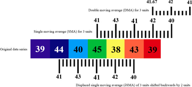
A time series can be defined as an ordered set of quantitative observations of a phenomenon recorded at successive regular periods [27]. Such time-series data can be mined for useful patterns suitable for various applications. A forecast of upcoming values in a time series is an application of similar nature. Because of the wide utility of forecasts [28] in domains from stock markets [29] to electrical machines [30], several methods for the analysis of time series data have been proposed to date [31], [32], [33], [34]. One such set of methods for forecasting future values in a time series is the moving average method [35], [36]. Now we will discuss some variants of the moving average technique to be utilized in our proposed approach (Fig. 4.) for analysis of the time series data of new Covid infections in different regions of the world.
Fig. 4.
Conceptual distinction of single (SMA), double (DMA) and displaced (MA) moving averages.
Definition 6 Simple Moving Average —
A Simple Moving Average (SMA) is the most commonly used variant of the moving average technique. It can be specified as the unweighted mean of previous k data points in a time series of n data entries. This implies that there are no weight factor values applied to any of the data points. In a series , , …, d of n data points, the mean of previous p points will be computed as given in Eq. (1) as follows:
(1) In this equation, p denotes the count of data points or subgroup size [37] used in computation, while represents the value of data point at period n. During each computation of values for succeeding data points, the new values will get added into the mean and the oldest ones will be dropped behind. This successive dropping and addition of values can be viewed as a moving transition of the SMA function through the time series (Fig. 4.). Hence, the technique is named as moving average. This successive computation of every next SMA for p points can be mathematically expressed in Eq. (2) as follows:
(2) In Eq. (2), we consider the sampling window of p points from to n+1 for calculating the next SMA of p points (). In this manner, the oldest value of is dropped and a new data point of value is added to the sum with the previous SMA ().
Definition 7 Double Moving Average —
In addition to the definition specified above, SMA is also defined as the single moving average. This definition means that the averaging has been performed only once by the SMA function over a set of observed data points in a time series. But in the double moving average (DMA) technique, the moving average values are computed twice [37]. Here, the first average is computed on the original data points of the time series , , …, d of n data points. The next moving average is computed on the resultant values of single moving averages , , …, sma of next m data points achieved in the previous step [38]. Hence, the double moving average, also known as dual moving average (DMA), can be considered as the moving average of SMA values. Computation of DMA from p number of precomputed SMA points has been presented in Eq. (3):
(3) As this form of moving average is computed from a precomputed result in 2 stages, the noise and fluctuations of original data are also more flattened or smoothed in it compared to SMA. This smoothed data, free from noise and fluctuations, is generally useful for the projection of underlying trends in a time series.
Definition 8 Displaced Moving Average —
It is the periodically displaced variant of the traditional moving average in either a backward or forward direction in a time series chart. No additional computation is required for the displaced moving average beyond the calculation of its classical variants discussed above. However, the average is simply shifted back or ahead of the data points by a specific window of periodic intervals.
A common usage of displaced moving averages is found in stock trading strategies [29] for better determination of market trends compared to usual moving averages [39]. The forward shift of moving average is termed as positive displacement and is presented by a rightwards movement of the values. Similarly, a negative displacement signifies a backward shift and is shown as a leftward transition of moving average values in the time series chart.
In the proposed work, we will be using a double moving average of 14 data points negatively displaced by an interval window of 14 units for projecting the current trend of the Covid-19 wave of new infections in a region.
3. Proposed work
In this section, we present our proposed approach with a detailed elaboration of components and process flow. We will first elaborate on the data utilized and later move towards the main work. But we initialize this section with the problem statement and the notations used.
3.1. Problem statement
Since its emergence, the count of new Covid infections has shown numerous spikes as well as drops in every region of the globe. These spikes and drops in the count have always created confusion about the future of this pandemic. This confusion has led to inconsistencies like underprepared infrastructure and lousy precautionary measures. Eventually, such inconsistencies have resulted into drastic waves of new Covid-19 infections. In this scenario, a well-defined demarcation of an uprise or downfall in a Covid-19 infection wave from temporary spikes or drops in the count is critically anticipated. Hence, we propose an approach for detecting marker points among these spikes and drops. These markers can enable us to forecast the behavior of an upcoming or ongoing wave of new infections with an observation window of minimum 7 days. Besides these markers, we also propose to project the upcoming count of new Covid infections for the next day with an average precision of more than 94% in a region.
3.2. Notations
As described earlier, our proposed model forecasts the rise and fall of a wave of Covid infections by detecting marker dates in the time series of infection counts. The model is composed of the following terms and notations:
| Actual infection count on day i | |
| v[C] | Range of new infection cases |
| Trend observation window (number of terms in one moving average for trend) | |
| Count observation window (number of terms in one moving average for count) | |
| w | Observation window (minimum number of days for which the count of new infections must increase) |
| Displacement gap | |
| M | Marker |
| Up-trigger | |
| Down-trigger | |
| s | Spike |
| d | Drop |
| Decimal base shift | |
| SMA | Corrected single moving average |
| DMA | Displaced double moving average |
3.3. Data description
The data utilized for the work proposed in this paper are obtained from the open-access resource of the ‘Our World in Data’ (OWID) repository [40]. OWID assembles and compiles the data from sources like the World Health Organization (WHO), Global Burden of Disease, World Bank, Johns Hopkins University, European Centre for Disease Prevention and Control (ECDC), and Blavatnik School of Government.
The data include and regularly update the date-wise confirmed counts of total infections, new infections, deaths, and vaccinations for 207 countries. To ensure geographic uniformity of data, our work employs the details of total and daily confirmed Covid-19 cases from 12 different countries, namely Argentina, Colombia, New Zealand, Australia, Cuba, Jamaica, Belgium, Croatia, Libya, Kenya, Iran and Myanmar. These details have been compiled into a time series database. The time series initiates from the date of a confirmed detection of the first case of Covid-19 infection in a region up to January 31, 2022. For example, the first confirmed case of Covid-19 infection in Argentina was detected on March 03, 2020, while the first infection in New Zealand was confirmed on February 28, and so forth. Hence, the respective time series of each country initializes on its own corresponding initializing date and extends to January 31, 2022.
Now, commencing with displaced DMA (DMA), we discuss the components of our proposed forecast models.
3.4. Displaced DMA (DMA)
For the time series data like a Covid wave, composed of several rises and falls in numbers, the determination of a trend can be challenging. To overcome this hardship, we employ displaced double moving average ( DMA), which forms the prime component of the proposed approach. We will be using it for tracking the trend of the Covid-19 infection wave by smoothing the time series data. DMA is a combination of double moving average (DMA) and displaced moving average ( MA) techniques. We implement this displaced double moving average ( DMA) function by a procedure ForecastTrend.
3.4.1. Derivation of DMA
To achieve the target DMA values, the computation of single moving averages (SMA) is essential. So, we first compute the SMA(14) of new infection counts throughout the time series for a trend observation window of 14 days as follows (Eq. (3)):
| (4) |
where:
(n) single moving average of next th period
actual infection count on day i
trend observation window or the number of terms in one moving average for trend
Similar to SMA(14), now we can derive the DMA(14) of infection counts over the precomputed SMA(14) values for the trend observation window of 14 periods given as:
| (5) |
where:
(n) double moving average of next th period
single moving average value on day k
trend observation window or the number of terms in one moving average for trend
Here, we can note the different counter variables i, j, and k for SMA and DMA, respectively. These variables are included to ensure the distinct range of periods for single and double moving average values in every iteration.
3.4.2. Displacement of DMA
The DMA(14) discussed above will generate a ‘smoothed out’ trend of new infection counts. However, these computed values of DMA will also appear ‘forward shifted’ in the time series chart by a gap equivalent to the subgroup size or observation window. This forward shift infers that each generated value of DMA(14) will appear 14 periods ahead of the corresponding actual count in the time series chart. Thus, we need to drag the computed averages backward with the same duration () of 14 periods to match the trend generated by DMA(14) values with the current count of new infections in the region. Therefore, we implement backward displacement () of DMA values by placing them number of points prior to their original positions given in Eq. (6) as follows:
| (6) |
This procedure provides us an output trend vector (T[D ]) comprising the difference of DMA(14) values computed over a trend observation window of () and displaced backward by a duration () to match the current infection count (Eq. (6)).
| (7) |
Throughout this section, we have denoted the number of terms or subgroup size [41] at each stage of the moving average as a trend observation window ().
We have selected 14 days as the value of this window () for the DMA. Similarly, the displacement gap () for a backward shift of the DMA values is also 14 days. The reason behind considering this duration for and parameters is that the maximum proposed incubation period for Covid-19 infections is 14 days [42]. Because of this incubation period, the medically advised isolation or quarantine period for Covid-19 patients is also 14 days [43]. Within this range of time, any significant change in the state of the infected population will be visible. This change will be projected in the form of a peak, decline, or sustaining of numbers.
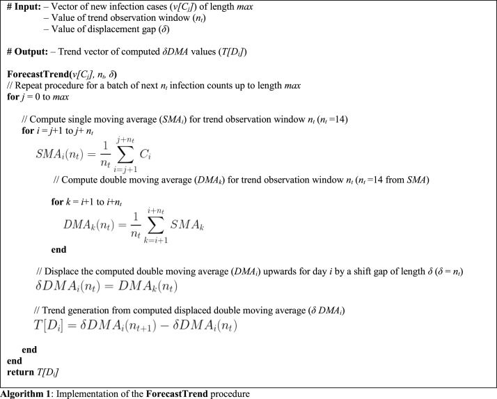
Hence, the procedure ForecastTrend generates the long-term trend (T[D ]) of the infection counts by implementing the displaced double moving average ( DMA) for a trend observation window of 14 days. A positive increment in this trend will project a rise in the Covid-19 wave, while a decrement will depict a fall. Now we present the algorithm (Algorithm 1) for implementing the ForecastTrend procedure.
3.5. Decimal base shift
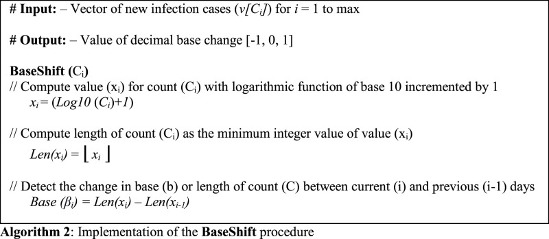
Detection of a marker date against a trend is our next target in the proposed approach. The marker must be robust enough to satisfy a conditional limit upon the count of newly infected population for a predefined timespan. Here, we will be utilizing the shift in decimal base () of infection counts as the proposed marker. By the term decimal base, we infer the number of digits present in a value. So, any difference or shift in the decimal base of new infection counts with a rising or dropping DMA will be considered as a marker which includes up-trigger (), down-trigger (), spike (s), and drop (d). To compute this shift, we first need to retrieve the decimal base from the value of current infection count and then compute its difference from its predecessor value on the previous day. This section discusses the implementation of this shift () in the decimal base of infection counts as the BaseShift procedure.
3.5.1. Length of infection counts
As the infection counts are integer values represented in decimal form, so for retrieving their decimal base, we compute their logarithm in base 10. The value of an integer i composed of n digits lies between 10 and 10. This implies that log10(n) will fall between (n – 1) and n inclusive of both. Further, an addition of 1 to this value will provide the number () of digits as follows:
The achieved value () will be in decimal format with a fractional component attached to its integer part. Therefore, we will now apply the floor function to cut down the fractional part, retrieving the actual length (n) as a result. Mathematically, this function is expressed as:
3.5.2. Shift in count length
After retrieving the length of the current infection count (Len(x )), we now need to detect any change in its decimal base from its previous values. Thus, this change or shift of base is computed as the difference of the current count length (Len(x )) and its adjacent predecessor (Len(x )) given as:
This approach has been presented in algorithmic format in Algorithm 2.
Now we elaborate our approach with an example. For the region of Australia, 75 new infections were witnessed on March 17, 2020. However, a count of 116 was observed on the next day, that is, on March 18, 2020. Now the logarithm of base 10 for 75 results into 1.87506. An addition of 1 to this number will provide 2.87506. In this number, the integer component is equivalent to the number of digits in 75, i.e., 2. However, the fractional component is no longer required and is hence truncated by the floor function. The final result will be 2.
Similarly, the value of logarithm of base 10 for 116 with an addition of 1 will be 3.06445, which, post truncation, will provide an integer value of 3. We will further compute the difference between the current and previous lengths to detect the change in count lengths. Here, a positive shift in base of 1 unit from 2 to 3 is visible between these 2 dates, which can possibly represent an up-trigger () or a spike (s). Similarly, a negative shift can depict a down-trigger () or a drop (d).
3.6. Corrected SMA (SMA)
Forecasting the upcoming count of new infections in a region with high precision is a critical issue. This issue remains decisive in medical preparations and infrastructure buildup to combat the pandemic. To address this issue, the next goal of our proposed approach is to devise a novel variant of the moving average technique for generating the upcoming infection count for the next day with minimum error. We know that, generally, a gap always exists between the forecasted and actual values for every forecasting technique. This gap, termed as ‘error,’ forms the basis of various performance metrics for a forecast model like mean bias error (MBE), mean average error (MAE), mean square error (MSE), root mean square error (RMSE), and more.
We propose to utilize this gap to improve the efficiency of the moving average. Thus, we add the average of the errors attained at a stage of moving average to the value of the next stage. This addition can be considered as a form of ‘correction’ of moving average, hence named the ‘corrected moving average ( MA)’ method. This proposed correction aims to update the mean of a set of values with the average of the set of corresponding errors. Here, the average function evenly distributes any fluctuation in errors of the set, similar to as it does for the set of original values.
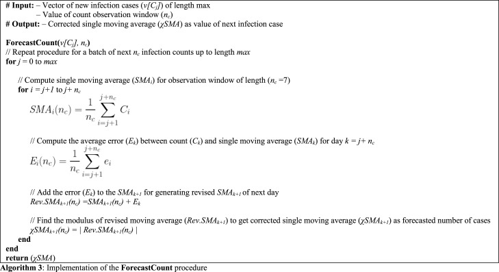
In this section, we will implement this approach on the single moving average (SMA) as the ForecastCount procedure (Algorithm 3), formulating the corrected single moving average (SMA) for forecasting upcoming infection counts. The proposed approach accepts the vector of new infection counts (v[C]) and the value of count observation window () is set to 7 days for processing. Here, denotes the number of values at a single stage of SMA similar to the trend observation window () of the DMA model discussed in Section 3.4. However, the value of count observation window () is accepted as half of the trend observation window () to match the minimum incubation period for Covid-19 [42]. Here, can be considered as the lower timeline limit of the incubation period to spot any changes in the state of the infected population. The proposed approach proceeds as follows:
3.6.1. SMA computation
In the first step of this method (Eq. (8)), we compute the SMA using the classical moving average technique by accepting 7 values () at every stage. This computation proceeds for the whole range or vector of new infection cases (v[C ]). From this step, we will achieve the forecasted values of infections.
| (8) |
3.6.2. Error determination
As discussed above, an error is expected to exist between the forecasted and actual values of infection counts. Thus, at this step, we compute the error () between count () and the single moving average value () for day k as:
| (9) |
3.6.3. Average error
Now we compute the average of errors () retrieved for the number of stages at stage i as:
| (10) |
3.6.4. SMA correction
This step performs the main component of the proposed approach by adding up the error () attained at stage k to the moving average of stage k+1 () to generate a revised SMA (Rev.SMA ) for the next day.
| (11) |
3.6.5. Absolute revised SMA
Finally, we compute the modulus of the revised moving average (Rev.SMA ) to achieve the corrected single moving average ( ) as the forecasted number of cases.
| (12) |
It should be noted that the addition of average error () to the next stage of SMA can also generate a negative value. However, the number of projected new infections cannot be negative in any case. Thus, this step is crucial for neutralizing any negative value of .
3.7. Decision rules generation
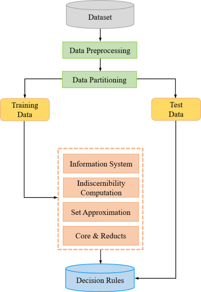
As discussed in Section 2.1 above, the detection of markers depicting any rise or fall in the trend of Covid-19 infections needs a guiding or filtering mechanism. This filter is provided by the decision rules generated from the provided Covid-19 database through the use of rough set theory. In this section, we will discuss the process of generation of these rules (Fig. 5). As discussed earlier, the rough set decision rules for any process are composed of conditional features P {P 1, , , … P and a decision feature D in the following format:
Thus, the generation of decision rules is a process that requires the selection of appropriate variables from the information system. To set up the information system table from the provided Covid-19 database, we select the date and count of new infections () for every country under consideration.
Fig. 5.
Flowchart of decision rule generation process by use of rough sets.
1. Preprocessing
We now execute the ForecastTrend procedure to execute DMA(14) over the new infections () and generate the trend (T[D ]). The trend will help in estimating the direction of the Covid-19 wave. Here, a positive value of T[D] will project a rise in wave while the negative ones will present a fall. We also execute the BaseShift procedure to derive the decimal base shift () variable. Execution of these procedures can be considered under the preprocessing stage. This preprocessing sets the trend (T[D]) and base shift () as conditional features, while the marker (M) can be stated as the decision variable.
2. Data partitioning
We now partition our database into a 70:30 ratio of training and testing datasets for the 12 countries. As the count of infection dates differs for each country, the numbers of records in their training and testing datasets also differ.
3. Model generation
Now we compute the indiscernibility of attributes from the information system composed of the training dataset. We further calculate the set approximations to discard the conflicting records of the boundary region. The approximations lead us to discover the core and reduct attributes by estimating their dispensability. By utilizing the core and reduct attributes, we will mine the decision rules.
4. Validation
For a minimum observation window of 7 days, the decision rules are further validated against the records of the testing dataset with an accuracy of 96.4%. For trend value (T[D]), base shift (), and observation window (w), the rules for marker (M) are as follows:
| (13) |
| (14) |
| (15) |
| (16) |
| (17) |
| (18) |
| (19) |
5. Decision filter
This rule base is implemented as a decision filter for the detection of markers by the ForecastMarker procedure. The rules can be summarized in the following manner. For the first positive base change ( ) observed over a positive trend (T[D]) after an observation window of at least 7 days, an up-trigger () will be marked. But all upcoming similar positive base changes observed after a will be recorded as spikes (s). Similarly, the negative base shifts ( ) observed over negative trends (T[D]) after at least 7 days will be considered as down-trigger () or drops (d). No marker will be considered if the decimal base does not change for a positive or negative trend. However, this condition does not imply the absence of a rising or deprecating infection wave.
4. Methodology
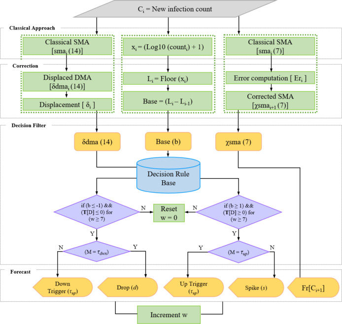
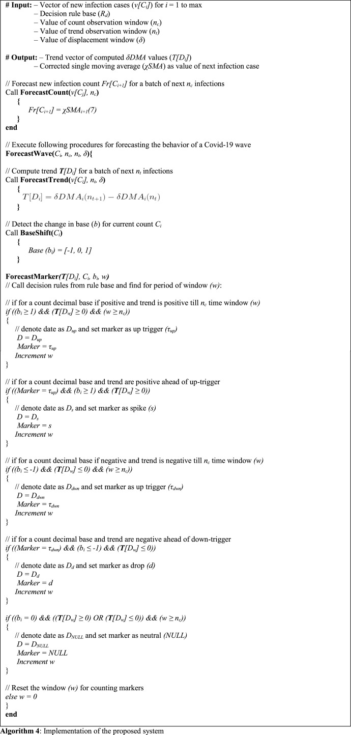
As discussed earlier, this approach is composed of moving average components and is directed by rules of rough set theory. So, in this section, we will discuss the methodology of implementing these components as an integrated assembly (Fig. 6.). This assembly is also presented in the algorithmic format in Algorithm 4. It receives the range of new infection cases (v[C ]), count observation window (), trend observation window (), and displacement window () as input.
Fig. 6.
Architecture of the proposed approach.
4.1. System implementation
In the first step, the projected value of the new infection count for the upcoming day is forecasted by calling the ForecastCount procedure. This procedure executes SMA function for a count observation window () of 7 days and generates an estimate of new infections for the next day. Further, a combination of DMA and base shift is used for detecting spikes (s), drops (d), up-triggers (), and down-triggers () by the procedure ForecastWave.
This procedure first determines a positive or negative trend of the Covid-19 infection wave by calling the ForecastTrend sub-procedure. Here, ForecastTrend returns a vector of T[D] values as the trend for a provided range of infection counts. Further, the BaseShift sub-procedure detects changes in the decimal base of the infection counts. After determining the trend and base shift, the ForecastMarker procedure executes the decision rules discovered by the rough set theory over the available Covid-19 database. For a provided observation window (w 7), it classifies the −1, 0, and 1 values of BaseShift into markers as spikes (s), drops (d), up-triggers (), and down-triggers ().
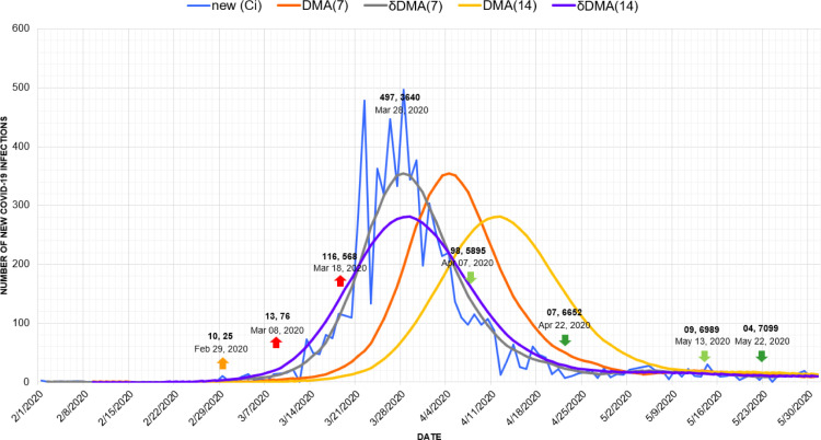
Here, after passing the duration of the observation window of 7 days in a positive trend (T[D]) of infections, the very first point of any significant increase in count marked by the decimal base shift is termed as the first up-trigger () depicted by an upward orange arrow (Fig. 7). The upcoming points of increase following can be regarded as spikes (s) shown by upward red arrows. Here, indicates the start of a Covid-19 wave while the spikes (s) forecast a further rise in an ongoing wave. In Fig. 7, the rise in wave forecasted by up-trigger and spike on February 29 and March 08, respectively attain the peak infection count of 497 cases on March 28. Similarly, with a negative T[D], the first point of decrease in infections marked by a decimal shift is termed as a down-trigger () displayed by a light green downward arrow. Also, further declines in counts are projected by drop (d) markers exhibited by downward dark green arrows. The fall of wave projected by the down trigger on April 07 leads to a further drop on April 22 to mere 07 cases. An up-trigger can be followed by multiple spikes displaying the increase in infection counts throughout the expansion period of an upward wave (Fig. 2). Similarly, several drops can follow a down-trigger representing the de-escalation of the wave. It must be noted that the direction of infection trend (T[D]) must favor the sign of BaseShift to be considered a marker. It implies that only a positive base shift observed after a positively increasing trend of minimum 7 days will be considered an up-trigger () or a spike (s). A similar combination of a negative base with a negative trend will be stated as a down-trigger () or a drop (d). However, a negative base shift parallel to a positive trend or vice-versa will not be considered the same as above.
Fig. 7.
Interpretation of the first Covid-19 wave in Australia.
4.2. Case study: First wave of Covid-19 infections in Australia
For further elaboration of our methodology, here we will discuss its implementation with the case study of the first Covid-19 wave in Australia [44].
In Fig. 7, we presented the details of various marker points consisting of up and down triggers, spikes, and drops in the first Covid-19 wave scenario in Australia. This scenario is further elaborated in the time series graph presented in Fig. 8. The graph depicts a series of different dates with changing new infection counts (). Besides the new infection counts () presented by the blue line, 4 other lines are also present in the graph. These lines illustrate the trends computed from through different moving average techniques. The orange and yellow lines present the trends of new infections retrieved by the DMA(7) and DMA(14) models. It must be noted that both of these lines are shifted ahead of , which indicates the gaps between the real counts and the trends forecasted by these models. Similarly, the gray and violet lines running along with the infection count present the trends computed by DMA(7) and DMA(14) techniques. The trends are displaced backward by a displacement window of 7 and 14 days. These displacements place the respective trends to match the actual counts, making them more relevant and valuable.
Fig. 8.
Timeline graph of first wave of new Covid-19 infection cases in Australia.
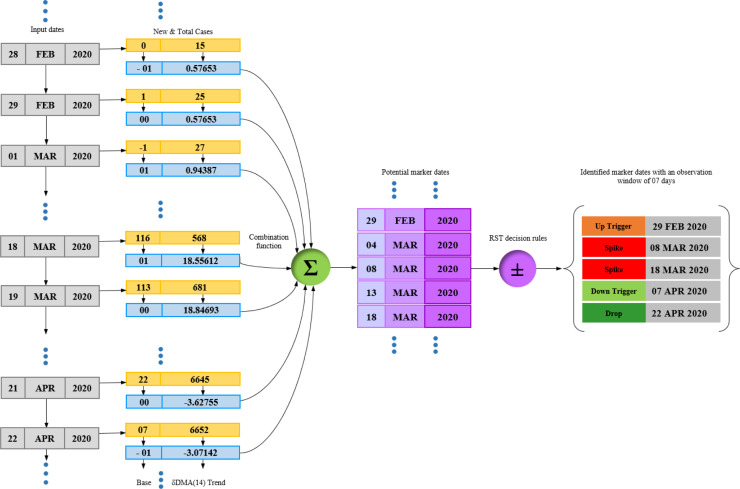
Now we elaborate the generation of markers against the trend of DMA(14) as presented in Fig. 9.
Fig. 9.
Flowchart of marker detection from DMA(14) trend of a Covid-19 wave.
The first visible count of 04 infections was detected in Australia on January 26, 2020, with a decimal base range of 01. The function of our proposed approach retrieved the positive trend (T[D]) of value 0.0357 for the upcoming wave that started from February 17, 2020. Parallel to this positive trend, after crossing the count observation window of 7 days, the BaseShift procedure detected an up-trigger () of 10 new infections on February 29 against a trend value of 0.5765. This up-trigger confirmed the start of the first Covid-19 wave in Australia. The next shift in decimal base with 13 new cases was spotted on March 08 as the forecast of the first spike of the upcoming wave. It was succeeded by another shift to the next decimal base range of 2 and recorded as another spike with an increase of counts from 75 to 116 on March 18, 2020. Similarly, the start of a negative trend in this Covid wave was depicted by the function on March 30 for 377 new cases with a reducing trend (T[D]) of −3.7092. After passing the observation window of 7 days, the earliest negative shift from a decimal base of 3 to 2 was recorded as the first down-trigger () on April 7 with 98 infections against a trend value of −16.4031. This down-trigger was followed by a drop (d) of 7 more new infections on April 22, confirming the fall of the first Covid wave.
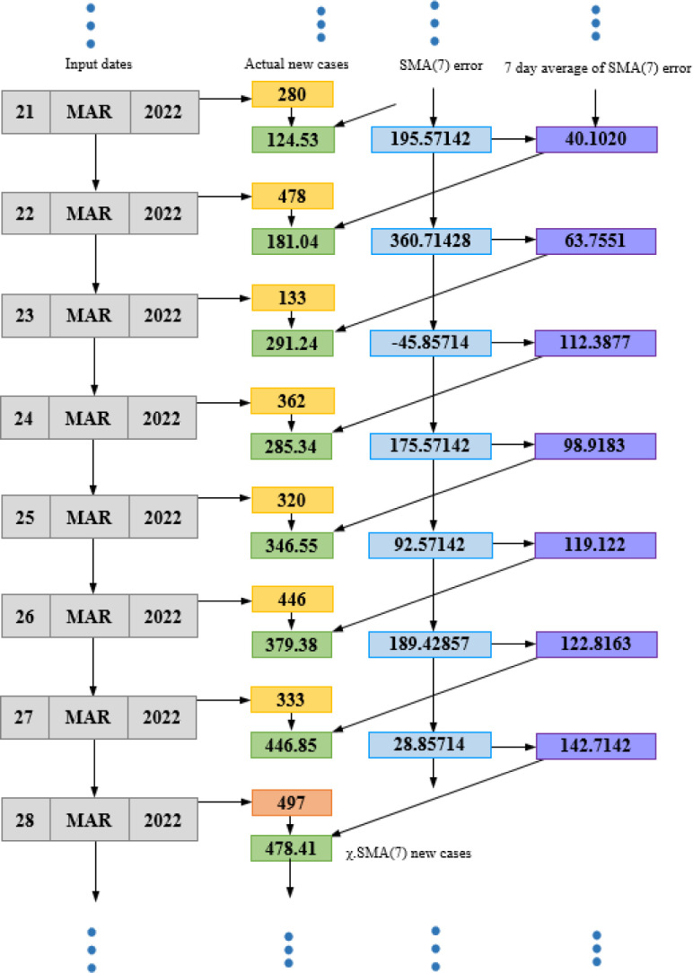
Regarding the forecast of the upcoming count of cases for the next day (Fig. 10), with respect to the actual 1701 witnessed on December 01, 2021, the function projected an approximate count of 1410 upcoming infections. Compared to the results of the baseline techniques of SMA(7) as 1362 with an error percentage of 19.926%, and DMA(7) as 1364 with an error percentage of 19.85%, the forecasted with the lowest error of 17.139%. In terms of average mean bias error also, the performed the best with the lowest average error of 0.0389 compared to the average error of 7.785 of SMA(7) and 16.147 of DMA(7) baseline techniques.
Fig. 10.
Computation of upcoming infection count by SMA(7) function.
5. Experimental results
In this section, we will confer on the experimental details and results of the proposed approaches. But we will initiate this section with the performance measures that will be used to evaluate the efficiency of these approaches.
5.1. Performance measures
In our proposed work, the DMA(14)-base shift approach forecasts the behavior of the Covid-19 wave while the SMA(7) technique is focused on forecasting upcoming infection counts. Thus, we will be considering 2 distinct classes of performance indicators for evaluating the performances of the 2 proposed models. We commence this section with an elaboration of bias-based indicators.
Bias indicators: The mean bias error (MBE) and normalized mean bias error (NMBE) are the bias-based indicators to be used for the performance evaluation of the DMA(14)-base shift model. These indicators are based on the average error present in the values. This implies that strong chances persist of cancellation of positive and negative errors. This property of MBE is considered a major limitation that restricts its usage. However, we will be utilizing it here to measure the performance of the models.
5.1.1. Mean bias error (MBE)
The difference between the actual () and the forecasted () value is termed as mean bias error (MBE). With n number of values or points, MBE can be mathematically stated as (Eq. (20)):
| (20) |
5.1.2. Normalized mean bias error (NMBE)
It is a normalization of the MBE indicator, which makes the results of MBE comparable by scaling them. NMBE computes the global difference between actual and projected values by quantifying the MBE through its division by the average of projected values (Eq. (21)).
| (21) |
Metrics like mean absolute error (MAE) and mean square error (MSE) defer the sign of errors to record the positive as well as negative errors also as positive quantities. This deferment of sign or direction, in turn, practically increases the final positive error manifolds and abandons the negative displacements altogether, losing the direction of the trend underlying the data.
Contrarily, MBE treats each error with its original positive or negative sign. Due to this property, strong chances of cancellation among positive and negative errors persist. This property of MBE is considered a major limitation that restricts its usage. However, in the case of the DMA models, our purpose is to project the trend visible in the time series data rather than forecasting the quantities with exactness. As MBE and NMBE are interrelated, we will be using both for the performance measurement of our DMA models.
We now proceed towards the description of precision-based performance indicators.
Precision indicators: Indicators based on precision specify the spread of the gap between the actual and forecasted values. But instead of positive or negative directions, these indicators measure only the magnitude of errors present in data. Here, the performance of the proposed SMA model will be evaluated by four different parameters [45], namely mean absolute error (MAE), mean square error (MSE), root mean square error (RMSE), and mean absolute percentage error (MAPE).
5.1.3. Mean absolute error (MAE)
The MAE measures the average magnitude of the errors in a set of forecasts without considering their positive or negative directions. This implies that the MAE is the average of the absolute values of the differences between forecast and the actual observation (Eq. (22)). The MAE can also be considered as a linear score which infers that all the distinct differences are equally weighted in the average.
| (22) |
5.1.4. Mean square error (MSE)
The average of squared differences between actual and forecasted values is computed by mean square error. In terms of regression, MSE states the proximity of a regression line to a set of error points. This proximity is calculated as the distances of error points relative to the regression line and squaring them removes any negative signs. Mathematically, MSE is stated as (Eq. (23)):
| (23) |
5.1.5. Root mean squared error (RMSE)
RMSE can be considered as a quadratic score that measures the average magnitude of the error. Technically, it is defined as the square root of the squared difference among the forecasted () and observed () values of a quantity (Eq. (24)). Here, the squaring of errors before computation of their average allocates higher weights to large errors, thus projecting them distinctively. RMSE can be used in combination with MAE to detect the variations in errors among a set of forecasted values.
| (24) |
5.1.6. Mean absolute percentage error (MAPE)
The mean absolute percentage error (MAPE) can be stated as the average of the absolute percentage errors of forecasts. Here, the percentage errors are totaled without considering their positive or negative signs.
| (25) |
In the next section, we will conduct an empirical analysis of the results of our proposed approaches over the Covid-19 time series database of 12 countries.
5.2. Empirical analysis
As discussed earlier, in this paper, we have analyzed the pandemic time series of 12 countries from their initial dates to January 31, 2022. Thus, in this section, we will inspect the results of the proposed work.
We constructed the SMA(7) model based on the single moving average (SMA) technique. The SMA(7) model forecasts the upcoming count of new Covid infections by computing the average of the infection counts for the previous 7 days. Its accuracy was improved by adding the average of residual errors derived as differences between actual and forecasted counts for an observation window of 7 days. This improvement fitted the SMA(7) model to the actual infection count with an average mean absolute deviation (MAD) of 787.61 compared to 859.66 for classical SMA(7) and 1081.369 as MAD for SMA(14). As the MAD of SMA(7) model is reduced significantly against the baseline models, consequently, the mean square error (MSE) and root mean square error (RMSE) are also reduced in a similar proportion. The minimum mean absolute percentage error (MAPE) of value 12.63 has been recorded for Iran by SMA(7) compared to 14.43 by SMA(7) and 19.33 for SMA(14) models, respectively. Likewise, the second minimum MAPE of value 16.10 was recorded by SMA(7) for Colombia against a MAPE of 17.48 by SMA(7) and 23.05 for SMA(14) models. In Table 2, we have compared the forecast errors as MAD, MSE, RMSE, and MAPE values generated by the 3 techniques over the time series data of new Covid-19 infections recorded in 12 countries.
Table 2.
Comparison of average forecast errors of SMA(7), SMA(7) and SMA(14).
| COUNT |
SMA(7) |
SMA(7) |
SMA(14) |
|||||||||
|---|---|---|---|---|---|---|---|---|---|---|---|---|
| MAD | MSE | RMSE | MAPE | MAD | MSE | RMSE | MAPE | MAD | MSE | RMSE | MAPE | |
| Argentina | 2630.207 | 36280918.6 | 6023.364 | 26.822 | 2923.695 | 51639878.73 | 7186.089 | 27.831 | 3542.809 | 90277202.18 | 9501.431 | 31.923 |
| Colombia | 1115.276 | 3535904.72 | 1880.4 | 16.101 | 1278.581 | 4750336.665 | 2179.526 | 17.481 | 1815.097 | 9327479.961 | 3054.092 | 23.059 |
| New Zealand | 7.763 | 242.763 | 15.580 | 52.886 | 8.016 | 256.757 | 16.023 | 47.894 | 9.863 | 371.085 | 19.263 | 54.054 |
| Australia | 1028.707 | 30953185.7 | 5563.558 | 38.786 | 1135.249 | 38333129.71 | 6191.375 | 42.693 | 1635.512 | 71543610.97 | 8458.345 | 55.774 |
| Cuba | 158.293 | 143672.781 | 379.041 | 29.089 | 195.420 | 189905.285 | 435.781 | 31.876 | 301.575 | 399625.924 | 632.159 | 40.823 |
| Jamaica | 57.252 | 13396.590 | 115.743 | 48.149 | 58.377 | 14744.85052 | 121.428 | 47.994 | 71.753 | 23214.111 | 152.361 | 54.938 |
| Belgium | 2455.838 | 54780112.8 | 7401.358 | 32.395 | 2489.568 | 53461698.4 | 7311.750 | 35.924 | 2734.681 | 57821300.81 | 7604.0318 | 44.334 |
| Croatia | 448.492 | 883089.751 | 939.728 | 71.769 | 473.069 | 888331.954 | 942.513 | 75.480 | 526.712 | 1032634.766 | 1016.186 | 85.496 |
| Libya | 229.245 | 208876.011 | 457.029 | 23.358 | 229.950 | 205674.495 | 453.513 | 21.547 | 248.930 | 237257.647 | 487.091 | 23.520 |
| Kenya | 149.255 | 71222.956 | 266.876 | 48.648 | 158.799 | 78814.079 | 280.738 | 51.013 | 190.701 | 120544.741 | 347.195 | 59.800 |
| Iran | 1055.076 | 4128910.12 | 2031.972 | 12.630 | 1230.285 | 5209738.468 | 2282.485 | 14.433 | 1702.150 | 8718068.397 | 2952.637 | 19.333 |
| Myanmar | 115.942 | 59437.671 | 243.798 | 39.250 | 135.022 | 84260.919 | 290.277 | 36.824 | 196.640 | 174582.349 | 417.830 | 45.320 |
| 787.612 | 10921580.9 | 2109.871 | 36.657 | 859.669 | 12904730.86 | 2307.625 | 37.583 | 1081.369 | 19972991.08 | 2886.885 | 44.865 | |
We have further analyzed the count forecast performance of the proposed SMA(7) model against other baseline techniques. It should be noted that this projection can change with any upcoming count of new infections. Similar to the average forecast performance presented in Table 2, SMA(7) also outperforms its baseline counterparts in terms of daily count forecasts (Table 3). Here, SMA(7) resulted in a minimum average forecast error of 61% compared to 99.81% of SMA(7) and 137.49% of SMA(14). The best forecast of daily infection count (47.93) recorded for January 31, 2022, was projected by SMA(7) for Kenya with an error of only 4.21% against the actual count of 46 infections. In this case, SMA(7) presents significant improvements against errors of 243.47% by SMA(7) and 474.68% by SMA(14) models. In terms of a worst-case scenario of Croatia, the errors of 479.95% by SMA(7) and 484.68% by SMA(14) are still inferior to a lower error of 460.46% projected by SMA(7).
Table 3.
Comparison of daily forecast errors of SMA(7), SMA(7) and SMA(14) recorded on January 31, 2022.
| ERROR | COUNT on 31–01–2022 |
SMA(7) |
SMA(7) |
SMA(14) |
||||||
|---|---|---|---|---|---|---|---|---|---|---|
| For Count | For-Error | % For-Error | For Count | For-Error | % For-Error | For Count | For-Error | % For-Error | ||
| Argentina | 43472 | 40202.979 | 3269.020 | 7.519 | 67521.142 | 24049.142 | 55.320 | 88594.214 | 45122.214 | 103.796 |
| Colombia | 15284 | 13115.142 | 2168.857 | 14.190 | 18828.285 | 3544.285 | 23.189 | 23441.5 | 8157.5 | 53.372 |
| New Zealand | 204 | 144.122 | 59.877 | 29.351 | 113 | 91 | 44.607 | 92.071 | 111.928 | 54.866 |
| Australia | 36719 | 51888.326 | 15169.326 | 41.311 | 54019.714 | 17300.714 | 47.116 | 58659.642 | 21940.643 | 59.752 |
| Cuba | 2119 | 2692 | 731.591 | 34.525 | 2937 | 915 | 43.180 | 3105.571 | 1038.928 | 49.029 |
| Jamaica | 410 | 437.326 | 27.326 | 6.665 | 648.142 | 238.142 | 58.083 | 848.857 | 438.857 | 107.038 |
| Belgium | 99314 | 52759.040 | 46554.959 | 46.876 | 51240.857 | 48073.142 | 48.405 | 46085.285 | 53228.714 | 53.596 |
| Croatia | 1445 | 8098.775 | 6653.775 | 460.468 | 8380.285 | 6935.286 | 479.950 | 8449.071 | 7004.071 | 484.710 |
| Libya | 4429 | 3819.346 | 609.653 | 13.765 | 2830.286 | 1598.715 | 36.096 | 1994.142 | 2434.857 | 54.975 |
| Kenya | 46 | 47.938 | 1.938 | 4.214 | 158 | 112 | 243.478 | 264.357 | 218.357 | 474.689 |
| Iran | 28995 | 19559.571 | 9435.428 | 32.541 | 13384.142 | 15610.857 | 53.839 | 8796.142 | 20198.857 | 69.663 |
| Myanmar | 278 | 197.755 | 80.244 | 40.577 | 169 | 109 | 64.497 | 150.714 | 127.285 | 84.454 |
| 61.00074 | 99.813887 | 137.4955 | ||||||||
Now we evaluate the performance of the second proposed model of DMA(14) that projects the trend of Covid-19 infection waves. We will use mean bias error (MBE) to estimate the gap between the projected trend and the actual time series. Here, the trendline projected by the DMA(14) model fits nearest to the wave of infection counts (Table 4). This is depicted by the minimum MBE of 34.75 compared to MBE of 205.67 by DMA(7) and 439.68 by DMA(14) model. As a consequent indicator of MBE, the NMBE of DMA(14) also attains a minimum value of −3.356 against the 29.74 (DMA(7)) and 66.95 (DMA(14)) values. However, a negative NMBE represents that the trend of the proposed model is smaller than the original trend line.
It must be noted that the length of the displacement window among these models differs by a duration of 7 days. DMA(7) starts after 14 days, while DMA(7) initiates after 7 days of its parent SMA computation. This implies that DMA(7) has been shifted upward or backward in time series by a displacement of 7 units to match the wave of actual numbers. Similarly, DMA(14) starts without any backward displacement after 28 days. On starting with a displacement window of 14 units, this DMA(14) is portrayed as the DMA(14). The accuracy of this displacement is crucial to match the projections against the actual counts.
Table 4.
Comparison of trend projection performance by DMA(7), DMA(14) and DMA(14).
| TREND |
DMA (7) |
DMA(14) |
DMA(14) |
|||
|---|---|---|---|---|---|---|
| MBE | NMBE | MBE | NMBE | MBE | NMBE | |
| Argentina | 772.1430356 | 19.54561898 | 1896.15562 | 33.58767343 | 139.3565127 | −0.861120052 |
| Colombia | 229.2168405 | 15.30654897 | 527.1117111 | 26.60781529 | 51.56612062 | −0.643813643 |
| New Zealand | 1.42425318 | 47.41597051 | 1.769185485 | 71.09265313 | 0.035457674 | −7.441309463 |
| Australia | 590.8276047 | 31.89637674 | 1383.89143 | 113.5424323 | 225.6506074 | −6.501396027 |
| Cuba | 34.05127664 | 20.29351115 | 67.87499615 | 36.76918559 | 4.690984086 | −2.555473299 |
| Jamaica | 7.452019746 | 22.03676335 | 19.70685548 | 40.25481513 | 3.092397652 | −2.574716535 |
| Belgium | 540.4560967 | 84.31176625 | 952.7358309 | 259.4170419 | −6.12845481 | −4.276487513 |
| Croatia | 90.8856495 | 36.17748388 | 175.7354829 | 70.3852792 | 1.903376815 | −4.753484139 |
| Libya | 34.3157281 | 28.42878751 | 47.0839368 | 52.09404609 | −1.42451174 | −3.288684683 |
| Kenya | 1.851074749 | 17.10181175 | 7.27152568 | 37.23975243 | 2.179380665 | −2.403374823 |
| Iran | 163.2725468 | 10.07760268 | 193.2607404 | 13.71961639 | −4.03123045 | −0.838485678 |
| Myanmar | 2.151119058 | 24.39752169 | 3.576310154 | 48.72693533 | 0.226001512 | −4.1398242 |
| 205.6706038 | 29.74914696 | 439.6811354 | 66.95310385 | 34.75972018 | −3.356514171 | |
6. Discussions
This section will discuss various aspects and challenges met in this manuscript and their plausible answers in terms of component techniques, functional specifics, and results.
6.1. Comparative analysis
Continuing from the results of the previous section, here we present a comparison of the various approaches on Covid-19 forecast (Table 5). We also compare our proposed approach against these approaches. We can broadly categorize the works discussed in this manuscript into ARIMA-based and Compartment-based approaches. As the name suggests, the ARIMA technique comprises the major algorithmic component of the ARIMA-based approaches [10], [11]. On the other hand, every compartment-based approach partitions the population of the region under consideration into compartments like susceptible (S), infected (I), recovered (R), and dead (D) populations for the generation of models [13], [14], [15], hence the name.
Table 5.
Comparative summary of selective works on Covid-19 forecast.
| Reference | Year | Data | Constituent technique | Proposed work | Advantages | Limitations |
|---|---|---|---|---|---|---|
| ARIMA-based approaches | ||||||
| [10] | 2020 | Italy, Spain, Turkey | Auto Regressive Integrated Moving Average (ARIMA), autocorrelation function (ACF), partial autocorrelation (PACF) | Predicting the number of cases and deaths from time series data. |
Month-wise forecast of infection and death counts. |
1. Complex selection of p,q,r parameter values for appropriate ARIMA model. 2. Counts saturate after a threshold time. |
| [11] | 2020 | India, Brazil, Spain, Russia, United States | Auto Regressive Integrated Moving Average (ARIMA), Hannan and Rissanen algorithms. | Predicting the number of cases and deaths from time series data. |
Count-wise and month- wise forecast of infection cases. |
1. Complex selection of p,q,r parameter values for appropriate ARIMA model. 2. Counts saturate after a threshold time. |
| Model-based approaches | ||||||
| [12] | 2020 | United States, Slovenia, Iran, Germany | Simple iteration of infection counts for a specified number of days |
Determination of the average growth rate of infection from daily values of confirmed cases. |
Simple implementation | 1. Based on infection growth rate. 2. Provision for only first insights of the pandemic 3. Accuracy is not assured |
| Compartment-based approaches | ||||||
| [13] | 2020 | China, Italy, France | Differential evolution algorithm implemented on mean-field kinetics of the epidemic spread. |
Modeling of susceptible (S), infected (I), recovered (R), dead (D) population counts. |
1. Model captures gross features of the outbreak. 2. Simple implementation |
1. Assumes that counter measures must cause a quick and effective reduction in infection rate. 2. Counts saturate after a threshold time. |
| [14] | 2020 | China | Linear regression modeling |
Estimations of the basic reproduction number (R0) and the per day infection mortality and recovery rates on the basis of SIDR model. |
Flexible and elaborate implementation | Assumption of the count of infected and recovered populations to be 20 and 40 times respectively, relative to the actual counts, leading to possible gaps in results. |
| [15] | 2020 | India | Nonlinear differential equation modeling | Modeling of susceptible (S), asymptomatic (A), recovered (R), infected (I), isolated infected (I), and quarantined susceptible (S) population counts. |
1. Model captures multiple features of the outbreak. 2. Simple implementation |
1. Dependent on a predefined set of parameters. 2. Lacks sensitivity to change in infection counts. |
Another category under which Covid-19 forecast applications can be placed, is the category of model-based approaches. These approaches comprise logical or mathematical models for structuring the forecast on the basis of population counts [12]. We place our proposed approach under this category. The forecasts on the rise and fall of the waves of infection counts form the primary component of our approach, which is not addressed by any other work. These forecasts on the behavior of infection waves form the major distinction of our proposed work from the approaches discussed here. Apart from simple implementation, the execution of our approach is also independent of any dynamic parameter, such as infection or recovery rates. Hence, in broad terms, it can be employed for modeling any epidemic over any specified geographic profile and population. Further, we have implemented our approach on an extensive range of population counts from 12 different countries. Also, the discussed approaches forecast on the upcoming waves up to the accuracy of months for a provided region. Contrarily, our proposed model is capable of forecasting the behavior of an infection wave with a sensitivity of 7 days. Similarly, it also forecasts the upcoming counts of new infections under a minimum observation window of 7 days with high accuracy.
6.2. Results per country
As described earlier, including the case study of the first Covid-19 wave in Australia, we have analyzed the Covid-19 infection data of 12 countries. Hence, here we will confer upon the results achieved by implementing the proposed approach over the data of these countries.
The prime observation of these countries is that the infection counts due to the Omicron variant of Coronavirus have surpassed all the previous numbers. The wave caused by Omicron variant has led to the suppression of preceding waves in the time series graphs of these countries. Now we will elaborate on the individual observations for each country along with their time series graphs in this section.
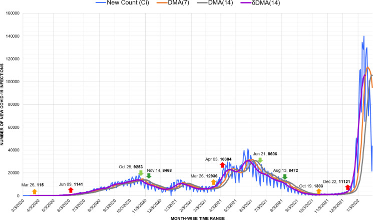
In South America, Argentina depicts a perceptible rise and fall of 3 waves (Fig. 11). However, due to the local spikes and drops, the fall of the first wave was not marked evidently, and the second wave initiated from it on March 26, 2021, with 12,936 new infections. Here, considering that the major number of infection cases was imported, decisions like closing borders, establishing quarantine, and canceling flights helped Argentina to sustain better during the first wave [46].
Fig. 11.
Timeline graph of new Covid-19 infection cases in Argentina.
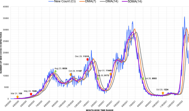
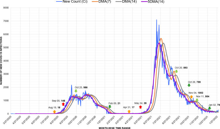
On the other hand, Colombia is among the worst-hit South American nations by Coronavirus. Here, the markers of our proposed approach have detected the explicit behavior of each wave. Surprisingly, the third wave, marked from April to September 2021, was undeniably as devastating as the fourth wave (Fig. 12.). Improper timing of pandemic responses like vaccination and instituting unpredictably long lockdowns have been plausible reasons for the distressing state of the pandemic in Colombia [47]. Nevertheless, similar to Argentina, the second wave initiated from the minor drop of the first wave on October 29, 2020, with 11,187 new infections.
Fig. 12.
Timeline graph of new Covid-19 infection cases in Colombia.
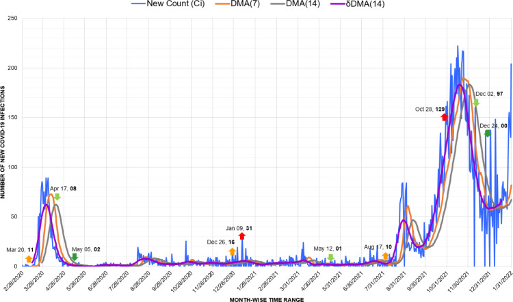
In the region of Oceania, New Zealand managed to control the pandemic successfully after the first wave marked from March to May 2020. In addition to measures like adequate testing, timely procurement of medical supplies, closure of schools, sealing of borders, and social distancing made a positive impact. Here, a 4-level risk assessment system helped the New Zealand administration significantly to respond to the pandemic in a strong and efficient manner [48]. The system facilitated suitable categorization of the risk due to the pandemic and aided the implementation of clear and well-specified public health measures at each level. Therefore, the peaks witnessed in January 2021 after the first wave were still much lower than the first wave. Though, the wave caused by the Omicron variant with a spike on October 28, 2021, due to 129 cases, surpassed previous efforts (Fig. 13).
Fig. 13.
Timeline graph of new Covid-19 infection cases in New Zealand.
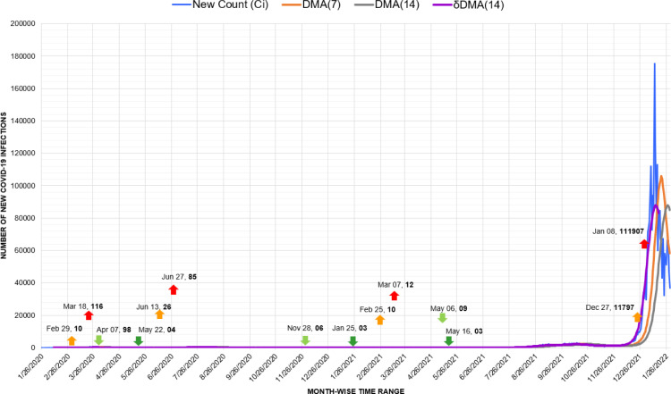
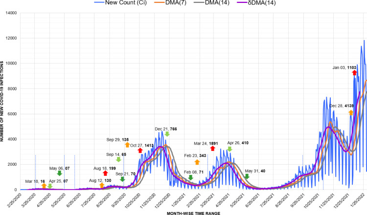
Australia exemplifies one of the stark instances of the suppression of previous waves due to the rise in counts caused by the Omicron variant. As visible in Fig. 14, the peaks of the first and second waves observed in March and June of 2020 had merely 18 and 27 new counts, respectively. Similarly, the peak in March 2021 witnessed the highest count of 12 cases. Synonymous with New Zealand, in Australia also, geographic isolation, relatively higher testing rates, and early implementation of social distancing measures were among the potential factors of successful response [49]. Yet, later these figures transmuted to a flat line against the trigger of 11,797 infections recorded for the fourth wave in December 2021.
Fig. 14.
Timeline graph of new Covid-19 infection cases in Australia.
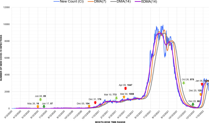
In Cuba, Covid-19 infection arrived with 3 Italian tourists in March 2020. With prompt sealing of borders, mandating face masks, and isolation of the infected population, Cuba responded to the pandemic successfully till November [50]. But, later, a nominal up-trigger of 104 cases observed on December 05, 2020, erupted into a devastating wave from June to December 2021 (Fig. 15). Here, the shift of decimal base was recorded as an up-trigger of 1008 cases on March 30 and a spike of 1047 cases on April 09, 2021.
Fig. 15.
Timeline graph of new Covid-19 infection cases in Cuba.
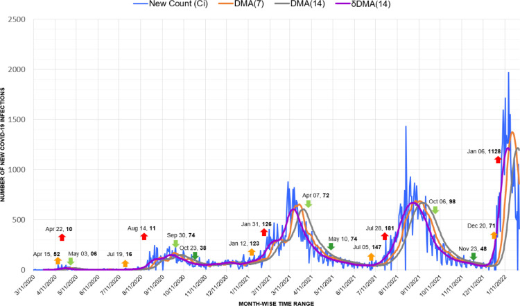
Before the first minor spike of 10 cases on 22 April, Jamaican authorities advised wearing masks only for persons over 65 years and individuals with symptoms or respiratory vulnerabilities [51]. Due to such misjudged policies, similar to Colombia, Jamaica also observed clear phases of Covid-19 waves, with each wave surpassing the records of the previous ones. The markers of our approach effectively depicted the triggers, spikes, and drops of each wave. Here also, the Omicron variant caused an unprecedented spike of 1128 infections in January 2022 (Fig. 16).
Fig. 16.
Timeline graph of new Covid-19 infection cases in Jamaica.
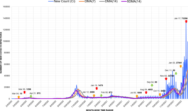
In Belgium, after responding successfully to the first peak, the start of educational year in academic institutions and the return of summer tourists from across the borders initiated the peak of October 2020 [52]. However, alike Australia, Belgium presents another case of suppressed previous waves by the latest wave in January 2021 (Fig. 17). Against a trivial spike of 1298 infections in March 2020, the trigger of 27,941 cases recorded in January 2021 resulted in an unprecedented Covid infection wave.
Fig. 17.
Timeline graph of new Covid-19 infection cases in Belgium.
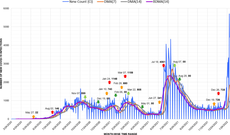
One of the most evident utilization of the trend generated by the DMA(14) model can be seen in the time-series graph of Croatia. Similar to New Zealand, the Croatian administration also employed a crisis management system for assessment and decision-making during the pandemic [53]. Here, extreme fluctuations are visible throughout each Covid-19 wave. These fluctuations indicate the rise of counts on one day and a sudden drastic drop within the next few days (Fig. 18.). The trends generated from these fluctuations have been analyzed appropriately by the DMA(14) model. The last and the highest wave in Croatia was recorded with an up-trigger of 4139 cases on December 28, 2021.
Fig. 18.
Timeline graph of new Covid-19 infection cases in Croatia.
Due to increased transmission vulnerability, political instability, and an inferior infrastructure for food and medical facilities, Libya has been placed among high-risk zones of the Covid pandemic [54]. Consequently, a significant observation in Libya was multiple drops to zero infection cases in many waves. A plausible reason for this absence of numbers may be the lack of information or the deficiency of medical testing facilities in the region. However, our DMA(14) model could still map a well-matched trend against these fluctuating counts. Until the writing of this manuscript, the latest and highest wave of infections was in its initial rising phase in Libya (Fig. 19).
Fig. 19.
Timeline graph of new Covid-19 infection cases in Libya.
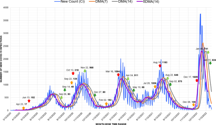
Kenya can be viewed as a case with the most evidently visible Covid-19 infection waves. Similar to Jamaica, every wave in Kenya shows a clear rise and fall of counts to visible limits in time series. Each wave has been marked with triggers, spikes, and drops by our approach (Fig. 20). Here, the third and fourth waves recorded a similar extent of damage, while the fourth wave depicted the highest count of 741 new infections on January 09, 2022. However, in addition to the nationwide educational media campaigns for promoting the usage of masks and handwashing, the Kenyan government also provided financial support to the local informal business sector for establishing sanitization mechanisms and handwashing stations through recycled and raw materials [55].
Fig. 20.
Timeline graph of new Covid-19 infection cases in Kenya.
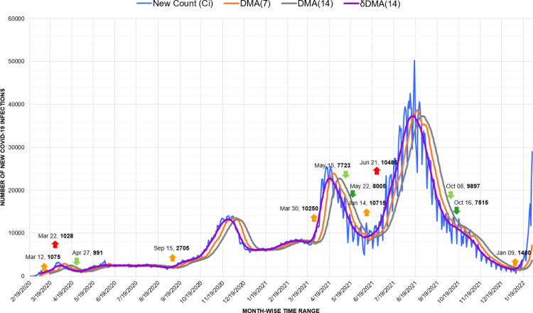
In terms of Asian countries, the Covid timeline of Iran displays a sharp rise of the first wave with an up-trigger of 1075 cases on March 12, 2020. A spike of 1028 infections confirmed the forecast for this wave on March 22 (Fig. 21). If this spike could have been handled, the first wave might have been averted. A steady drop in this wave was also recorded in April 2020. However, if this level of counts could have been maintained or lowered by precautionary measures, then the next up-trigger of 2705 cases on September 15, 2020, possibly could not have resulted in the next wave of infections. Here, despite early reports of the outbreak, the government’s sluggish response due to ideology and cynicism was a major factor behind this state of the pandemic. However, make-shift treatment centers and field hospitals in stadiums, wedding halls, and parking lots across the country have been established now to respond to the rapid spread of infection [56].
Fig. 21.
Timeline graph of new Covid-19 infection cases in Iran.
A lockdown during the traditional new year holidays in April helped Myanmar suppress the infection rate despite an inferior infrastructure [57]. Still, due to poor cooperation of the local population, Myanmar saw an up-trigger of 18 cases on August 19, 2020, which, with a spike of 148 infections on September 05, resulted in the first wave. The spike on May 24, 2021, evolved into another sharp wave (Fig. 22). However, this wave later exhibited a steady decline to the drop marker of 799 cases on October 28, 2021. Our proposed approach effectively logged the behavior of each wave with trends and markers in the time series of Myanmar.
Fig. 22.
Timeline graph of new Covid-19 infection cases in Myanmar.
6.3. Observation window
As discussed in Section 5.2, the length of an observation window (w) plays a significant role in the smoothing of values by a moving average model. It can be stated as the exact gap by which the projected values lead or lag the actual counts. Here, a larger value of w depicts a broader range of data points available for the distribution of data fluctuations by averaging. However, this large value will also increase the gap between the actual and forecasted values. Contrarily, a window (w) of a shorter gap will result in more fragmented trends and skipping of markers.
Thus, due to this reason, our proposed approach required a value of w that could project the smoothed changes in infection counts without any critical lag of time. Therefore, we selected a range of 7 to 14 days of the Covid-19 incubation period as an observation window. For forecasting the upcoming counts, the SMA(7) model sums up the average of the previous 7 errors and adds it to the corresponding result of classical SMA(7). This addition of errors covers the gap between projected and actual values to a much better extent compared to other baseline techniques. Elongation of w into a SMA(14) model will generate a forecast 7 days later compared to SMA(7), which may lead to missing critical changes in a wave.
Similarly, a backward displacement of DMA values by 14 units matches the trend projected by DMA(14) perfectly with the actual wave of infection counts. This length of displacement also makes the analysis of current trend more reliable despite short-timed spikes and drops in counts. A forecast model like DMA(7) with w reduced by 7 days will generate more fluctuating trends compared to DMA(14), leading to the skipping of critical markers in a wave. Equally, any further forward displacement higher than 14 days will place the trend far ahead in the timeline, thus impacting its credibility. Also, a longer recessive displacement will position the trend much backward compared to the actual counts rendering it useless for a forecast.
Therefore, we can deduce that the average of errors plays the same role in SMA(7) that the backward displacement of 14 days plays for DMA(14). We can also infer that any further extension of w will impact the forecast performance of models.
6.4. Implication of markers
This paper proposes 4 types of markers, namely spikes (s), drops (d), up-triggers (), and down-triggers (), for determining any significant change in the state of a Covid infection wave. As elaborated in Sections 3, 4, these markers work on shifting the decimal base of infection counts. Here, a few points about these markers need to be elucidated.
The first question arises about the length of the observation window (w) for detecting a marker. The purpose of setting it to 7 days has been stated earlier that it is the lower limit of the incubation period advised by the WHO [42]. Within this time, the first change in infection counts can be visible at the earliest, which can help societies, governments, and medical professionals to efficiently manage and re-allocate facilities for a possible change in numbers.
The second concern arises about the placement of spikes after up-triggers and drops after down-triggers. Here, it can be observed in the timeline charts of countries that after a trigger, there may be multiple increments and decrements in the infection count. Practically, these spikes and drops are responsible for the changing behavior of a Covid-19 infection wave. However, as visible from the timelines of New Zealand and Myanmar, if the first up-trigger is properly dealt with, further spikes can be suppressed effectively for a long time.
Another question that needs attention is the logic of generating markers. As we have explained earlier, a marker is generated at the rise or fall of the decimal base of infection counts. This implies that an up-trigger of 11,449 infections was generated on April 01, 2021, in the timeline of Colombia when the numbers crossed the 10,000 mark. However, no further spikes were registered as the decimal base did not change further up to 100,000 or higher numbers. In practical terms, the wave actually continued with multiple local rises and falls until the first down-trigger of 8503 cases was visible on July 26. Generation of any marker prior to this point might have resulted in further elongation of the wave. Hence, we can conclude that the logic of decimal base shift for generating markers confirms to the nature and lethality of the pandemic. However, to further ensure the behavior of a pandemic wave, the trend values (T[D]) generated by the DMA(14) function must also be considered. A sustained positive or negative change in these trend values is a strong indicator of wave behavior.
In Table 6, we have presented the forecast performance of our approach. It depicts the precision of the markers generated by the DMA(14)-base shift model. With the highest precision of 97.43% recorded for Jamaica and the lowest of 84.37% for Australia, our approach exhibited a fairly high average forecast performance of 94.08% for time series data of 12 countries.
Table 6.
Forecast precision performance of markers.
| Continent | Country | Forecast precision (%) |
|---|---|---|
| North America | Argentina | 94.594 |
| Colombia | 93.75 | |
| Oceana | New Zealand | 95.83 |
| Australia | 84.375 | |
| South America | Cuba | 90 |
| Jamaica | 97.435 | |
| Europe | Belgium | 94.594 |
| Croatia | 98 | |
| Africa | Libya | 96.428 |
| Kenya | 95.454 | |
| Asia | Iran | 94.44 |
| Myanmar | 94.117 | |
| 94.08475 | ||
6.5. Selection of MA models
We have already conferred over the forecasting limits of dedicated computational models [13], [14], [15] and ARIMA models [16], [17]. Here, the attempts to forecast Covid-19 infections by making use of advanced paradigms like machine learning methods also lead to similar outcomes. This implies that, similar to previous approaches, techniques such as deep learning [58], XGboost [59], support vector machines, and regression [60] are also dependent on the generation of pre-computed forecast models. These models require massive volumes of data for computations leading to hardware restrictions, timeline concerns, and scalability issues. Moreover, life-critical data with abrupt surges in numbers like Covid-19 infection counts require a flexible and speedy computational technique that can perform swiftly over any data size. Hence, we have proposed a method capable of executing over the time series data of Covid-19 infections in a walk-forward approach. This implies that our proposed models constantly upgrade with the changes in the infection counts, leading to more sensitive and accurate forecasts about upcoming and ongoing infection waves. We dedicate this section to justify the selection of moving average models employed for specific forecasting tasks.
Earlier in Section 2.2, we elaborated that a moving average is a weighted or unweighted mean of a set of data points. We also know that several application-specific variants of moving averages are available. However, the Covid-19 data is undeniably one of the most random-natured non-stationary time series available today. The absence of any trend or seasonality in this data makes the implementation of an exponential [32], [33] or weighted moving average [31], [34] model enormously challenging. Hence, we are left with the option of simple unweighted moving averages.
An unweighted moving average is an estimate of the expected values of the upcoming data points in the series. It works on the property that this estimation must be approximately similar to the values falling in the range of data points consumed for generating the mean. This property enables the forecast of upcoming values in a time series according to the constantly changing numbers. SMA(7) employs this property to forecast the next-day count of new Covid-19 infections.
The moving average of data points also generates a ‘smoothed’ version of the original values. Here, smoothing implies an even distribution of any temporal fluctuation in values among the component data points during the average calculation. This ‘smoothing’ property of moving averages is useful for DMA models in overcoming the spikes and drops of the Covid time series data. As depicted in Fig. 8., the DMA(14) models level off all fluctuations in the time series data in a manner much better than DMA(7) models. The DMA(14) model further improves this smoothing by dragging it backward to match the ongoing real-time trend of infection counts.
6.6. Deployment and utilization
The framework proposed in this paper can be implemented as an independent application or a micro add-on to an existing one. The emphasis of this framework is on the nearest forecast timeline of Covid impact in a region. Hence, it can be utilized by analysts, medical authorities, and administrative bodies for estimation of the upcoming state of the Covid-19 pandemic in their region. This estimation will be vital in the timely procurement, management, and allocation of medical infrastructure and healthcare resources like medical oxygen, hospital beds, and medicines. It will also assist governing bodies in designing and implementing time-bound precautionary measures and guidelines such as sealing of borders, social distancing, and wearing masks for the population under threat.
7. Conclusion & future work
In this paper, we proposed a novel algorithmic framework to forecast the wave behavior and upcoming counts of new Covid-19 infections in a region under a minimum observation window of 7 days. We have implemented this framework on a time series database of Covid-19 infections derived from 12 countries. The framework primarily comprises a displaced double moving average (DMA) algorithm and a novel ’corrected moving average’ ( SMA) technique.
The framework projects the rise and fall in Covid-19 waves by detecting potential dates with specific counts called ‘markers’ guided by decision rules mapped through rough set theory. In combination with the positive or negative trend computed by the DMA(14) algorithm, these counts can be classified into triggers, spikes, and drops of an infection wave with high accuracy.
Likewise, the corrected moving average ( SMA) algorithm computes the upcoming counts of new infections for the next day by adding the average error among the forecasted and actual counts to the upcoming forecasts. This addition of errors further corrects the forecasts, thus improving their next-day forecast precision up to 94.08%.
However, the proposed methods currently utilize predefined and constant window periods. We anticipate to improve the forecasting abilities of our framework with dynamically refreshable displacement and window periods of the component algorithms. We also intend to expand its coverage by implementing it over Covid-19 data of more countries in the future. We hope that the framework proposed in this manuscript proves itself supportive to the medical organizations and administrative authorities in allocating and managing healthcare infrastructure and medical facilities.
CRediT authorship contribution statement
Saurabh Ranjan Srivastava: Conceptualization, Data curation, Formal analysis, Investigation, Writing – original draft. Yogesh Kumar Meena: Conceptualization, Formal analysis, Project administration, Resources, Supervision, Validation, Review & editing. Girdhari Singh: Formal analysis, Resources, Supervision, Validation, Review & editing.
Declaration of Competing Interest
The authors declare that they have no known competing financial interests or personal relationships that could have appeared to influence the work reported in this paper.
Acknowledgments
The authors thank the editors and the anonymous reviewers for their helpful comments and suggestions. This work has been supported by the Science and Engineering Research Board (SERB) under the Department of Science & Technology, Government of India, for the project ’Forecasting Significant Social Events by Predictive Analytics Over Streaming Open Source Data’ (Project File Number: EEQ/2019/000697).
Biographies

Saurabh Ranjan Srivastava is a doctoral research scholar in the Department of Computer Science & Engineering at Malaviya National Institute of Technology Jaipur, India.
His areas of research are Data Mining & Spatiotemporal Forecasting.

Dr. Yogesh Kumar Meena is currently working as Associate Professor in the Department of Computer Science & Engineering at Malaviya National Institute of Technology Jaipur, India.
He received his Ph.D. in Computer Engineering from Malaviya National Institute of Technology Jaipur, India.
His research interests are Natural Language Processing, Information Retrieval, Data Mining and Neural Networks.

Dr. Girdhari Singh is currently working as Professor in the Department of Computer Science & Engineering at Malaviya National Institute of Technology Jaipur, India.
He received his Ph.D. in Computer Engineering from Malaviya National Institute of Technology Jaipur, India.
He is the author of textbooks on Software Engineering. His research interests are Software Engineering and Intelligent Systems.
Data availability
Data will be made available on request.
References
- 1.Hu B., Guo H., Zhou P., Shi Z.L. Characteristics of SARS-CoV-2 and COVID-19. Nat. Rev. Microbiol. 2021;19(3):141–154. doi: 10.1038/s41579-020-00459-7. [DOI] [PMC free article] [PubMed] [Google Scholar]
- 2.Maital S., Barzani E. The global economic impact of Covid-19: A summary of research. Samuel Neaman Inst. Natl. Policy Res. 2020;2020:1–12. [Google Scholar]
- 3.de Villiers C.B., Blackburn L., Cook S., Janus J. 2021. Sars-cov-2 variants. https://www.finddx.org/wp-content/uploads/2021/03/COVID-variants-report-FINAL-12MAR2021.pdf. [Google Scholar]
- 4.Zhang S.X., Marioli F.A., Gao R., Wang S. A second wave? what do people mean by covid waves? – a working definition of epidemic waves. Risk Manag. Healthcare Policy. 2021;14:3775. doi: 10.2147/RMHP.S326051. [DOI] [PMC free article] [PubMed] [Google Scholar]
- 5.Karim S.S.A., Karim Q.A. Omicron sars-cov-2 variant: a new chapter in the Covid-19 pandemic. Lancet. 2021;398(10317):2126–2128. doi: 10.1016/S0140-6736(21)02758-6. [DOI] [PMC free article] [PubMed] [Google Scholar]
- 6.Joshi S., Parkar J., Ansari A., Vora A., Talwar D., Tiwaskar M., Patil S., Barkate H. Role of favipiravir in the treatment of Covid-19. Int. J. Infect. Dis. 2021;102:501–508. doi: 10.1016/j.ijid.2020.10.069. [DOI] [PMC free article] [PubMed] [Google Scholar]
- 7.Felsenstein S., Herbert J.A., McNamara P.S., Hedrich C.M. Covid-19: Immunology and treatment options. Clin. Immun. 2020;215 doi: 10.1016/j.clim.2020.108448. [DOI] [PMC free article] [PubMed] [Google Scholar]
- 8.Narin A., Kaya C., Pamuk Z. Automatic detection of coronavirus disease (Covid-19) using x-ray images and deep convolutional neural net-works. Pattern Anal. Appl. 2021;24(3):1207–1220. doi: 10.1007/s10044-021-00984-y. [DOI] [PMC free article] [PubMed] [Google Scholar]
- 9.Pradhan D., Biswasroy P., Naik P.K., Ghosh G., Rath G. A review of current interventions for Covid-19 prevention. Arch. Med. Res. 2020;51(5):363–374. doi: 10.1016/j.arcmed.2020.04.020. [DOI] [PMC free article] [PubMed] [Google Scholar]
- 10.Bayyurt L., Bayyurt B. 2020. Forecasting of covid-19 cases and deaths using arima models. medrxiv. [Google Scholar]
- 11.Sahai A.K., Rath N., Sood V., Singh M.P. ARIMA modelling & forecasting of Covid-19 in top five affected countries. Diabetes Metabol. Syndrome Clin. Res. Rev. 2020;14(5):1419–1427. doi: 10.1016/j.dsx.2020.07.042. [DOI] [PMC free article] [PubMed] [Google Scholar]
- 12.Perc M., Gorisek Miksic N., Slavinec M., Stozer A., Covid Forecasting. 19. Front. Phys. 2020;8:127. [Google Scholar]
- 13.Fanelli D., Piazza F. Analysis and forecast of COVID-19 spreading in China Italy and France. Chaos Solitons Fractals. 2020;134 doi: 10.1016/j.chaos.2020.109761. [DOI] [PMC free article] [PubMed] [Google Scholar]
- 14.Anastassopoulou C., Russo L., Tsakris A., Siettos C. Data-based analysis, modelling and forecasting of the Covid-19 outbreak. PLoS One. 2020;15(3) doi: 10.1371/journal.pone.0230405. [DOI] [PMC free article] [PubMed] [Google Scholar]
- 15.Sarkar K., Khajanchi S., Nieto J.J. Modeling and forecasting the Covid-19 pandemic in India. Chaos Solitons Fractals. 2020;139 doi: 10.1016/j.chaos.2020.110049. [DOI] [PMC free article] [PubMed] [Google Scholar]
- 16.Hernandez-Matamoros A., Fujita H., Hayashi T., Perez-Meana H. Forecasting of Covid-19 per regions using ARIMA models and polynomial functions. Appl. Soft Comput. 2020;96 doi: 10.1016/j.asoc.2020.106610. [DOI] [PMC free article] [PubMed] [Google Scholar]
- 17.Petrica A.C., Stancu S., Tindeche A. Limitation of ARIMA models in financial and monetary economics. Theor. Appl. Econ. 2016;23(4) [Google Scholar]
- 18.Stein R.M. Moody’s KMV; New York: 2002. Benchmarking Default Prediction Models: Pitfalls and Remedies in Model Validation; p. 20305. [Google Scholar]
- 19.Pawlak Z. Springer Science & Business Media; 1991. Rough Sets: Theoretical Aspects of Reasoning About Data, 9. [Google Scholar]
- 20.Pawlak Z., Grzymala-Busse J., Slowinski R., Ziarko W. Rough sets. Commun. ACM. 1995;38(11):88–95. [Google Scholar]
- 21.Pawlak Z. Rough sets. Int. J. Comput. Inf. Sci. 1982;11(5):341–356. [Google Scholar]
- 22.Hill T., Marquez L., O’Connor M., Remus W. Artificial neural network models for forecasting and decision making. Int. J. Forecast. 1994;10(1):5–15. [Google Scholar]
- 23.Pawlak Z. Rough sets and decision analysis. INFOR: Inf. Syst. Oper. Res. 2000;38(3):132–144. [Google Scholar]
- 24.Lu Y., Xu Y., Huang J., Wei J., Herrera-Viedma E. Social network clustering and consensus-based distrust behaviors management for large-scale group decision-making with incomplete hesitant fuzzy preference relations. Appl. Soft Comput. 2022;117 [Google Scholar]
- 25.Kaliszewski I. Springer Science & Business Media; 2006. Soft Computing for Complex Multiple Criteria Decision Making, vol. 85. [Google Scholar]
- 26.Xu Y., Li M., Chiclana F., Herrera-Viedma E. Multiplicative consistency ascertaining, inconsistency repairing, and weights derivation of hesitant multiplicative preference relations. IEEE Trans. Syst. Man Cybern. Syst. 2021 [Google Scholar]
- 27.Ihaka R. 2005. Time series analysis. [Google Scholar]
- 28.Lim B., Zohren S. Time-series forecasting with deep learning: a survey. Phil. Trans. R. Soc. A. 2021;379(2194) doi: 10.1098/rsta.2020.0209. [DOI] [PubMed] [Google Scholar]
- 29.Jiang W. Applications of deep learning in stock market prediction: recent progress. Expert Syst. Appl. 2021;184 [Google Scholar]
- 30.Sahin U., Balli S., Chen Y. Forecasting seasonal electricity generation in European countries under Covid-19-induced lockdown using fractional grey prediction models and machine learning methods. Appl. Energy. 2021;302 doi: 10.1016/j.apenergy.2021.117540. [DOI] [PMC free article] [PubMed] [Google Scholar]
- 31.Box G.E., Jenkins G.M. Time Series Analysis: Forecasting and Control. Holden-Day; 1976. [Google Scholar]
- 32.Gardner Jr. E.S. Exponential smoothing: The state of the art. J. Forecast. 1985;4(1):1–28. [Google Scholar]
- 33.Winters P.R. Forecasting sales by exponentially weighted moving aver-ages. Manage. Sci. 1960;6(3):324–342. [Google Scholar]
- 34.Harvey A.C. Cambridge University Press; 1990. Forecasting, Structural Time Series Models and the Kalman Filter. [Google Scholar]
- 35.Hyndman R.J. Citeseer; 2011. Moving Averages. [Google Scholar]
- 36.Vandewalle N., Ausloos M., Boveroux P. The moving averages demystified. Physica A. 1999;269(1):170–176. [Google Scholar]
- 37.Alevizakos V., Chatterjee K., Koukouvinos C., Lappa A. A double moving average control chart: discussion. Comm. Statist. Simulation Comput. 2020:1–15. [Google Scholar]
- 38.Mustapa R., Latief M., Rohandi M. International Conference on Education, Science and Technology. Redwhite Press; 2019. Double moving average method for predicting the number of patients with dengue fever in gorontalo city; pp. 332–337. [Google Scholar]
- 39.2022. Displaced moving average. https://www.incrediblecharts.com/indicators/displacedmovingaverage.php (Accessed 06 February 2022) [Google Scholar]
- 40.2022. Our world in data. https://ourworldindata.org (Accessed 02 February 2022) [Google Scholar]
- 41.Khoo M.B., Wong V. A double moving average control chart. Commun. Stat. Simul. Comput. 2008;37(8):1696–1708. [Google Scholar]
- 42.2022. The 14-day quarantine: Understanding the coronavirus incubation period. https://www.pfizer.com/foundations-science/14-Day-Quarantine-Incubation-Period. (Accessed 06 February 2022) [Google Scholar]
- 43.Zaki N., Mohamed E.A. The estimations of the covid-19 incubation period: A scoping reviews of the literature. J. Infect. Publ. Health. 2021;14(5):638–646. doi: 10.1016/j.jiph.2021.01.019. [DOI] [PMC free article] [PubMed] [Google Scholar]
- 44.Stobart A., Duckett S. Australia’s response to Covid-19. Health Econ. Policy Law. 2022;17(1):95–106. doi: 10.1017/S1744133121000244. [DOI] [PMC free article] [PubMed] [Google Scholar]
- 45.Khair U., Fahmi H., Al Hakim S., Rahim R. Forecasting error calculation with mean absolute deviation and mean absolute percentage error. J. Phys. Conf. Ser. 2017;930 [Google Scholar]
- 46.Gemelli N.A. Management of COVID-19 outbreak in Argentina: the beginning. Disaster Med. Publ. Health Preparedness. 2020;14(6):815–817. doi: 10.1017/dmp.2020.116. [DOI] [PMC free article] [PubMed] [Google Scholar]
- 47.Prada S.I., Garcia-Garcia M.P., Guzman J. COVID-19 response in Colombia: Hits and misses. Health Policy Technol. 2022 doi: 10.1016/j.hlpt.2022.100621. [DOI] [PMC free article] [PubMed] [Google Scholar]
- 48.Dyer P. Brookings Doha Centre; 2021. Policy and Institutional Responses to COVID-19: New Zealand; pp. 1–25. [Google Scholar]
- 49.O’Sullivan D., Rahamathulla M., Pawar M. The impact and implications of COVID-19: An Australian perspective. Int. J. Commun. Soc. Dev. 2020;2(2):134–151. [Google Scholar]
- 50.Wylie L.L. Cuba’s response to COVID-19: lessons for the future. J. Tourism Futures. 2021 [Google Scholar]
- 51.Amour R., Robinson J., Govia I. The COVID-19 long-term care situation in jamaica, ltccovid. Int. Long-Term Care Policy Netw. 2020 [Google Scholar]
- 52.Natalia Y.A., Faes C., Neyens T., Molenberghs G. The COVID -19 wave in Belgium during the fall of 2020 and its association with higher education. PLoS One. 2022;17(2) doi: 10.1371/journal.pone.0264516. [DOI] [PMC free article] [PubMed] [Google Scholar]
- 53.Srbljinovic A., Bozic J., Fath B.D. Croatian crisis management system’s response to COVID -19 pandemic through the lens of a systemic resilience model. Interdiscip. Descript. Complex Syst. INDECS. 2020;18(4):408–424. [Google Scholar]
- 54.Iwendi G.C., Alsadig A.M., Isa M.A., Oladunni A.A., Musa M.B., Ahmadi A., Adebisi Y.A., D. E. Lucero-Prisno III. COVID -19 in a shattered health system: Case of Libya. J. Global Health. 2021;11 doi: 10.7189/jogh.11.03058. [DOI] [PMC free article] [PubMed] [Google Scholar]
- 55.Wangari E.N., Gichuki P., Abuor A.A., Wambui J., Okeyo S.O., Oyatsi H.T., Odikara S., Kulohoma B.W. Kenya’s response to the COVID -19 pandemic: a balance between minimizing morbidity and adverse economic impact. AAS Open Res. 2021;4 doi: 10.12688/aasopenres.13156.1. [DOI] [PMC free article] [PubMed] [Google Scholar]
- 56.Ebrahimi M., Gassama S.K., bin Yusoff K. COVID -19: Threat and response in Iran. Iran Caucasus. 2020;24(4):423–443. [Google Scholar]
- 57.Oo M.M., Tun N.A., Lin X., D. E. Lucero-Prisno III. COVID -19 in myanmar: Spread actions and opportunities for peace and stability. J. Glob. Health. 2020;10(2) doi: 10.7189/jogh.10.020374. [DOI] [PMC free article] [PubMed] [Google Scholar]
- 58.Suganya R., Kanmani R., Joyal S.G., G S. Advanced deep learning model for future forecasting of covid-19. J. Phys. Conf. Ser. 2021;1916(1):012147. [Google Scholar]
- 59.Tahsin L., Roy S. Prediction of Covid-19 severity level using xgboost algorithm: a machine learning approach based on SIR epidemical model. EasyChair. 2021 [Google Scholar]
- 60.Parhusip H.A. Study on COVID-19 in the world and Indonesia using regression model of SVM bayesian ridge and gaussian. J. Ilmiah Sains. 2020;20(2):49–57. [Google Scholar]
Associated Data
This section collects any data citations, data availability statements, or supplementary materials included in this article.
Data Availability Statement
Data will be made available on request.


