

Abstract

The hydrophobicity of oils is a key parameter to design surfactant/oil/water (SOW) macro-, micro-, or nano-dispersed systems with the desired features. This essential physicochemical characteristic is quantitatively expressed by the equivalent alkane carbon number (EACN) whose experimental determination is tedious since it requires knowledge of the phase behavior of the SOW systems at different temperatures and for different surfactant concentrations. In this work, two mathematical models are proposed for the rapid prediction of the EACN of oils. They have been designed using artificial intelligence (machine-learning) methods, namely, neural networks (NN) and graph machines (GM). While the GM model is implemented from the SMILES codes of a 111-molecule training set of known EACN values, the NN model is fed with some σ-moment descriptors computed with the COSMOtherm software for the 111-molecule set. In a preliminary step, the leave-one-out algorithm is used to select, given the available data, the appropriate complexity of the two models. A comparison of the EACNs of liquids of a fresh set of 10 complex cosmetic and perfumery molecules shows that the two approaches provide comparable results in terms of accuracy and reliability. Finally, the NN and GM models are applied to nine series of homologous compounds, for which the GM model results are in better agreement with the experimental EACN trends than the NN model predictions. The results obtained by the GMs and by the NN based on σ-moments can be duplicated with the demonstration tool available for download as detailed in the Supporting Information.
1. Introduction
A large diversity of natural and synthetic liquid compounds are grouped under the generic term “oils” due to their non-miscibility with water. They are key components of surfactant/oil/water (SOW) systems such as swollen micelles, microemulsions, or emulsions which are found in numerous end-use products and various fields such as cosmetics, pharmaceutics, food, crude oil, and so forth. The quantitative evaluation of the hydrophobicity of the oil is extremely important because it allows for choosing the most effective SOW system composition and, in fine, optimizing its performances in applications.
Several concepts have thus been developed to characterize the hydrophobicity/polarity of oils. The best known are log P, that is, the logarithm of the n-octanol–water partition coefficient1 and the “required HLB” (hydrophilic–lipophilic-balance).2,3 Log P is widely used in environmental and medical sciences since it expresses the ability of a non-ionizable substance to partition between aqueous and lipophilic compartments of organisms, but it gives no indication regarding its behavior at the O/W interfaces in SOW systems.1 The required HLB value of an oil, introduced by Griffin,2,3 was designed to that aim. It corresponds to the HLB value of the mixture of surfactants providing the most stable emulsion with the oil under study.2,4 This method is sometimes used to classify complex mixtures such as essential, vegetable, or animal oils.5−9 However, the required HLBs thus obtained are imprecise and poorly reproducible because they depend on the mixture of surfactants and on the emulsification process. Furthermore, the required HLB concept is based on the HLB of surfactants which is itself an approximate empirical parameter only reliable for polyethoxylated nonionic surfactants.
A more relevant concept to quantify the hydrophobicity of an oil in SOW systems was introduced in 1977 by Wade et al. as a dimensionless number: the so-called equivalent alkane carbon number (EACN).10 It corresponds to the number of carbon atoms of the n-alkane that exhibits a phase behavior similar to that of the oil under consideration.11 In practice, measuring accurately the EACN value of an oil is tedious. The standard method is based on the elaboration of the so-called “fish diagrams,” which represent the phase behavior of equilibrated SOW systems where S is a well-defined polyethyleneglycol monoalkyl ether (CiEj for CH3(CH2)i−1O(CH2CH2O)jH) and the water-to-oil ratio (WOR) is equal to 1.12
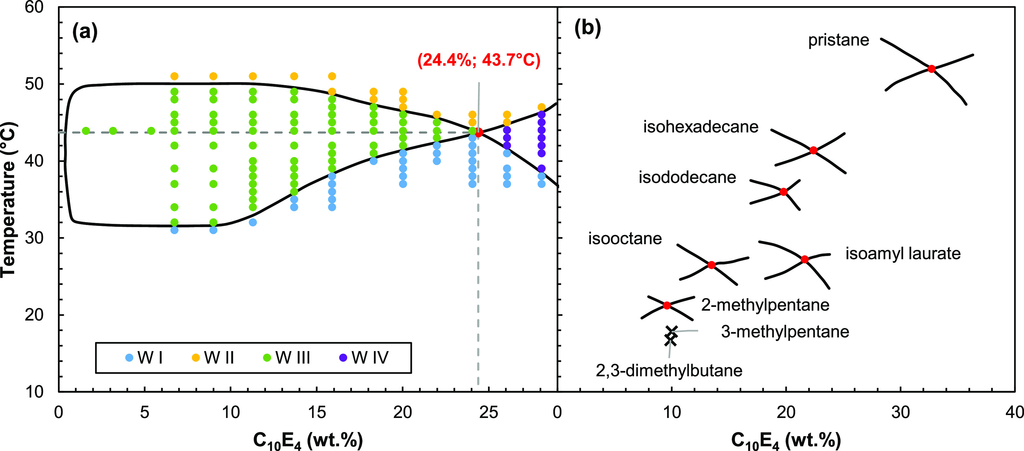
A typical fish diagram of a system C10E4/oil/water is given in Figure 1a as an example. When varying the temperature and the surfactant concentration, the CiEj/oil/water-T systems provide different types of microemulsion behaviors, called Winsor phases (Winsor I, II, III, and IV) depending on the affinity of the surfactant for water and oil. When it is balanced, a three-phase system (Winsor III) is formed, giving a diagram shaped like a fish. The characteristic temperature T* at the intersection of the Winsor I to IV (i.e., one single phase microemulsion) regions is then compared to the T* values of a series of n-alkanes (Figure 1b) to determine the EACN of the oil which expresses its hydrophobicity.11,13
Figure 1.

Determination of the EACN of an oil from the fish plot of the C10E4/oil/water-T system (a). The temperature of the fish-tail point indicated in red is reported to the calibration straight line obtained with C10E4/n-alkanes/water-T systems (b).
While reliable and accurate, the experimental determination of EACNs from fish tail diagrams is, however, a lengthy process which is limited by experimentally accessible conditions in terms of temperature (T ≈ 5–80 °C). Thus, in silico estimation of the EACN values of oils without any experiments would be considerably time-saving.
To date, a few predictive models of EACN values have been reported. The EACN value of complex oil mixtures, that is, crude oil, was predicted by Creton et al. using an evolutionary algorithm coupled to data mining.14 Bouton et al. built a QSPR model by applying genetic algorithms to structural molecular descriptors of polar hydrocarbon oils.15 A multilinear regression based on the σ-moments calculated by the conductor-like screening model for real solvents (COSMO-RS) approach16,17 was applied to polar hydrocarbons and aprotic polar oils by Lukowicz et al.18,19 These works showed that depending on the chemical functions of molecules, the relevant descriptors differ and EACN estimations were less satisfactory in the case of polar oils. Building a QSPR model relies on finding the best relation between a group of descriptors and a target property. Those models require the construction of a reliable database, consisting of entry/output pairs where entries are molecular descriptors and outputs are the target properties. Numerous predictive methods, based on linear and nonlinear approaches, have been applied to a diversity of physical and chemical properties.20 The linear methods, such as MLR, principal component regression, and partial least-squares regression, are often used. However, non-linear models can be adapted to translate more complex relations between descriptors and the predicted property, making them more efficient predictors in some cases.20−22 Rather than using methods that select descriptors from a large pull of automatically generated variables,21 we have chosen to start with descriptors that have a physical meaning, such as σ-moments (computed with COSMOtherm) and 2D structures of molecules used as descriptors for graph machines (GM).23 Already, a variety of chemical and physicochemical properties such as boiling point of halogenated hydrocarbons,24 surface tension,25 viscosity,26 flash point, cetane number of fuels,27 bioactivity of drugs,24,28 and other thermodynamic properties29−31 can be predicted accurately with GM and neural networks (NN) inputted with 2D-structures and σ-moments, respectively. Both these theoretical tools are non-linear models that learn a pathway from input values to a resulting output. For NNs, that are basically standard multi-layer perceptrons (MLPs), the inputs are either measured or computed from molecular simulations, while for GMs, the inputs are the 2D molecular structures entered as their SMILES (simplified molecular input line entry specification) codes.
In this work, we report on two approaches for predicting the EACN of functionalized oils using NN and GM. To that goal, a set of 111 molecules with a reliable experimental EACN was gathered either from literature or from our own database.11,15,18,19,32−34 A GM regression based solely on the readily accessible molecular SMILES codes and a NN regression using as inputs COSMO-RS-computed σ-moments are designed for the 111 molecules. After a selection step of the optimal model in each case, predictions are performed on a test set of 10 cosmetic or perfumery molecules for which experimental EACNs have been determined. The respective reliability of the two models is finally evaluated by predicting the EACN of compounds belonging to nine homologous series.
2. Materials and Methods
2.1. Database Construction
A set of 121 compounds with reliable EACN values either extracted from literature or determined experimentally in our laboratory was assembled. These averaged EACN values are reported in Table S1 of the Supporting Information. The whole set includes n-alkanes, esters, ethers, ketones, alkenes, alkynes, cyclic hydrocarbons, aromatics, branched hydrocarbons, nitriles, chloroalkanes, and consequently compounds containing carbon, hydrogen, oxygen, nitrogen, and chloride atoms. In addition to the commercially available series which are mainly linear compounds, the data set contains molecules of varying complexity, which are characterized by their structural features, that is, the presence of a double bond (alkene), ring, branching, and functional group. For training and testing purposes, this set was divided into a training set of 111 compounds and a test set of 10 compounds, including five cosmetic-type oils and five perfume-type oils. Among the five cosmetic oils, three compounds (hemisqualane, dioctylether, and isopropyl myristate) were already members of the test sets of our previous papers.25,26 Isododecane, a petroleum-based cosmetic, has recently been synthetized under environmentally friendly conditions, becoming thus an important molecule for cosmetic formulators and manufacturers. Finally, octyloctanoate was selected because it is the only ester with a functional group in the middle of its carbon skeleton. As for the five fragrance molecules, they were chosen because they have several structural characteristics: (i) one or two cycles, double bonds, and branching (limonene and caryophyllene), (ii) double bonds, branching, and an ester group (linalyl acetate), and (iii) a cycle, one or two double bonds, branching, and an ether or ketone function (rose oxide and β-ionone). In addition, the EACN values of these 10 compounds, which have been determined in our group to have consistent values, are fairly well distributed over the range of property values (−4 to 20). The distributions of the structural features present in both data sets are displayed in Figure 2, indicating clearly the challenging complexity of the test set molecules.
Figure 2.

Distribution of common structural features (in percent) of molecules in the training and test sets of the EACN database.
2.2. EACN Experimental Determination
2.2.1. Chemicals
Oils for which EACN values were measured in this work are presented in Table 1 and were used as such. Pure tetraethyleneglycol monodecyl ether (C10E4) was synthesized according to a method described elsewhere.35,36 Its purity was assessed by GC–MS analysis (>99%) and by comparing its cloud point temperature at 2.6 wt % (20.4 vs 20.6 °C) with the reference value.37 Tetraethyleneglycol monohexyl ether (C6E4) was synthetized using an analogous method to C10E4, and its cloud point temperature (66.2 °C at 16.4 wt %) was compared to the reference value (66.1 °C at 16.4 wt %).38
Table 1. Oils for Which EACN Values Were Measured in This Work, Commercial Name, Supplier, and Purity.
| compound | supplier | purity |
|---|---|---|
| isoamyl laurate, JOLEE 7750 | Oleon | 100% |
| hemisqualane, Neossance | Amyris | >95% |
| isohexadecane, 2,2,4,4,6,8-heptamethylnonane | Sigma-Aldrich | 98% |
| pristane, 2,6,10,14-tetramethylpentadecane | TCI | >95% |
| isododecane, 2,2,4,6,6-pentamethylheptane | TCI | >98% |
| 2-methylpentane | Sigma-Aldrich | >99% |
| 3-methylpentane | Sigma-Aldrich | >99% |
| 2,3-dimethylbutane | Sigma-Aldrich | 98% |
| isooctane, 2,2,4-trimethylpentane | Sigma-Aldrich | >99% |
| dipropyl ether | Sigma-Aldrich | >99% |
| diisopropyl ether | Sigma-Aldrich | >98.5% |
2.2.2. Phase Diagrams
In order to enrich the EACN values database, experimental phase diagrams were built, in particular in the case of branched alkanes that were under-represented in the literature data. The experimental EACN value was determined by establishing the phase behavior of 50 ± 0.2 wt % water/oil mixtures at different C10E4 or C6E4 concentrations as a function of temperature. The Winsor systems were determined by visual observation.39 The most volatile oil samples (2-methylpentane, 3-methylpentane, and 2,3-dimethylbutane) were weighed in glass tubes, placed in liquid nitrogen, and then sealed with a flame. Other samples were prepared in glass tubes closed by screw caps. Samples were first shaken gently several times and left in a thermoregulated bath at T ± 0.1 °C until equilibration. The point (C*; T*) corresponding to the intersection of the Winsor III and the Winsor IV phases was used to determine the oil’s EACN: its T* value was reported on the T* versus ACN reference straight line for linear alkanes using either C10E4 or C6E4 as the surfactant.11 The fish diagram of hemisqualane is given as an example in Figure 3a. The fish diagram lower concentration limit was determined by extrapolation of Winsor III phase relative volume as described by Burauer et al.40 Other experimentally determined (C*; T*) points using C10E4 are represented in Figure 3b. Fish diagrams of dipropylether and diisopropyl ether determined with C6E4 as a surfactant are available in Figures S1 and S2 of the Supporting Information.
Figure 3.
(a) Experimental fish plot of the C10E4/hemisqualane/water-T system at a water/oil ratio equal to 1 (w/w) and (b) partial fish plot and fish tail points (C*; T*) determined with C10E4 for pristane (2,6,10,14-tetramethylpentadecane), isohexadecane (2,2,4,4,6,6,8-heptamethylnonane), isododecane (2,2,4,6,6-pentamethylheptane), isooctane (2,2,4-trimethylpentane), isoamyl laurate (3-methylbutyl dodecanoate), and 2-methylpentane. Fish tail points (C*; T*) for 3-methylpentane and 2,3-dimethylbutane are represented by cross-marks for clarity.
2.3. COSMO-RS σ-Moment Calculation
COSMO-RS is a first-principles theoretical model based on a combination of quantum chemistry and statistical thermodynamics that serves to estimate, without any prior experience, a large number of chemical properties.17,41 Due to the presence of polar covalent bonds, molecules carry a surface charge density σ on its so-called “σ-surface”, which corresponds to the slightly inflated van der Waals surface. The “σ-profile” pX(σ) of a molecule X is the curve obtained by smoothing the histogram of surface portions grouped by charge density in the interval [σ – dσ/2, σ + dσ/2].16 Examples in the case of β-ionone and isopropyl myristate are represented in Figure 4. Using the COSMO-conf software (version 4.3), the lower energy conformations in the bulk liquid state are calculated for all molecules. These conformations are then used as inputs in the COSMOtherm software (version 19.0.4), allowing for the calculation of the σ-surface, σ-potential, and σ-moments. Klamt17 has shown that any partition coefficient K can be very well expressed as a Taylor-like development of σ-moments as defined by eq 1. It is estimated that a development up to m equal to six σ-moments is sufficient to satisfactorily express the partition coefficient K according to eq 1.
| 1 |
Figure 4.

σ-Profiles and σ-surfaces of β-ionone (in blue) and isopropyl myristate (in purple). The color gradient corresponds to the surface charge density σ.
The σ-moments MiX are calculated from the σ-profile pX(σ) of the studied compound X according to eqs 2–4.
| 2 |
| 3 |
| 4 |
The first σ-moments have a simple physical meaning: the zero-order σ-moment M0X is the surface area of the molecule, expressed in Å2. The first-order one M1 is the polarization charge of this surface, expressed in e. For uncharged molecules, this moment is equal to zero. The second-order σ-moment M2X, expressed in e2·Å–2, is the polarity of the molecule.42 The third-order M3 represents the asymmetry of the σ-profile pX(σ). The other σ-moments up to M6X have no particular physical meanings. Finally, Macc and MdonX, expressed in e (unit equal to the charge of one electron), are the “hydrogen-bonding” σ-moments representing the ability of the molecule to interact with hydrogen-bond acceptors and donors, respectively. Their value is non-zero when the σ-profile outranges the [−σHB, +σHB] interval, where σHB, the hydrogen-bond threshold, is equal to 0.01 e·Å–2, as shown in Figure 4.
Neither β-ionone nor isopropyl myristate exhibit Lewis acidity corresponding to the hydrogen-bond donor region. However, both of them have a Lewis basicity with non-zero-value σ-profile in the hydrogen-bond acceptor region. This is due to the presence of the ester and carbonyl functions inducing locally electron-rich surface areas (in red in both molecules according the color scale in Figure 4). Finally, the central part of the σ-profile shows higher hydrophobicity in the case of isopropyl myristate than for β-ionone, which is in accordance with its longer alkyl moiety.
2.4. GM and NN Model Selection
As briefly stated in the introduction, GM are regression or classification models that estimate a property directly from the topological information provided by their SMILES codes. In these models, molecules are described as directed acyclic graphs derived from their 2D structures and the parameterized functions that compute the estimate of the property of interest reflect the molecular structures of the compounds.28,43 As usual in regression or classification models, GM parameters are computed by learning from examples present in an experimental value database.28 Basically, NN models are multiple non-linear regressions that estimate an output value of a property of interest from some input descriptors values, hereafter three σ-moments selected from a pull of eight σ-moments, all computed with COSMO-RS according to a procedure described in Section 2.3. [A selection of the σ-moments was performed with Metagen, a homemade software package written in Python. Feature selection by the random probe method showed that for our data, M0X, M2, and M3X are most relevant for EACN estimation; n was also selected as relevant when added to the pull of σ-moment descriptors.]44 Both NN and GM models are built from MLPs that contain a single hidden layer of neurons. The complexity of the models is consequently dependent on the number of neurons of that layer, and along with this, on the number of parameters of the models. Since, for a given number of neurons in the MLPs, NN and GM models have a different number of parameters, the latter variable will be preferred as a complexity equivalent in the model complexity selection (Section 3.2).
The selection of a model is a key step in machine learning model design: it consists in finding the model complexity, given the available data for designing it, that will result in the best generalization. To that end, with the 111-molecule set available, trainings are carried out with an increasing number of MLP hidden neurons. The ability of both models to account for the training data is monitored with the root mean square training error (RMSTE) that is computed as follows
| 5 |
where EACNexp.i is the EACN value determined experimentally for molecule i, and EACNest. is the EACN value estimated by the model for molecule i at the end of the training.
The estimation of the generalization error for model selection is usually performed by two methods: the computation of the leave-one-out (LOO) score and the computation of the virtual LOO (VLOO) score. The computation of the LOO score was chosen for the determination of the optimal complexity, since the VLOO score, that is a first order approximation of the LOO score, is less accurate for small size data sets.26,45 At the end of the LOO process, the LOO score is computed as
| 6 |
where EACNexp.i is the EACN value determined experimentally for molecule i, and EACNpred. is the average EACN prediction value computed for the left out molecule i with 50 models having different initialization parameters. The abovementioned equation is the same as eq 5 defining the RMSTE, except that now a true prediction is performed for every molecule, since the molecule i does not belong to the training set. The LOO computation is repeated five times for each complexity of the NN and GM based models, so that the average results are presented.
A few difficulties have been met with the first modeling experiments that have been addressed as follows. With the σ-moment-based NN models, a large EACN deviation was observed specifically for the 15 molecules of the n-alkane family, regardless of the complexity of the MLPs used. We found that adding the number of carbon atoms (n) for every molecule as a fourth descriptor corrected this problem. Similarly, an important deviation from the experimental value was exclusively observed for the hexyl octanoate EACN estimation with the GM-based models. A thorough analysis of the GM construction for this molecule indicated that it was not consistent with the construction of the other linear ester GMs (e.g., the ethyl esters). The input code for ethyl hexanoate was particularized so that the constructions were uniform for all esters. This modification is explained in Figure 5 where the directed graphs for hexyl octanoate and ethyl dodecanoate are shown (a). These graphs, which are encoded from their SMILES codes (b), are isomorph to the 2D formula also represented (c). Without modification of the hexyl octanoate SMILES code, the central node of the resulting graph, also called root node, would have been located on the green node. Thanks to the special bracketed tag in the hexyl octanoate SMILES code, the graph red root nodes have now a consistent position in both graphs: the root nodes are equally connected to nodes with a carbon type label and are at the same distance of the functional node, which is the one connected to the nodes with an oxygen-type label. The position of the root node is important since it corresponds to the GM (not represented) output neuron that computes the estimated EACN value. As a result, the estimation of the EACN was much efficient for the hexyl octanoate compound.
Figure 5.

Encoding hexyl octanoate and ethyl dodecanoate into directed graphs: (a) directed graphs with root nodes in red; the root node position computed automatically for hexyl octanoate is colored in green and the path between the functional atom node and the root node in pink, (b) SMILES codes with the expected position of the root nodes indicated in red and (c) 2D formulas with expected positions for the root nodes (red arrows). The atom types C and O added on the directed graphs correspond to node labels that are inputs of the parameterized function implemented at each node of the graph to build the GM.
We did not meet such a particular case with our published models designed for surface tension and viscosity estimations.25,26 This is probably because we used a larger training set counting many esters of various sizes and positions for the functional group. For this work, we could only build a data set of moderate size, and among the dozen of linear esters that have an alkyl chain of 10 carbon atoms or more, hexyl octanoate is the unique compound of similar size in the training set to have a functional group in the middle of its carbon skeleton. To illustrate this exception, a representation of the GM can be computed with the demo software as detailed in the Supporting Information.
3. Results and Discussion
The EACN of an oil quantitatively expresses its hydrophobicity and corresponds to the related but obsolete concept of “required HLB” of oils introduced by Griffin in 1949.2,46 The more hydrophobic the oil, the higher its EACN. In particular, for the n-alkane series, the EACN is, by definition, equal to the carbon number of the alkane and is denoted ACN. Conversely, the more polar the oil, the lower its EACN and the EACN can even be negative for short oils bearing a polar function such as a ketone or a nitrile.
3.1. Theoretical Versus Experimental EACNs
In colloidal physical chemistry, the EACN value of an oil expresses its ability to penetrate the interfacial film of SOW systems and to modify its spontaneous curvature.47−49 In the case where the surfactant is a polyethoxylated fatty alcohol CiEj, some molecules of oil penetrate the interfacial film according to their affinity for CiEj molecules. In particular, when the oil has a polar function, its affinity for the film is stronger than apolar oils and its EACN is much lower than n, its number of carbon atoms. Indeed, Figure 6 illustrates the identical Winsor phase behavior of octyl octanoate (n = 16) and n-octane (n = 8), which is the linear alkane having an ACN equal to the EACN of the ester.
Figure 6.

Effect of oil penetration on the spontaneous curvature of the interfacial film (top) and C10E4/oil/water [WOR = 1 (v/v)] microemulsion systems equilibrated at 25.0 °C yielding Winsor II, Winsor III, and Winsor I microemulsions (bottom). Systems with n-alkanes contain 3% C10E4, and the one with octyl octanoate contains 7% C10E4.
The EACN concept is of interest only if the values assigned to oils do not depend on the nature of the CiEj surfactant used for its measurement. This key issue has been checked by Bouton et al. who showed that the EACN values of 26 terpenes and non-linear (branched, unsaturated, cyclic) hydrocarbons were identical within 0.3 unit regardless of the surfactant used, namely, C6E4, C8E4, or C10E4.15 However, for very polar oils, two major problems decrease the accuracy of EACN measurements. The first one stems from the fact that for oils having an EACN lower than 6, the calibration curve established with n-alkanes must be extrapolated to the dotted parts of the regression straight line (see Figure 1b). Accordingly, the lower the EACN, the greater the uncertainty over its estimated value. The second problem arises from the monomeric solubility of CiEj surfactants in the oil phase which increases the apparent polarity of the oil. As a result, the EACNs measured with short CiEj such as C6E4 tend to be lower than the EACNs measured with a long CiEj whose monomeric concentration in the oil phase is significantly lower. This issue is particularly acute when the oils are very polar and the CiEj is very short. We encountered this difficulty while seeking to model the EACN of diisopropyl ether, for which we had previously assigned an EACN equal to 2.212 on the basis of the fish diagram determined by Wormuth and Kaler with the C12E6/diisopropyl ether/water system.50 According to our very first models (GM and NN), the EACN of this oil appeared as an outlier. We therefore measured the EACN of this ether again using the same amphiphile (C6E4) that was used to measure the EACNs of most other highly polar oils.34 The new value of the EACN thus determined (0.6, see Supporting Information) is, as expected, significantly lower than the previous value and perfectly consistent with the EACNs of other very polar oils, as they were determined with the same surfactant (C6E4). This revised EACN value has therefore been used to fit our GM and NN models.
3.2. GM and NN Complexity Selection
Figure 7 which displays the LOO scores and RMSTE versus the number of parameters of the MLPs, that is the complexity, for the GM and NN models, indicates that in both cases (i) the data are correctly learned since the RMSTE are decreasing monotonously as the complexity increases and (ii) the LOO scores decrease, go through a minimum, and start increasing. The NN LOO score is clearly minimum (0.8 EACN unit) for a number of parameters equal to 37, that is, six hidden neurons. On the contrary, very close GM LOO score values equal to 0.8 and 0.9 EACN unit are computed for 45 (5N) and 58 (6N) parameters, respectively. In such a situation, the usual practice is to select the model with the lower complexity.30 Therefore, GMs with five hidden neurons (45 parameters) and NNs with six hidden neurons (37 parameters) were kept for later testing.
Figure 7.

RMSTE value of the model (out of 1000) having the smallest RMSTE for the GM-based model (orange empty diamonds) and NN-based model (blue circles) for the 111 molecules of the training set and means of the LOO score values (GM orange diamonds, NN blue-filled circles) computed for five different parameter initializations for the 111 molecules of the training set vs number of parameters. The error bars for the LOO scores are the standard deviations computed over the five LOO score values.
An alternative to the LOO score computation is the leave-many-out (LMO) score computation, for which several molecules (e.g., k) are removed from the training set instead of one. Since the data set is small, it is advisable to train as many examples as possible to avoid overfitting. Indeed, when the number of parameters of the trained model exceeds half the number of examples in the training set, overfitting occurs and prediction performance starts deteriorating (above 60 parameters in Figure 7). With LOO, more examples are trained than with LMO (110 rather than 111–k), which reduces the risk of overfitting for a given number of parameters. Furthermore, with LOO, the maximum amount of information is used for training in the case of each removed example, so that the highest possible accuracy for its predicted value can be expected. Therefore, LOO was preferred to LMO, even if it requires a little more computation time.
For comparison purposes, the results of the EACN LOO estimations, corresponding to the LOO computation (out of five) that gives the best LOO score (0.8 EACN unit for GM and NN) for the molecule training set versus experimental EACN, are displayed in Figure 8 for the two preferred models.
Figure 8.

Scatter plots of LOO EACN estimations computed by GM from SMILES with five hidden neurons (a) and by NNs with six hidden neurons using M0X, M2, M3X, and n as descriptors (b) for the 111 compounds of the training set vs experimental values of the EACN. The bisector and the regression lines are represented in red and black, respectively.
Both models give similar results at a first glance (averaged cross validation R2 are very close), in particular for the homologous series belonging to the chemical families indicated in the legends of Figure 8a,b, though slightly better estimations could be credited to the GM-based model for these 10 series. On the contrary, the other compounds, most of them possessing several structural features, have dots that lay closer to the bisector line for the NN-based model, indicating better results for the NN estimator with these compounds.
It is worth noting that with the NN-6N model, the EACN value of 2,6,10-trimethylundeca-2,6-diene is under-estimated by the LOO calculations (Figure 8b). A possible explanation for this significant discrepancy could result from the fact that the two double bonds of 2,6,10-trimethylundeca-2,6-diene are in position 2,6 and not at the end of the chain. Indeed, the NN “learns” the effect of double bonds on the basis of fairly rigid terpenes and a series of 1-alkenes whose double bonds are at the end of the chain. On average, each double bond decreases the EACN by 2.5–4.5 units and each branching decreases the EACN by 0.3–0.8 units. It is therefore logical that the EACN predicted by the NNs for this molecule with 14 carbons, 2 double bonds, and 3 branches (see Figure 8) is equal to 5 ± 1.5 units. However, the two double bonds of 2,6,10-trimethylundeca-2,6-diene are less accessible than those of 1-alkenes which tend to be located close to the polar zone of the interfacial film made up of C10E4. As a result, instead of decreasing the EACN by 9 units as expected, the experimentally observed decrease with respect to the corresponding n-alkane (tetradecane) is only 3.7 units.
This is probably due to the fact that double bonds in the terminal or exocyclic position have a much greater effect than endocyclic bonds. Indeed, a comparison of the experimental EACNs of citronellyl acetate (−0.2) and geranyl acetate (−0.6), two molecules that differ only in a central double bond, indicates a decrease of only 0.4 EACN units for the central bond of linalyl acetate instead of the expected units 2.5 (or more). Thus, the additivity method used to evaluate the decreasing effects of several chemical features in a molecule relative to the EACN of the alkane with the same number of carbon atoms is probably inoperative, in particular for 2,6,10-trimethylundeca-2,6-diene.
As regards the GM-5N model in Figure 8a, no dot seems to be excessively far from the bisector, meaning that every EACN value of the training set is correctly estimated. In comparison with the NN model, the GM estimated EACN value of 2,6,10-trimethylundeca-2,6-diene is satisfying, which tends to confirm that the COSMO-RS descriptors used for the NN estimation fail to describe this compound’s behavior.
3.3. Comparison of the Two Methods on the 10-Molecule Set
Hydrophobicity can be seen as the difficulty for the surfactant molecules to penetrate in the oil phase and is related to intermolecular forces between oil molecules and in the interfacial film between oil and surfactant molecules. In linear alkanes, London interactions between chains induce cohesive interchain interactions and hydrophobicity. Inter-molecule cohesion is reduced in cyclic, branched, and unsaturated molecules due to the steric constraint. In polar functionalized oil molecules, Keesom and Debye interactions occur, resulting in similarities between oil and surfactant molecules. Penetrating the oil interfacial film is then made easier for a surfactant molecule. Both phenomena, namely, a decrease in cohesive energy in the bulk oil due to steric constraint and an increase of favorable interactions between the surfactant and oil molecules contribute to reducing the hydrophobicity of an oil, illustrated here by its EACN. In complex molecules bearing several types of topological features and chemical functions, predicting the EACN is not trivial and the models presented should allow for considering the influence of every factor.
To assess the estimation accuracies of the NN-based and the GM-based models of previously selected complexities, computation of the EACN for the 10 molecules of the test set are made using the VLOO methodology previously described.26 Briefly, for the GM and NN models selected in Section 3.2, 10 runs of 250 trainings each were performed with different parameter initializations. The VLOO score of each model (out of 250) was computed, and the mean of the 25 smallest VLOO scores of each run was computed. The run (out of ten) with the smallest mean VLOO score was selected. The 25 models of that sequence having the smallest VLOO scores estimated the EACN of the 10 test molecules, and the mean of those 25 estimations was computed. These final estimations for both models are plotted versus the experimental values in Figure 9. The proximity of the dots with the bisector line shows that these estimations are close to the experimental values. Only the isododecane (2,2,4,6,6-pentamethylheptane) blue data point is far from the bisector line. These good results are confirmed by the displayed determination coefficients that are equal to 0.992 and 0.986 for the GM-5N-based and NN-6N-based models, respectively.
Figure 9.

Scatter plots of EACN estimations computed by the graph-machine-based model with five hidden neurons (GM-5N, orange diamonds) and the neural-network-based model with six hidden neurons (NN-6N, blue diamonds) vs experimental EACN values for the 10 molecules of the test set. The bisector line is represented in red, and the error bars are the confidence intervals computed over the 25 selected models for the 10 molecules of the test set.
The estimations errors listed in Table 2 for the 10 molecules are indeed smaller or equal to 0.8 EACN unit but for the isododecane that exhibits a fairly large error with the NN model. The computed test root mean square error values (test RMSE, bottom row) with an eq 5-like formula, are equal to 0.5 and 0.7 EACN unit, confirming the efficiency of both models. Moreover, the estimations of the two predictors are in good agreement since the maximum of the error deviation between the two computations is equal to 0.8 EACN unit for 8 molecules out of 10. Even for six of them, the estimation error difference is less or equal to 0.3 EACN unit. Those results were not given for granted, especially for complex molecules that have multiple features (e.g., limonene or rose oxide). Finally, it should be noted that to get such convincing results with the GM-based model, the SMILES code used to generate the octyl octanoate GM was also modified as explained for hexyl octanoate in Section 2.4. Without taking this precaution, the prediction for octyl octanoate was clearly out of range. The estimation values for the 10-molecule test set are also reported in the Supporting Information (Table S1, columns 10 and 11). Therefore, the two selected models can be used in tandem to predict the EACN of compounds in homologous series, while keeping in mind that the EACN for branched molecules will be probably under-estimated.
Table 2. Difference between Experimental and Estimated EACNs for the Test Set of 10 Molecules.

Differences between experimental and estimated EACNs using the neural-network-based model.
Differences between experimental and estimated EACNs using graph-machine-based models.
Root-mean-square test error (in EACN unit) for the 10 molecules of the test.
3.4. EACN Prediction of Homologous Series
One of the potential applications of the previously developed models is to predict the EACN for homologous series of oils with alkyl chains of increasing size. Indeed, the comparison of homologous oils having the same number of carbons but carrying various chemical functions makes it possible to deduce the effect of a given function on the EACN of oils. Furthermore, for practical applications, C8 to C15 phenols,51 terpenes,15,52 and terpenoids19 are particularly frequent in perfumery, while C12 to C18 alkanes, esters, and ethers are widely used as emollients to prepare cosmetic emulsions.53 It is therefore crucial to reliably predict the EACN of oils with a reduced number of carbons (≤20).
In a previous work, we empirically observed that the EACN of several series of homologous oil increases approximately linearly with the number of carbons.19 We therefore tested the ability of the GM and NN models to predict the evolution of EACNs of homologous oils. The homologous set designed to explore the effectiveness of the two models is constructed as follows. The picked homologous series are the nine chemical families already mentioned in the Figure 8 scatter plot legends, from cyclohexanes to alkan-2-ones. Indeed, all the molecules belonging to those families have a n-alkyl chain backbone of increasing size that contain one of the following: (i) one terminal functional group (esters, ketones, and nitriles), (ii) one central carbon substituted with an oxygen atom (ethers), (iii) one terminal unsaturation (alkenes and alkynes), (iv) a cycle in the terminal position (cyclohexanes and benzenes), or (v) one terminal chain substitution with a chloride atom (1-chloroalkanes). For all the series, the number of carbon atoms per molecule n is varied from 6 to 18, so that all the series contains 13 compounds each, and the whole set 117 compounds. Since 46 out of these belong de facto to the 111-molecule training set, they cannot be kept for prediction testing. Instead, they will be used as benchmarks to assess the accuracy of the model predictions for each series. The σ-moments for the supplementary compounds of theses series are calculated as described in Section 2.3. The data for the 117 compounds of the homologous series are available in Table S2 of the Supporting Information.
The scatter plots of the EACN predictions for the two retained models and the experimental EACN versus n are shown in Figure 10 for eight series. The alkylbenzene series plot could not be represented due to an overlap with datapoints from the alk-1-yne series or the ethyl alkanoate series. This plot is shown, as well as those of the other series with all points shown, in Figures S3 and S4 of the Supporting Information.
Figure 10.

Evolution of experimental and estimated EACN with an increasing number of carbon atoms for homologous series of molecules with various chemical functions: (a) alk-1-enes, 1-chloroalkanes, alk-1-ynes, and n-alkan-2-ones and (b) n-alkylcyclohexanes, central ethers, ethyl alkanoates, and n-alkane nitriles. For clarity, the n-alkylbenzene series is not represented (superposition with alk-1-yne or ester series) and half of the predicted values are displayed. The dotted and dashed lines indicate the experimental and NN fits, respectively. Triangles (▲), diamonds (◇), and circles (○) are markers for experimental, NN-predicted, and GM-predicted values, respectively.
As expected, the experimental linear fits (represented as dotted lines) are good for all series. The goodness of fit is further confirmed by the values of the experimental determination coefficients reported in the third column of Table 3, all superior to 0.99. In this last table, the computed linear equations and determination coefficients for the predicted fits are also given for the nine series. With these data, the accuracy of the predictions can be analyzed by comparing for all the series the proximity of the predicted points to the dotted lines (Figure 10) and the slopes of the GM and NN fits with the slope of the experimental fits (Table 3, columns 2, 4, and 6).
Table 3. Family Linear Fits for Experimental and Predicted EACN Versus Number of Carbon Atoms n.
| family | exp. fita | exp. R2 | GM fitb | GM R2 | NN fitc | NN R2 | EACNexp(10)d |
|---|---|---|---|---|---|---|---|
| n-alkylcyclohexanes | 1.28n–5.7 (7) | 1 | 1.25n–5.6 (6) | 1 | 1.19n–4.5 | 1 | 7.3 |
| alk-1-enes | 1.05n–4.6 (4) | 1 | 1.06n–4.7 (9) | 1 | 1.16n–5.6 | 1 | 6.4 |
| central ethers | 0.92n–4.9 (5) | 0.99 | 0.89n–4.5 (8) | 1 | 0.98n–5.5 | 1 | 4.9 |
| 1-chloroalkanes | 1.07n–7.1 (4) | 1 | 1.03n–6.6 (9) | 1 | 0.84n–4.2 | 0.99 | 3.9 |
| ethyl n-alkanoates | 0.78n–7.2 (4) | 1 | 0.77n–7.2 (9) | 0.99 | 1.13n–11.8 | 1 | 0.8 |
| alk-1-ynes | 0.95n–9.4 (4) | 1 | 0.93n–9.1 (9) | 1 | 0.70n–6.6 | 0.98 | 0.6 |
| n-alkylbenzenes | 0.93n–8.9 (4) | 1 | 1.05n–10.6 (9) | 0.99 | 0.98n–9.7 | 0.99 | 0.1 |
| nitriles | 0.53n–5.9 (3) | 0.99 | 0.62n–6.9 (10) | 0.98 | 0.64n–6.9 | 1 | –0.9 |
| n-alkan-2-ones | 0.70n–9.1 (4) | 1 | 0.66n–8.5 (9) | 0.99 | 1.11n–11.8 | 0.98 | –2.1 |
In brackets, number of points used for the experimental fits.
In brackets, number of points used for the GM fits.
Number of points used is the same as for the GM fits.
EACNexp calculated with n = 10.
For the GM model, it can be seen in Figure 10 that the predictions match the experimental results quite well for seven of the nine series since most of the circles are located on or near the experimental dotted lines. Furthermore, with the exception of n-alkylbenzenes and nitriles, the slopes of the fits reported in columns 2 and 4 of Table 3 are very close. Regarding the 1-nitrile series, it turns out that the GM and NN models converge toward the same predictions, with almost identical slopes for their fitting equations (penultimate line of Table 3). Hence, we can postulate that the two model deviations from the experimental trend could be due to some experimental error. Since the experimental fit is computed with only three successive values of n, a small error in a fish temperature determination could induce, as already mentioned, a deviation of up to 0.3 EACN unit. Thus, such an increase in the EACN for the dodecanenitrile value (0.3) would be sufficient to make the three linear fits match. Indeed, this modification would give a modified equation equal to 0.64n–6.9 for the dotted experimental line, almost identical to the two model equations. This increased experimental value for dodecanenitrile (0.7 instead of 0.4) would also be consistent with a proportional spacing for successive EACN values for nitriles. Finally, the slightly larger slope of the alkylbenzene GM fit compared to the experimental fit is mainly due to an underestimation of the EACN by the GM model for compounds with n lower than 11 (see Figure S4 of the Supporting Information). This behavior which has also been observed for the LOO EACN estimations of p-xylene and p-cymene (n equal to 8 and 10; entries 81 and 83 in Table S1 of the Supporting Information) can be explained by the GM constructions which are different in the benzenic series depending on the length of the alkyl chain. For n less than or equal to 12, the root node of the GMs is located on the benzene ring, while for larger n, it is positioned on the alkyl chain. This can be shown by fitting with different lines the GM-predicted points for n less than or equal to 12 and n greater than 13, as this leads to a much better fit for the two resulting lines (R2 equal to 1). Nevertheless, to obtain a coherence in the construction of the GMs for the benzene derivatives, it would be necessary to modify the SMILES codes of several molecules of the training set, which is beyond the scope of this work. We need also to point out that, as for the nitrile series, a small correction in the experimental EACN (0.3) for butylbenzene would result for the experimental fit in a slope correction large enough to equal the GM slope fit. This last remark indicates that for the nitrile and alkylbenzene series, the predictions computed with the GM model are within the experimental margin of error.
For the NN predictive model, the results are more mixed. With four of the nine series, namely, n-alkylcyclohexanes, ethers, nitriles, and n-alkylbenzenes, and admitting a small measurement error for the nitrile series, the predictions are satisfactory. On the contrary, for 1-alk-1-enes, 1-chloroalkanes, alk-1-ynes, and ethyl n-alkylalkanoates, a significant deviation from the dotted trend lines, up to 2 EACN unit, is observed for the predicted points located in the extrapolated regions. A larger difference in slope between the experimental and NN fits is indeed reported in Table 3 (columns 2 and 6), so that dashed lines for those series have been added in Figure 10 to materialize this divergence between the two fits. Finally, the largest deviation is computed for compounds of the alkan-2-one series, for which n is greater than 12; the prediction is becoming erroneous beyond tridecanone. No explanation has yet been found for this discrepancy.
Overall, the predictions obtained with the two models are rather concordant for all homologous series, the particular case of ketones being put aside. As a result, both models can be used to predict the EACN value for a new molecule belonging to one of these series. While the GM model allows us to obtain a result more quickly, since it is enough to use a SMILES code, computing a prediction with both models allows us to anticipate an incorrect GM construction if the predicted results are very different.
As stated elsewhere,12 the oils that produce a higher difference in EACN with respect to the linear alkanes with the same n are those that have a higher affinity with the interfacial film, and from the last column of Table 3, the decreasing order is n-alkan-2-ones > 1-nitriles > alkylbenzenes > ethyl n-alkanoates ≈ alk-1-ynes > 1-chloroalkanes > central ethers > alk-1-enes > n-alkylcyclohexanes. Finally, we need to point out that specific SMILES codes for some molecules, for example, hex-1-yne or hexan-2-one, have been used, as explained for hexyl octanoate ester, to get a consistency among the GM constructions in the corresponding series. With these adjustments, the GM predictions for most of the molecules in the series are rather efficient. The construction adjustment of the hexan-2-one GM is explained in the Supporting Information.
4. Conclusions
The experimental determination of an EACN value by the traditional fish-tail method is a tedious and time-consuming task.11 In this work, two machine-learning models were built to estimate the EACN value of oils from their molecular structure. On the basis of 111 experimental values of EACN, estimations were performed either by nonlinear regression (NN) from COSMO-RS σ-moments or by regression on graphs (GM) derived from the SMILES codes of the molecules. In each case, the selection of the appropriate model was assessed by LOO score computation. The effectiveness of the chosen NN-6N and GM-5N models was tested on a set of 10 cosmetic and perfumery molecules. It was found that both models yielded predictions with similar and satisfactory accuracies (root-mean-square estimation errors equal to 0.7 and 0.5, respectively). Molecular structures in the test set were chosen on purpose as polyfunctional molecules, for which the influence of each structural feature could not be considered independently. Multilinear regressions were shown to be efficient to predict the EACN value for monofunctional molecules,18,19 but this work is the first one regarding EACN prediction of complex polyfunctional ones. It was pointed out that for homologous molecule series, the linear evolution of the EACN with the increase of chain length is an appropriate model and is well tackled by the GM predictor. However, the NN model based on COSMO-RS σ-moments as descriptors met some difficulties in estimating the evolution of EACN values for the alkan-2-one series.
Overall, the GM model is the most convenient model since it only needs SMILES codes as input values, whereas the NN model requires COSMO-RS before EACN estimations. A demonstration of the GM and NN computations, based on the Docker free software technology (available on most operating systems), is available for download (see the Supporting Information). It is, for example, very easy and very fast (<0.5 s) to predict the EACN value of any liquid of moderate molecular size (M < 350 Da) that contains C, H, or O atoms using its SMILES code only.
Acknowledgments
The authors gratefully acknowledge the Chevreul Institute (FR 2638), the Ministère de l′Enseignement Supérieur et de la Recherche, the Région Hauts-de-France, the MEL (Métropole Européenne de Lille), and the Université de Lille for their financial support.
Supporting Information Available
The Supporting Information is available free of charge at https://pubs.acs.org/doi/10.1021/acsomega.2c04592.
Training and test compound database DEMOEACN (XLSX)
Names, SMILES notations, three first σ-moments (different from zero) calculated with COSMO-RS, number of carbon atoms, experimental EACN, average EACN values determined from the fish-tail-temperature T* reported in the literature for ternary systems CiEj/oil/water, estimated EACN values with the GM-5N and NN-6N models, molecular formulas and CAS RNs for the 111 molecules of the training set and the 10 molecules of the test set and the 117 molecules of the homologous series, fish diagrams of dipropyl ether and diisopropyl ether using C6E4 as a surfactant, evolution of experimental and estimated EACNs with increasing number of carbon atoms for nine homologous series, GM and NN demonstrations with Docker containers, and GM and NN results with Docker (PDF)
The authors declare no competing financial interest.
Notes
The established database DEMOEACN is provided in the excel file named “DEMOEACN”. A pdf file named Table S2 contains the EACN prediction results for the 117 compounds of 9 homologous series by using a Docker image available via the Docker software. Another pdf file named DEMO explains how to install Docker on your system and launch the Docker image used to compute the predictions. The Docker software is available at https://www.docker.com/get-started.
Supplementary Material
References
- Leo A.; Hansch C.; Elkins D. Partition Coefficients and Their Uses. Chem. Rev. 1971, 71, 525–616. 10.1021/cr60274a001. [DOI] [Google Scholar]
- Griffin W. C. Classification of surface-active agents by “HLB”. J. Soc. Cosmet. Chem. 1949, 1, 311–326. [Google Scholar]
- Griffin W. C. Calculation of HLB values of non-ionic surfactants 1954, 5, 249–256. [Google Scholar]
- Robbers J. E.; Bhatia V. N. Technique for the Rapid Determination of HLB and Required-HLB Values. J. Pharm. Sci. 1961, 50, 708–709. 10.1002/jps.2600500821. [DOI] [PubMed] [Google Scholar]
- Orafidiya L. O.; Oladimeji F. A. Determination of the Required HLB Values of Some Essential Oils. Int. J. Pharm. 2002, 237, 241. 10.1016/s0378-5173(02)00051-0. [DOI] [PubMed] [Google Scholar]
- dos Santos O. D. H.; Miotto J. V.; de Morais J. M.; da Rocha-Filho P. A.; de Oliveira W. P. Attainment of Emulsions with Liquid Crystal from Marigold Oil Using the Required HLB Method. J. Dispersion Sci. Technol. 2005, 26, 243–249. 10.1081/dis-200045610. [DOI] [Google Scholar]
- Moreira de Morais J.; David Henrique dos Santos O.; Delicato T.; Azzini Gonçalves R.; Alves da Rocha-Filho P. Physicochemical Characterization of Canola Oil/Water Nano-emulsions Obtained by Determination of Required HLB Number and Emulsion Phase Inversion Methods. J. Dispersion Sci. Technol. 2006, 27, 109–115. 10.1081/dis-200066829. [DOI] [Google Scholar]
- Meher J. G.; Yadav N. P.; Sahu J. J.; Sinha P. Determination of Required Hydrophilic-Lipophilic Balance of Citronella Oil and Development of Stable Cream Formulation. Drug Dev. Ind. Pharm. 2013, 39, 1540–1546. 10.3109/03639045.2012.719902. [DOI] [PubMed] [Google Scholar]
- Lee Y.-Y.; Yoon K.-S. Determination of Required HLB Values for Citrus Unshiu Fruit Oil, Citrus Unshiu Peel Oil, Horse Fat and Camellia Japonica Seed Oil. J. Cosmet. Sci. 2020, 71, 411–424. [PubMed] [Google Scholar]
- Wade W. H.; Morgan J. C.; Jacobson J. K.; Schechter R. S. Low Interfacial Tensions Involving Mixtures of Surfactants. Soc. Pet. Eng. J. 1977, 17, 122–128. 10.2118/6002-pa. [DOI] [Google Scholar]
- Queste S.; Salager J. L.; Strey R.; Aubry J. M. The EACN Scale for Oil Classification Revisited Thanks to Fish Diagrams. J. Colloid Interface Sci. 2007, 312, 98–107. 10.1016/j.jcis.2006.07.004. [DOI] [PubMed] [Google Scholar]
- Aubry J.-M.; Ontiveros J. F.; Salager J.-L.; Nardello-Rataj V. Use of the Normalized Hydrophilic-Lipophilic-Deviation (HLDN) Equation for Determining the Equivalent Alkane Carbon Number (EACN) of Oils and the Preferred Alkane Carbon Number (PACN) of Nonionic Surfactants by the Fish-Tail Method (FTM). Adv. Colloid Interface Sci. 2020, 276, 102099. 10.1016/j.cis.2019.102099. [DOI] [PubMed] [Google Scholar]
- Pizzino A.; Molinier V.; Catté M.; Ontiveros J. F.; Salager J.-L.; Aubry J.-M. Relationship between phase behavior and emulsion inversion for a well-defined surfactant (C10E4)/n-octane/water ternary system at different temperatures and water/oil ratios. Ind. Eng. Chem. Res. 2013, 52, 4527–4538. 10.1021/ie302772u. [DOI] [Google Scholar]
- Creton B.; Lévêque I.; Oukhemanou F. Equivalent Alkane Carbon Number of Crude Oils: A Predictive Model Based on Machine Learning. Oil Gas Sci. Technol.—Rev. IFP Energies nouvelles 2019, 74, 30. 10.2516/ogst/2019002. [DOI] [Google Scholar]
- Bouton F.; Durand M.; Nardello-Rataj V.; Borosy A. P.; Quellet C.; Aubry J.-M. A QSPR Model for the Prediction of the “Fish-Tail” Temperature of CiE4/Water/Polar Hydrocarbon Oil Systems. Langmuir 2010, 26, 7962–7970. 10.1021/la904836m. [DOI] [PubMed] [Google Scholar]
- Klamt A.; Eckert F.; Hornig M. COSMO-RS A Novel View to Physiological Solvation and Partition Questions. J. Comput. Aided Mol. Des. 2001, 15, 355–365. 10.1023/A:1011111506388. [DOI] [PubMed] [Google Scholar]
- Klamt A.COSMO-RS: from quantum chemistry to fluid phase thermodynamics and drug design, 1st ed.; Elsevier: Amsterdam, 2005. [Google Scholar]
- Lukowicz T.Synergistic Solubilisation of Fragrances in Binary Surfactant Systems and Prediction of Their EACN Value with COSMO-RS. Ph.D. Dissertation, Lille 1, 2015. [Google Scholar]
- Lukowicz T.; Illous E.; Nardello-Rataj V.; Aubry J.-M. Prediction of the equivalent alkane carbon number (EACN) of aprotic polar oils with COSMO-RS sigma-moments. Colloids Surf. A Physicochem. Eng. Asp. 2018, 536, 53–59. 10.1016/j.colsurfa.2017.07.068. [DOI] [PubMed] [Google Scholar]
- Katritzky A. R.; Kuanar M.; Slavov S.; Hall C. D.; Karelson M.; Kahn I.; Dobchev D. A. Quantitative Correlation of Physical and Chemical Properties with Chemical Structure: Utility for Prediction. Chem. Rev. 2010, 110, 5714–5789. 10.1021/cr900238d. [DOI] [PubMed] [Google Scholar]
- Nieto-Draghi C.; Fayet G.; Creton B.; Rozanska X.; Rotureau P.; de Hemptinne J.-C.; Ungerer P.; Rousseau B.; Adamo C. A General Guidebook for the Theoretical Prediction of Physicochemical Properties of Chemicals for Regulatory Purposes. Chem. Rev. 2015, 115, 13093–13164. 10.1021/acs.chemrev.5b00215. [DOI] [PubMed] [Google Scholar]
- Duprat A. F.; Huynh T.; Dreyfus G. Toward a Principled Methodology for Neural Network Design and Performance Evaluation in QSAR. Application to the Prediction of LogP. J. Chem. Inf. Comput. Sci. 1998, 38, 586–594. 10.1021/ci980042v. [DOI] [PubMed] [Google Scholar]
- Goulon-Sigwalt-Abram A.; Duprat A.; Dreyfus G. From Hopfield Nets to Recursive Networks to Graph Machines: Numerical Machine Learning for Structured Data. Theor. Comput. Sci. 2005, 344, 298–334. 10.1016/j.tcs.2005.08.026. [DOI] [Google Scholar]
- Goulon A.; Duprat A.; Dreyfus G.. Graph Machines and Their Applications to Computer-Aided Drug Design: A New Approach to Learning from Structured Data. In Unconventional Computation; Calude C. S., Dinneen M. J., Păun G., Rozenberg G., Stepney S., Eds.; Lecture Notes in Computer Science; Springer: Berlin, Heidelberg, 2006; Vol. 4135, pp 1–19. [Google Scholar]
- Goussard V.; Duprat F.; Gerbaud V.; Ploix J.-L.; Dreyfus G.; Nardello-Rataj V.; Aubry J.-M. Predicting the Surface Tension of Liquids: Comparison of Four Modeling Approaches and Application to Cosmetic Oils. J. Chem. Inf. Model. 2017, 57, 2986–2995. 10.1021/acs.jcim.7b00512. [DOI] [PubMed] [Google Scholar]
- Goussard V.; Duprat F.; Ploix J.-L.; Dreyfus G.; Nardello-Rataj V.; Aubry J.-M. A New Machine-Learning Tool for Fast Estimation of Liquid Viscosity. Application to Cosmetic Oils. J. Chem. Inf. Model. 2020, 60, 2012–2023. 10.1021/acs.jcim.0c00083. [DOI] [PubMed] [Google Scholar]
- Saldana D. A.; Starck L.; Mougin P.; Rousseau B.; Pidol L.; Jeuland N.; Creton B. Flash Point and Cetane Number Predictions for Fuel Compounds Using Quantitative Structure Property Relationship (QSPR) Methods. Energy Fuels 2011, 25, 3900–3908. 10.1021/ef200795j. [DOI] [Google Scholar]
- Goulon A.; Picot T.; Duprat A.; Dreyfus G. Predicting Activities without Computing Descriptors: Graph Machines for QSAR. SAR QSAR Environ. Res. 2007, 18, 141–153. 10.1080/10629360601054313. [DOI] [PubMed] [Google Scholar]
- Porcheron F.; Jacquin M.; El Hadri N. E.; Saldana D. A.; Goulon A.; Faraj A. Graph Machine Based-QSAR Approach for Modeling Thermodynamic Properties of Amines: Application to CO2 Capture in Postcombustion. Oil Gas Sci. Technol.—Rev. IFP Energies nouvelles 2013, 68, 469–486. 10.2516/ogst/2012025. [DOI] [Google Scholar]
- Dioury F.; Duprat A.; Dreyfus G.; Ferroud C.; Cossy J. QSPR Prediction of the Stability Constants of Gadolinium(III) Complexes for Magnetic Resonance Imaging. J. Chem. Inf. Model. 2014, 54, 2718–2731. 10.1021/ci500346w. [DOI] [PubMed] [Google Scholar]
- Goulon A.; Faraj A.; Pirngruber G.; Jacquin M.; Porcheron F.; Leflaive P.; Martin P.; Baron G. V.; Denayer J. F. M. Novel Graph Machine Based QSAR Approach for the Prediction of the Adsorption Enthalpies of Alkanes on Zeolites. Catal. Today 2011, 159, 74–83. 10.1016/j.cattod.2010.07.029. [DOI] [Google Scholar]
- Bouton F.; Durand M.; Nardello-Rataj V.; Serry M.; Aubry J.-M. Classification of Terpene Oils Using the Fish Diagrams and the Equivalent Alkane Carbon (EACN) Scale. Colloids Surf. A Physicochem. Eng. Asp. 2009, 338, 142–147. 10.1016/j.colsurfa.2008.05.027. [DOI] [Google Scholar]
- Ontiveros J. F.; Pierlot C.; Catté M.; Molinier V.; Pizzino A.; Salager J.-L.; Aubry J.-M. Classification of Ester Oils According to Their Equivalent Alkane Carbon Number (EACN) and Asymmetry of Fish Diagrams of C10E4/Ester Oil/Water Systems. J. Colloid Interface Sci. 2013, 403, 67–76. 10.1016/j.jcis.2013.03.071. [DOI] [PubMed] [Google Scholar]
- Lukowicz T.; Benazzouz A.; Nardello-Rataj V.; Aubry J.-M. Rationalization and Prediction of the Equivalent Alkane Carbon Number (EACN) of Polar Hydrocarbon Oils with COSMO-RS σ-Moments. Langmuir 2015, 31, 11220–11226. 10.1021/acs.langmuir.5b02545. [DOI] [PubMed] [Google Scholar]
- Gibson T. Phase-Transfer Synthesis of Monoalkyl Ethers of Oligoethylene Glycols. J. Org. Chem. 1980, 45, 1095–1098. 10.1021/jo01294a034. [DOI] [Google Scholar]
- Lang J. C.; Morgan R. D. Nonionic Surfactant Mixtures. I. Phase Equilibria in C10E4–H2O and Closed-loop Coexistence. J. Chem. Phys. 1980, 73, 5849–5861. 10.1063/1.440028. [DOI] [Google Scholar]
- Schlarmann J.; Stubenrauch C.; Strey R. Correlation between Film Properties and the Purity of Surfactants. Phys. Chem. Chem. Phys. 2003, 5, 184–191. 10.1039/b208899c. [DOI] [Google Scholar]
- Schubert K.-V.; Strey R.; Kahlweit M. A New Purification Technique for Alkyl Polyglycol Ethers and Miscibility Gaps for Water-CiEj. J. Colloid Interface Sci. 1991, 141, 21–29. 10.1016/0021-9797(91)90298-m. [DOI] [Google Scholar]
- Winsor P. A.Solvent Properties of Amphiphilic Compounds; Butterworth: London, 1954. [Google Scholar]
- Burauer S.; Sachert T.; Sottmann T.; Strey R. On Microemulsion Phase Behavior and the Monomeric Solubility of Surfactant. Phys. Chem. Chem. Phys. 1999, 1, 4299–4306. 10.1039/a903542g. [DOI] [Google Scholar]
- Dupeux T.; Gaudin T.; Marteau-Roussy C.; Aubry J.-M.; Nardello-Rataj V. COSMO-RS as an Effective Tool for Predicting the Physicochemical Properties of Fragrance Raw Materials. Flavour Fragrance J. 2022, 37, 106–120. 10.1002/ffj.3690. [DOI] [Google Scholar]
- Klamt A. Conductor-like Screening Model for Real Solvents: A New Approach to the Quantitative Calculation of Solvation Phenomena. J. Phys. Chem. 1995, 99, 2224–2235. 10.1021/j100007a062. [DOI] [Google Scholar]
- Hammer B. Recurrent Networks for Structured Data - A Unifying Approach and Its Properties. Cogn. Syst. Res. 2002, 3, 145–165. 10.1016/s1389-0417(01)00056-0. [DOI] [Google Scholar]
- Dreyfus G.Neural Networks: Methodology and Applications; Springer: Berlin, 2005. [Google Scholar]
- Monari G.; Dreyfus G. Local Overfitting Control via Leverages. Neural Comput. 2002, 14, 1481–1506. 10.1162/089976602753713025. [DOI] [PubMed] [Google Scholar]
- Pasquali R. C.; Sacco N.; Bregni C. The Studies on Hydrophilic-Lipophilic Balance (HLB): Sixty Years after William C. Griffin’s Pioneer Work (1949–2009). Lat. Am. J. Pharm. 2009, 28 (2), 313–317. [Google Scholar]
- Kanei N.; Tamura Y.; Kunieda H. Effect of Types of Perfume Compounds on the Hydrophile–Lipophile Balance Temperature. J. Colloid Interface Sci. 1999, 218, 13–22. 10.1006/jcis.1999.6371. [DOI] [PubMed] [Google Scholar]
- Tchakalova V.; Fieber W. Classification of Fragrances and Fragrance Mixtures Based on Interfacial Solubilization. J. Surfactants Deterg. 2012, 15, 167–177. 10.1007/s11743-011-1295-y. [DOI] [Google Scholar]
- Hyde S.; Blum Z.; Landh T.; Lidin S.; Ninham B. W.; Andersson S.; Larsson K.. The Language of Shape: The Role of Curvature in Condensed Matter: Physics, Chemistry and Biology; Elsevier, 1996. [Google Scholar]
- Wormuth K. R.; Kaler E. W. Microemulsifying Polar Oils. J. Phys. Chem. 1989, 93, 4855–4861. 10.1021/j100349a035. [DOI] [Google Scholar]
- Ontiveros J. F.; Bouton F.; Durand M.; Pierlot C.; Quellet C.; Nardello-Rataj V.; Aubry J.-M. Dramatic Influence of Fragrance Alcohols and Phenols on the Phase Inversion Temperature of the Brij30/n-Octane/Water System. Colloids Surf. A Physicochem. Eng. Asp. 2015, 478, 54–61. 10.1016/j.colsurfa.2015.03.051. [DOI] [Google Scholar]
- Lukowicz T.; Company Maldonado R. C.; Molinier V.; Aubry J.-M.; Nardello-Rataj V. Fragrance Solubilization in Temperature Insensitive Aqueous Microemulsions Based on Synergistic Mixtures of Nonionic and Anionic Surfactants. Colloids Surf. A Physicochem. Eng. Asp. 2014, 458, 85–95. 10.1016/j.colsurfa.2013.11.024. [DOI] [Google Scholar]
- Goussard V.; Aubry J.-M.; Nardello-Rataj V. Bio-Based Alternatives to Volatile Silicones: Relationships between Chemical Structure, Physicochemical Properties and Functional Performances. Adv. Colloid Interface Sci. 2022, 304, 102679. 10.1016/j.cis.2022.102679. [DOI] [PubMed] [Google Scholar]
Associated Data
This section collects any data citations, data availability statements, or supplementary materials included in this article.