

Abstract
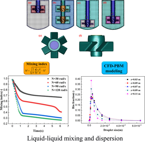
Liquid–liquid mixings in stirred tanks are commonly found in many industries. In this study, we performed computational fluid dynamics (CFD) modeling and simulation to investigate the liquid–liquid mixing behavior. Furthermore, the population balance model (PBM) was used to characterize the droplet size distribution. The PBM model parameters were calibrated using the experimental data of droplet sizes at different agitation speeds. Additionally, we employed the steady-state Sauter mean droplet size to validate the developed CFD–PBM coupled model at different dispersion phase holdups. Then, the validated CFD–PBM coupled model was employed to evaluate the role of impeller structural parameters on the liquid–liquid mixing efficiency based on a user-defined mixing index. It was found that the position of impellers significantly affects the mixing efficiency, and an increase in stirring speed and the number of impellers improved the mixing efficiency.
1. Introduction
Liquid–liquid mixing and dispersion phenomena are commonly found in many industrial processes, such as extraction, emulsification, polymerization, and wastewater treatment.1−5 In these processes, high liquid–liquid mixing rate and narrow droplet size distribution are required for excellent heat and mass transfer rates, which have remained challenging to obtain. Therefore, comprehensive knowledge of the hydrodynamic characteristics and droplet dispersion behavior of the liquid–liquid system has become necessary.
Liquid–liquid mixing and dispersion are performed in stirred tank reactors, where various internal structures make the process more complex. Many experiments have been performed to explore the characteristics of droplet size distribution in stirred tanks.6−9 Equally, many valuable correlations for droplet size have been proposed.10−12 It was found that the Sauter mean diameter and droplet size distribution shape highly depend on the impeller speed and continuous phase.13,14 Moreover, with the increase in impeller speed, the bimodal distribution profile in the aqueous continuous phase changed to unimodal distribution.14 Additionally, the dispersed phase holdup, dispersed phase viscosity, and continuous phase viscosity significantly affect the droplet size and size distribution.15−18 These attempts and efforts provide a systematic research method for liquid–liquid mixing and dispersion. However, it is expensive, time-consuming, and almost impossible to solely examine all key influencing factors via experiments.
As a supplementary approach, recently, computational fluid dynamics (CFD) coupled with population balance models (PBMs) has been widely used to characterize the liquid–liquid dispersion behavior.19−22 Several effective methods, such as the discrete method, quadrature method of moments (QMOM), and DQMOM, have been proposed to solve PBM. The discrete method directly computes the particle size distribution since the population is discretized into small size intervals. Thus, it is widely applied in modeling particle size distributions of gas–liquid and liquid–liquid systems. Rathore et al. investigated the gas dispersion characteristics and mass transfer coefficient in a gas–liquid stirred tank bioreactor.23 In their study, they employed the discrete method with 13 bins. Azargoshasb et al. proposed a CFD–PBM coupled model to investigate the bubbles’ Sauter mean diameter in a bioreactor.24 Eleven bin classes of arbitrary size were used to characterize the size distribution of the bubbles. Recently, Agahzamin and Pakzad developed an Eulerian–Eulerian model to evaluate the effect of the internals on gas holdup in a bubble column.25 Here, they employed the discrete method with 20 bins. Schütz et al. simulated the droplet size distribution in the water–diesel separation process in hydrocyclones for the liquid–liquid system.26 The droplet size was discretized into 19 bins. The calculated droplet size distributions showed good accordance with the experimental data. Vonka and Soos combined CFD and PBE to simulate droplet coalescence and breakup phenomena in a liquid–liquid stirred tank.27 They used QMOM to solve PBEs and predicted the dependency of the mean droplet size on impeller tip speed. Naeeni and Pakzad investigated the water-in-crude oil dispersions in a stirred tank.8 They solved the population balance equations using the discrete method with 20 bins. Their results show that an increase in agitation speed decreases the Sauter mean diameter. Furthermore, higher oil volume fractions result in a wider droplet size distribution, while increasing oil phase viscosity leads to a narrower droplet size distribution. Nonetheless, further investigations on mixing hydrodynamics for the liquid–liquid system are still required, particularly for considering the influence of complex impeller structural parameters.
In this study, we employed a CFD–PBM coupled model to evaluate the liquid–liquid mixing efficiency in stirred tanks. The simulation results were validated with the experimental data using Sauter’s mean size. Based on the validated model, the effects of stirring speed and the position and number of impellers on liquid–liquid mixing efficiency were investigated by a user-defined mixing index. This study gave a comprehensive understanding of the role of impeller structural parameters on liquid–liquid mixing characteristics in the stirred tank.
2. CFD–PBM Coupled Model Development
The CFD–PBM coupled model was developed and solved to obtain comprehensive flow field information on the liquid–liquid dispersion in stirred tanks. The CFD model includes a continuity equation, momentum equation, drag model, and turbulent model. The PBM model considers the breakage and coalescence effects of the droplets. The detailed model equations are given in the following.
2.1. CFD Model
The continuity and momentum equations are given as
| 1 |
| 2 |
In eq 2,  is the stress tensor, including the viscous
and turbulent tensors.
is the stress tensor, including the viscous
and turbulent tensors.
| 3 |
where μeff,q denotes the effective viscosity, including molecular and eddy viscosities, which are obtained by solving the RNG k–ε turbulent model.
| 4 |
| 5 |
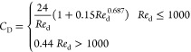
In eq 2, F is the combination of drag, buoyancy, gravity, lift, and virtual mass forces. The Schiller and Naumann drag model was used in this study and is given by28
 |
6 |
| 7 |
For the gravity and buoyancy forces, they can be combined and defined as
| 8 |
Besides, the lift and virtual mass forces were neglected in this study. This simplification is reasonable because the density ratio of the dispersion and continuous phases is close to one and the droplet size is small.29
2.2. PBM Model
For the liquid–liquid dispersion system, the droplet size distribution is fundamentally determined by the droplet coalescence and breakage phenomena. When the nucleation and growth rates are ignored, the population balance equation is written as a volume fraction of particle size i
| 9 |
where ρ is the density of the secondary phase and αi is the volume fraction of particle size i. BB and BC denote droplet birth, while DB and DC denote droplet death due to breakage and coalescence, respectively. In this study, we used the discrete method proposed by Hounslow et al. and Ramkrishna to model the droplet size distribution.30,31 Each droplet size interval is assumed as an independent Eulerian phase.26 Thus, it can be tracked to obtain the droplet size distribution. The droplet birth and death rates are defined as
 |
10 |
| 11 |
| 12 |
| 13 |
where the term ΩB(υi, υK) is the breakage rate of a droplet from size υi to size υK and the term Ωag(υi, υj) is the coalescence rate of a drop with sizes of υi and υj. To solve eq 9, breakage and coalescence source terms are required beforehand. Various models of breakage and coalescence phenomena have been reported in the literature.32−36 Here, breakage and coalescences of droplets were modeled using the Coulaloglou and Tavlarides model,37 which is widely employed to describe drop breakage and coalescence in turbulently agitated liquid–liquid dispersion. The equations for breakage and coalescence functions are defined as eqs 14 and 15, respectively
| 14 |
 |
15 |
Additionally, the daughter droplet distribution function is also required for calculating the droplet size distribution. A detailed discussion about the daughter distribution functions can be found in ref (38). In this study, we used the parabolic probability density function of droplets as follows
| 16 |
The volume fraction of each droplet size interval was solved by the discrete method. Therefore, the droplet size distribution function can be defined as follows
| 17 |
where α(i) is the volume fraction of bin i. Then, the mean droplet size can be defined as follows
| 18 |
The variance can be estimated as follows
| 19 |
A lower variance value indicates a narrow droplet size distribution.
2.3. Simulation Method
This study investigates the dispersion of methyl methacrylate into the water in stirred tank reactors, which have stationary and rotating zones involving impeller blades. The detailed reactor structures can be seen in Roudsari et al.’s work.39 The volume fraction of methyl methacrylate was varied from 20 to 50% (i.e., 20, 30, 40, and 50%). Four levels of impeller speed 30, 60, 90, and 120 rad/s were modeled.
The multiple reference frame method was used to model impeller motion under steady-state conditions,23,40−43 and the sliding mesh method was adopted under transient conditions for more accurate simulation results.44,45 The enhanced wall functions were employed to model the near-wall regions. The developed three-dimensional (3D) CFD–PBM coupled model was solved in ANSYS FLUENT with double-precision mode. Pressure and velocity were coupled using a SIMPLE algorithm. Furthermore, the volume fraction was discretized using a QUICK scheme, and the rest of the equations were discretized using the second-order upwind method. The PBM equations were solved using the discrete method that discretizes the droplet population into 15 bins. For the steady-state simulation, we checked the residual of continuity, momentum, volume fraction, turbulent kinetic energy, turbulent dissipation rate, and bin fraction equations. The converged solution was obtained when the residuals were below 1 × 10⁻⁴. For the unsteady state simulation, the time step was 0.001 s. All CFD simulations were executed on a 3.3 GHz Intel 1 CPU (10 cores) with 128 GB of RAM.
3. Results and Discussion
3.1. Mesh Independence Study
Grid resolution plays a significant role in determining the simulation results for the stirred tank reactor because of the large gradient of flow variables. In this study, we focused on refining the grid in the rotation area and close to the wall. Thus, we obtained the stirred tank reactor models with different grid resolutions: N = 1,052,968, N = 1,789,814, N = 2,664,451, and N = 3,265,367.
In this section, we performed CFD simulations to investigate the influence of grid resolution on the velocity and droplet size distribution when the dispersion phase holdup was 0.2 and impeller speed was 120 rad/s. Generally, we observed a significant spatial distribution of velocity in the stirred tank with high impeller speed. Therefore, two typical cross sections, one was the plane including the impeller (z = 0.05 m) and the other was below the impeller (z = 0.036 m), were selected and used to evaluate the variation trend of the velocity with the increase in the grid resolution. In Figure 1A,B, the velocity distribution is almost symmetric. Results show that the predicted velocity was insensitive to grid resolution when the number of cells exceeded one million. Additionally, there was a large velocity gradient near the wall, indicating that the grid resolution was enough to capture the detailed flow structures. Furthermore, the turbulence characteristics significantly influenced the droplet size distribution. Also, the effect of grid resolution on the droplet size distribution was investigated (see Figure 1C,D). Although significant differences were observed in the droplet size distribution at different locations of the stirred tank reactor, the droplet size distributions were relatively the same when the number of cells exceeded one million. From eqs 14 and 15, the same droplet size distribution at different grid resolutions means that the predicted turbulent dissipation rate is independent of the grid resolution.
Figure 1.

Mesh independence analysis: the effect of grid resolution on the velocity and droplet size distribution. (A, C) z = 0.05 m; (B, D) z = 0.036 m. (Simulation conditions: the dispersion phase holdup is 0.2 and impeller speed is 120 rad/s).
As discussed above, sufficient grid resolution did not change the velocity and droplet size distribution. In this study, we used the grid accuracy of N = 2664451 for the CFD simulation in the following.
3.2. CFD–PBM Model Validation
Before the CFD–PBM coupled model was applied to investigate the mixing and droplet size distribution characteristics in liquid–liquid stirred tanks, the model calibration and validation were inherently required. Here, the model parameters that required calibration mainly came from breakage and coalescence functions. Coulaloglou and Tavlarides found that the estimated breakage/coalescence frequency parameters were different when fitting different experimental data.37 This is because these parameters depend on the reactor structures, which significantly affect the turbulent dissipation rate. Many researchers have found different model parameters for various liquid–liquid systems.46−49
Previously, Jahanzad et al. studied the droplet size of a methyl methacrylate–water dispersion system.50 To determine the mechanisms affecting the droplet size, they investigated the dispersion of methyl methacrylate into water under two extreme stabilizer concentrations at different impeller speeds. They confirmed that the drops are sufficiently stable against coalescence at high stabilizer concentration, and the droplet size is determined only using the breakage effect. However, the detailed stirred tank reactor structures are unclear for us. Therefore, their experimental data were first employed to calibrate the developed CFD–PBM coupled model, which was then employed to investigate the mixing and dispersion characteristics in a given liquid–liquid stirred tank reactor.
Correspondingly, two simulation cases were performed: one considers both breakage and coalescence effects and the other only the breakage effect. Notably, only the steady-state Sauter mean diameters were calculated in this section because the unsteady state simulations were time-consuming. Generally, breakage/coalescence efficiency and frequency parameters needed to be calibrated. As discussed by Coulaloglou and Tavlarides, the roles of breakage/coalescence frequency parameters were more prominent, and therefore, the breakage frequency parameter and coalescence frequency parameter were calibrated in turn according to the reported experimental data. The model calibrations were performed to minimize the objective function, which is defined as
| 20 |
where dmod,i and dexp,i are the model and experimental predictions, respectively. The calibration values of the breakage and coalescence frequency were 1.2 and 0.0008, respectively. The used breakage and coalescence efficiency parameters were 0.08 and 2 × 10¹³, respectively.
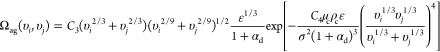
In Figure 2, the Sauter mean diameter is plotted against the agitation speed. Here, the Sauter mean diameter first decreased rapidly with the increasing agitation speed, meaning that the breakage effect was dominant at this stage. However, when the agitation speed exceeded a certain critical value (about 80 rad/s), a decreasing trend of the droplet size with respect to the increase of agitation speed was obtained. According to eq 14, the breakup resistance of small droplets was large and tends to coalesce. In this study, when only the breakage effect was considered, the droplet size decreased to 20 μm at an agitation speed of 120 rad/s. When both breakage and coalescence effects were considered, the steady-state Sauter mean droplet size showed a significant increase. However, the changing trend of the droplet size with agitation speed remained consistent. For the CFD simulation, the steady-state Sauter mean droplet size was obtained at different agitation speeds ranging from 20–120 rad/s.
Figure 2.
Steady-state Sauter mean droplet size vs agitation speed: experimental data and CFD simulation results.
Generally, a good similarity between the CFD simulation and experimental data was observed in the calibration step. With different agitation speeds, the root-mean-square error was obtained as 8.0 and 6.5 μm, indicating it was a good fit. Further validations will be performed by investigating the effect of dispersion phase holdup on droplet size.
Figure 3 displays a comparison of CFD simulation results and experimental data for the steady-state Sauter mean droplet size at different dispersion phase holdups. Here, the experimental data were reported by Jahanzad et al., who investigated the dispersions of methyl methacrylate at different volume fractions at an agitation speed of 300 rpm.50 We observed a linear relationship between the Sauter mean droplet size and dispersed phase holdup. An increase in the volume fraction dampens the turbulence intensity and increases the collision frequency. Therefore, the mean drop size experiences an increase. The following general form has been employed to predict the effect of dispersed phase holdup51−53
| 21 |
where d32, DI, ϕd, and We are the Sauter mean droplet size, impeller diameter, dispersed phase holdup, and Weber number, respectively. Here, the calibrated CFD–PBM coupled model shows good prediction performance. Therefore, further investigation of the dispersion characteristics of droplets can be expected based on the proposed CFD–PBM coupled model.
Figure 3.
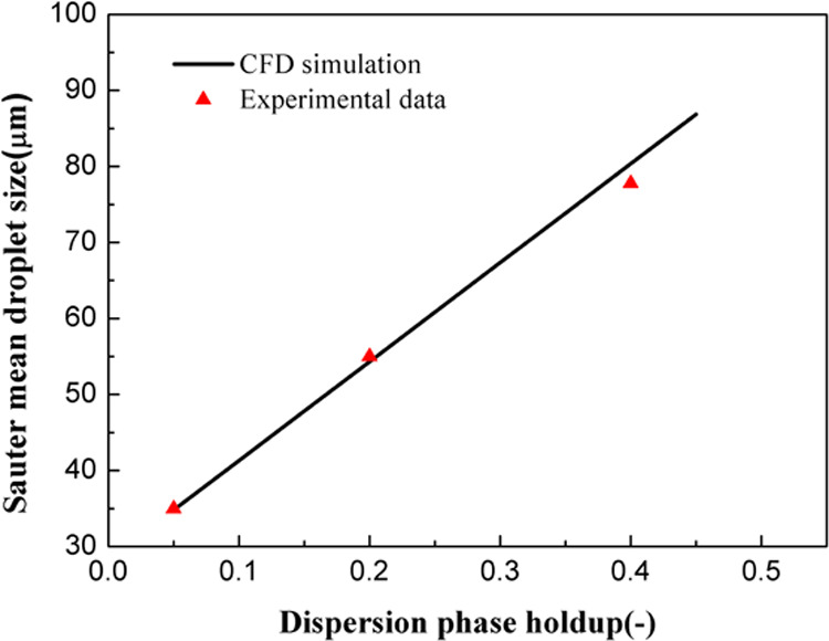
Comparison of the experimental data and CFD simulation results according to the steady-state Sauter mean droplet size at different dispersed phase holdups.
In addition to the Sauter mean droplet size, the droplet size distribution is also one of the most important evaluation indexes for the liquid–liquid dispersion system. Figure 4 displays the droplet size distribution at different impeller speeds. As discussed above, the mean droplet size decreases with increased impeller speed. Equations 14 and 15 show that higher breakage and coalescence rates were observed at higher impeller speed. However, the breakage rate was more sensitive than the coalescence rate when the impeller speed increased, thereby decreasing the droplet size. Additionally, the variance also decreased from 1.27 × 10⁻⁸ to 1.44 × 10⁻⁹ with an increase in the impeller speed from 60–120 rad/s. This indicated that a wider droplet size distribution profile could be achieved at a lower impeller speed.
Figure 4.

Effect of impeller speed on droplet size distribution.
3.3. Liquid–Liquid Mixing Behavior
We characterized the liquid–liquid mixing and separation behavior quantitatively by a user-defined mixing index defined as
| 22 |
where N is the total number of grids, α is the local phase holdup, and α̅ is the average phase holdup. At the beginning time, the dispersed phase was patched at the top of the stirred tank; then, the mixing index was calculated and recorded with flow time. Since the continuous phase and the dispersed phase were completely separated at the initial time, the mixing index was equal to 1.
First, we investigated the effect of stirring speed on liquid–liquid mixing efficiency. Figure 5 shows the time evolution of the mixing index at different stirring speeds. From eq 22, the mixing index will experience a decrease when the liquid–liquid mixing is improved. For ideal mixing, the mixing index equals zero. In this study, two mixing stages were observed, as shown in Figure 5. In the first stage, the mixing index was sensitive to the mixing time (t < 1.5 s). The rotation of the impeller generated negative pressure, causing the dispersed phase to sink along the stirring shaft. When the dispersed phase reached the impeller zone, intense two-phase mixing occurred. Therefore, the mixing index decreased significantly in this stage. In the second stage, the liquid–liquid dispersion and mixing achieved an equilibrium, and the mixing index remained nearly constant.
Figure 5.
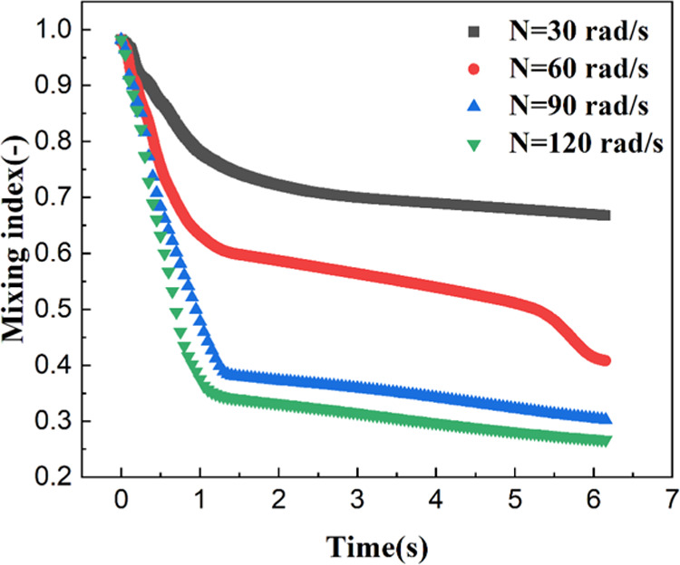
Time evolution of the mixing index at different agitation speeds.
The higher agitation speed is responsible for the better mixing effect, and therefore, a small mixing index will be obtained. When the agitation speed was 30 rad/s, the equilibrium mixing index was 0.67, which deviated from the perfect mixing case. This is because there are some stagnant zones in the stirred tank. When the agitation speed increased to 120 rad/s, however, the mixing index could be as low as 0.27, which is very close to the perfect mixing. From Figure 5, it could be also concluded that when the agitation speed was higher than 90 rad/s, the mixing index became independent on agitation speed.
More details about liquid–liquid mixing can be also seen in the time evolution of the contour of dispersed phase holdup at different agitation speeds. As shown in Figure 6, the dispersion phase tended to adhere to the wall of the stirring shaft. Although the agitation speed was as high as 120 rad/s, this adhesion effect also existed. For the continuous phase, however, it tended to accumulate at the bottom of the impeller. This phenomenon was determined by the impeller structure. The fluid velocity almost equals zero at the bottom of the impeller. The density of the continuous phase is greater than that of the dispersed phase, leading to the accumulation of the continuous phase at the bottom of the impeller.
Figure 6.
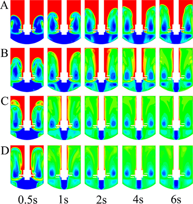
Time evolution of the contour of dispersed phase holdup at different agitation speeds. (A: 30 rad/s; B: 60 rad/s; C: 90 rad/s; D: 120 rad/s).
From Figure 6, there were four main vortices in the stirred tank under low agitation speed (i.e., 30 and 60 rad/s). When the agitation speed was higher than 90 rad/s, as could be seen, there were only two vortices in the stirred tank. This implied that the position of the impeller significantly affected the liquid–liquid mixing effect. Generally, promoting communication between the fluids located at different vortices can significantly improve the mixing efficiency.
As already discussed above, the position of the impeller significantly affected the liquid–liquid mixing effect because the fluid velocity almost equaled to zero at a position away from the impeller. For the stirred tank reactor, the number of impellers also plays an important role in determining the mixing effect. Figure 7 displays the detailed impeller structures in the stirred tank reactor. Taking the standard stirred tank reactor as reference, the effects of the position and number of impellers on liquid–liquid mixing efficiency were investigated when the agitation speed was 60 rad/s. In this work, a low stirring speed was used as already observed above that the liquid–liquid mixing was poor.
Figure 7.

Detailed impeller structures in the stirred tank reactor: (a) single impeller located at the top of the reactor; (b) double impeller; (c) single impeller located at the bottom of the reactor; (d) reference impeller; (e, f) structure of the impeller.
Figure 8 displays the effect of the position and number of impellers on the time evolution of the contour of dispersed phase holdup. As already discussed above, there was a stagnant region at the bottom of the impeller. From Figure 8A, when the impeller was far away from the vessel bottom, the area of the stagnation region increased, indicating poor liquid–liquid mixing efficiency. We tried to decrease the distance from the impeller to the vessel bottom to explore its effect on liquid–liquid mixing. As can be seen in Figure 8C, although the stagnation region at the bottom of the impeller decreased, the stagnation region at the top of the stirred tank increased, and thus, the liquid–liquid mixing was still poor. Therefore, this study further investigated the effect of a double impeller on liquid–liquid mixing. From Figure 8B, not surprisingly, the liquid–liquid mixing effect had been significantly improved. When compared with the situation of a single impeller, the advantage of the double impeller was that it could weaken the internal circulation of a continuous phase, and thus promoting the mixing between the continuous phase and dispersed phase. Figure 9 displays time evolution of the mixing index at different structures of the impeller. The variation trend of the mixing index was consistent with the distribution of dispersed phase holdup, which was already discussed above. Therefore, we only discussed the effect of the single impeller and double impeller on liquid–liquid mixing. By comparing Figures 6B and 8B, it seemed that the mixing efficiency of the single impeller was better than that of the double impeller. Due to the complexity of the structure of a double impeller, many dispersed phases adhered to the wall, which was the main reason for its low mixing efficiency when compared with that of a single impeller at the same stirring speed. However, this may be not true for all situations. For a small stirred speed (i.e., 30 rad/s), the single impeller could not mix the liquid–liquid two phase well. Therefore, the structure of the double impeller may have its advantages at low stirring speed.
Figure 8.

Effect of the position and number of impellers on the time evolution of the contour of dispersed phase holdup when the stirring speed is 60 rad/s. (A: single impeller located at the top of the reactor; B: double impeller; C: single impeller located at the bottom of the reactor).
Figure 9.
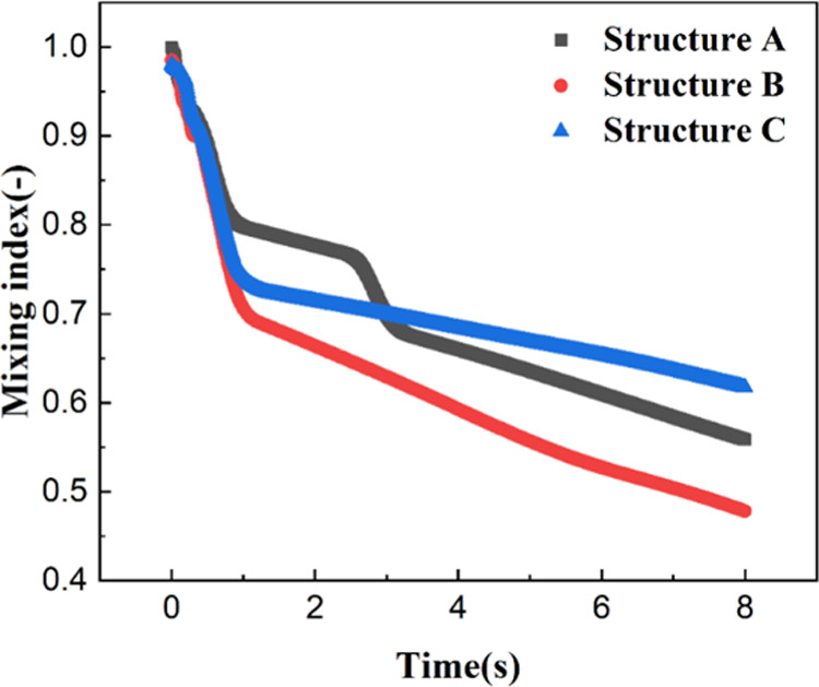
Time evolution of the mixing index at different structures of the impeller (structure A: single impeller located at the top of the reactor; structure B: double impeller; structure C: single impeller located at the bottom of the reactor).
4. Conclusions
In this study, we investigated the liquid–liquid mixing and dispersion behavior using the proposed CFD–PBM coupled modeling and simulation method. The experimental data of droplet sizes at different agitation speeds were employed to calibrate PBM model parameters. Then, we validated the proposed CFD–PBM coupled model using the steady-state Sauter mean droplet size at different dispersed phase holdups.
From the validated CFD–PBM coupled model, the spatial and temporal distribution characteristics of the droplet size were analyzed. The results showed that the variance decreased from 1.27 × 10⁻⁸ to 1.44 × 10⁻⁹ when the impeller speed increased from 60–120 rad/s. Furthermore, wider droplet size distribution profiles were achieved at a lower impeller speed. Moreover, the efficiency of the liquid–liquid mixing was quantitatively characterized using a user-defined mixing index. Generally, two mixing stages were observed. When the agitation speed increased from 30 to 120 rad/s, the mixing index decreased from 0.67 to 0.27. Then, the role of four impeller structural parameters on liquid–liquid mixing characteristics was investigated. For a single impeller, the poor liquid–liquid mixing efficiency was observed at positions away from the impeller, such as the top and bottom of the stirred tank. It was found that the double impeller could solve this problem, especially at a low stirring speed.
Acknowledgments
The authors are grateful to the National Natural Science Foundation of China (22108314); the Natural Science Foundation of Hunan Province (2021JJ40717); and the Center for High Performance Computing, Shanghai Jiao Tong University for financial support.
Glossary
Abbreviations
- BB
birth rate of drops for breakage (1/(m3·s))
- BC
birth rate of drops for coalescence (1/(m3·s))
- CD
drag coefficient
- C1ε,C2ε
coefficients in turbulence model
- d:
diameter of the drop (m)
- d32
diameter of the drop (m)
- DB
death rate of drops for breakage (1/(m3·s))
- Dc
death rate of drops for coalescence (1/(m3·s))
- g
gravitational acceleration (m·s–2)
- κ
turbulence kinetic energy, (m2·s–2)
- P
pressure (Pa)
- Re
Reynolds number
Glossary
Greek Letters
- ρ
density (kg·m–3)
- μ
viscosity (Pa·s)
- α
volume fraction
- ΩB
breakage rate of a droplet
- Ωag
coalescence rate of a drop
- τ
stress tensor (Pa)
- ε
turbulence dissipation rate (s–1)
- σ
variance (s)
The authors declare no competing financial interest.
References
- Yu X.; Zhou H.; Jing S.; Lan W.; Li S. CFD–PBM simulation of two-phase flow in a pulsed disc and doughnut column with directly measured breakup kernel functions. Chem. Eng. Sci. 2019, 201, 349–361. 10.1016/j.ces.2019.03.010. [DOI] [Google Scholar]
- Vikhansky A. CFD modelling of turbulent liquid–liquid dispersion in a static mixer. Chem. Eng. Process. 2020, 149, 107840 10.1016/j.cep.2020.107840. [DOI] [Google Scholar]
- Xie L.; Liu Q.; Luo Z.-H. A multiscale CFD–PBM coupled model for the kinetics and liquid–liquid dispersion behavior in a suspension polymerization stirred tank. Chem. Eng. Res. Des. 2018, 130, 1–17. 10.1016/j.cherd.2017.11.045. [DOI] [Google Scholar]
- Wang Z.; Li T.; Wang F.; Guan L.; Zhang R. Numerical simulation of polymer dispersion systems for polymer injection on offshore platforms. ACS omega 2020, 5, 20343–20352. 10.1021/acsomega.0c02307. [DOI] [PMC free article] [PubMed] [Google Scholar]
- Nazar M.; Shah M. U. H.; Ahmad A.; Yahya W. Z. N.; Goto M.; Moniruzzaman M. Ionic liquid and tween-80 mixture as an effective dispersant for oil spills: Toxicity, biodegradability, and optimization. ACS omega 2022, 7, 15751–15759. 10.1021/acsomega.2c00752. [DOI] [PMC free article] [PubMed] [Google Scholar]
- Angle C. W.; Hamza H. A. Predicting the sizes of toluene-diluted heavy oil emulsions in turbulent flow part 2: Hinze–kolmogorov based model adapted for increased oil fractions and energy dissipation in a stirred tank. Chem. Eng. Sci. 2006, 61, 7325–7335. 10.1016/j.ces.2006.01.014. [DOI] [Google Scholar]
- EL-Hamouz A.; Cooke M.; Kowalski A.; Sharratt P. Dispersion of silicone oil in water surfactant solution: Effect of impeller speed, oil viscosity and addition point on drop size distribution. Chem. Eng. Process. 2009, 48, 633–642. 10.1016/j.cep.2008.07.008. [DOI] [Google Scholar]
- Khajeh Naeeni S.; Pakzad L. Experimental and numerical investigation on mixing of dilute oil in water dispersions in a stirred tank. Chem. Eng. Res. Des. 2019, 147, 493–509. 10.1016/j.cherd.2019.05.024. [DOI] [Google Scholar]
- Mirshekari F.; Pakzad L.; Fatehi P. An investigation on the stability of the hazelnut oil-water emulsion. J. Dispersion Sci. Technol. 2020, 41, 929–940. 10.1080/01932691.2019.1614459. [DOI] [Google Scholar]
- Brown D. E.; Pitt K. Drop size distribution of stirred non-coalescing liquid-liquid system. Chem. Eng. Sci. 1972, 27, 577–583. 10.1016/0009-2509(72)87013-1. [DOI] [Google Scholar]
- Calabrese R. V.; Chang T. P. K.; Dang P. T. Drop breakup in turbulent stirred-tank contactors. Part i: Effect of dispersed-phase viscosity. AIChE J. 1986, 32, 657–666. 10.1002/aic.690320416. [DOI] [Google Scholar]
- Lemenand T.; Della Valle D.; Zellouf Y.; Peerhossaini H. Droplets formation in turbulent mixing of two immiscible fluids in a new type of static mixer. Int. J. Multiphase Flow 2003, 29, 813–840. 10.1016/S0301-9322(03)00032-6. [DOI] [Google Scholar]
- Zhou G.; Kresta S. M. Correlation of mean drop size and minimum drop size with the turbulence energy dissipation and the flow in an agitated tank. Chem. Eng. Sci. 1998, 53, 2063–2079. 10.1016/S0009-2509(97)00438-7. [DOI] [Google Scholar]
- Pacek A. W.; Chamsart S.; Nienow A. W.; Bakker A. The influence of impeller type on mean drop size and drop size distribution in an agitated vessel. Chem. Eng. Sci. 1999, 54, 4211–4222. 10.1016/S0009-2509(99)00156-6. [DOI] [Google Scholar]
- Lovick J.; Mouza A. A.; Paras S. V.; Lye G. J.; Angeli P. Drop size distribution in highly concentrated liquid–liquid dispersions using a light back scattering method. J. Chem. Technol. Biotechnol. 2005, 80, 545–552. 10.1002/jctb.1205. [DOI] [Google Scholar]
- Boxall J. A.; Koh C. A.; Sloan E. D.; Sum A. K.; Wu D. T. Measurement and calibration of droplet size distributions in water-in-oil emulsions by particle video microscope and a focused beam reflectance method. Ind. Eng. Chem. Res. 2010, 49, 1412–1418. 10.1021/ie901228e. [DOI] [Google Scholar]
- Vladisavljević G. T.; Kobayashi I.; Nakajima M. Effect of dispersed phase viscosity on maximum droplet generation frequency in microchannel emulsification using asymmetric straight-through channels. Microfluid. Nanofluid. 2011, 10, 1199–1209. 10.1007/s10404-010-0750-9. [DOI] [Google Scholar]
- De Hert S. C.; Rodgers T. L. On the effect of dispersed phase viscosity and mean residence time on the droplet size distribution for high-shear mixers. Chem. Eng. Sci. 2017, 172, 423–433. 10.1016/j.ces.2017.07.002. [DOI] [Google Scholar]
- Guo X.; Zhao Q.; Zhang T.; Zhang Z.; Zhu S. Liquid–liquid flow in a continuous stirring settler: CFD-PBM simulation and experimental verification. JOM 2019, 71, 1650–1659. 10.1007/s11837-019-03396-w. [DOI] [Google Scholar]
- Yu X.; Zhou H.; Jing S.; Lan W.; Li S. Augmented CFD–PBM simulation of liquid–liquid two-phase flows in liquid extraction columns with wettable internal plates. Ind. Eng. Chem. Res. 2020, 59, 8436–8446. 10.1021/acs.iecr.0c01476. [DOI] [Google Scholar]
- Zhou H.; Yu X.; Wang B.; Jing S.; Lan W.; Li S. CFD–PBM simulation of liquid–liquid dispersions in a pump-mixer. Ind. Eng. Chem. Res. 2021, 60, 1926–1938. 10.1021/acs.iecr.0c05745. [DOI] [Google Scholar]
- Qin C.; Chen C.; Xiao Q.; Yang N.; Yuan C.; Kunkelmann C.; Cetinkaya M.; Muelheims K. CFD-PBM simulation of droplets size distribution in rotor-stator mixing devices. Chem. Eng. Sci. 2016, 155, 16–26. 10.1016/j.ces.2016.07.034. [DOI] [Google Scholar]
- Rathore A. S.; Sharma C.; Persad Use of computational fluid dynamics as a tool for establishing process design space for mixing in a bioreactor. Biotechnol. Progr. 2012, 28, 382–391. 10.1002/btpr.745. [DOI] [PubMed] [Google Scholar]
- Azargoshasb H.; Mousavi S. M.; Jamialahmadi O.; Shojaosadati S. A.; Mousavi S. B. Experiments and a three-phase computational fluid dynamics (CFD) simulation coupled with population balance equations of a stirred tank bioreactor for high cell density cultivation. Can. J. Chem. Eng. 2016, 94, 20–32. 10.1002/cjce.22352. [DOI] [Google Scholar]
- Agahzamin S.; Pakzad L. A comprehensive cfd study on the effect of dense vertical internals on the hydrodynamics and population balance model in bubble columns. Chem. Eng. Sci. 2019, 193, 421–435. 10.1016/j.ces.2018.08.052. [DOI] [Google Scholar]
- Schütz S.; Gorbach G.; Piesche M. Modeling fluid behavior and droplet interactions during liquid–liquid separation in hydrocyclones. Chem. Eng. Sci. 2009, 64, 3935–3952. 10.1016/j.ces.2009.04.046. [DOI] [Google Scholar]
- Vonka M.; Soos M. Characterization of liquid-liquid dispersions with variable viscosity by coupled computational fluid dynamics and population balances. AIChE J. 2015, 61, 2403–2414. 10.1002/aic.14831. [DOI] [Google Scholar]
- Schiller L. A drag coefficient correlation. Zeit. Ver. Deutsch. Ing. 1933, 77, 318–320. [Google Scholar]
- Naeeni S. K.; Pakzad L. Droplet size distribution and mixing hydrodynamics in a liquid–liquid stirred tank by CFD modeling. Int. J. Multiphase Flow 2019, 120, 103100 10.1016/j.ijmultiphaseflow.2019.103100. [DOI] [Google Scholar]
- Hounslow M. J.; Ryall R. L.; Marshall V. R. A discretized population balance for nucleation, growth, and aggregation. AIChE J. 1988, 34, 1821–1832. 10.1002/aic.690341108. [DOI] [Google Scholar]
- Ramkrishna D. The status of population balances. Rev. Chem. Eng. 1985, 3, 49–95. 10.1515/REVCE.1985.3.1.49. [DOI] [Google Scholar]
- Nambiar D. K. R.; Kumar R.; Das T. R.; Gandhi K. S. A new model for the breakage frequency of drops in turbulent stirred dispersions. Chem. Eng. Sci. 1992, 47, 2989–3002. 10.1016/0009-2509(92)87001-7. [DOI] [Google Scholar]
- Alopaeus V.; Koskinen J.; Keskinen K. I. Simulation of the population balances for liquid–liquid systems in a nonideal stirred tank. Part 1 description and qualitative validation of the model. Chem. Eng. Sci. 1999, 54, 5887–5899. 10.1016/S0009-2509(99)00170-0. [DOI] [Google Scholar]
- Alopaeus V.; Koskinen J.; Keskinen K. I.; Majander J. Simulation of the population balances for liquid–liquid systems in a nonideal stirred tank. Part 2-parameter fitting and the use of the multiblock model for dense dispersions. Chem. Eng. Sci. 2002, 57, 1815–1825. 10.1016/S0009-2509(02)00067-2. [DOI] [Google Scholar]
- Luo H.; Svendsen H. F. Theoretical model for drop and bubble breakup in turbulent dispersions. AIChE J. 1996, 42, 1225–1233. 10.1002/aic.690420505. [DOI] [Google Scholar]
- Ghadiri M.; Zhang Z. Impact attrition of particulate solids. Part 1: A theoretical model of chipping. Chem. Eng. Sci. 2002, 57, 3659–3669. 10.1016/S0009-2509(02)00240-3. [DOI] [Google Scholar]
- Coulaloglou C. A.; Tavlarides L. L. Description of interaction processes in agitated liquid-liquid dispersions. Chem. Eng. Sci. 1977, 32, 1289–1297. 10.1016/0009-2509(77)85023-9. [DOI] [Google Scholar]
- Liao Y.; Lucas D. A literature review of theoretical models for drop and bubble breakup in turbulent dispersions. Chem. Eng. Sci. 2009, 64, 3389–3406. 10.1016/j.ces.2009.04.026. [DOI] [Google Scholar]
- Roudsari S. F.; Ein-Mozaffari F.; Dhib R. Use of CFD in modeling mma solution polymerization in a cstr. Chem. Eng. J. 2013, 219, 429–442. 10.1016/j.cej.2012.12.049. [DOI] [Google Scholar]
- Pakzad L.; Ein-Mozaffari F.; Chan P. Using electrical resistance tomography and computational fluid dynamics modeling to study the formation of cavern in the mixing of pseudoplastic fluids possessing yield stress. Chem. Eng. Sci. 2008, 63, 2508–2522. 10.1016/j.ces.2008.02.009. [DOI] [Google Scholar]
- Hosseini S.; Patel D.; Ein-Mozaffari F.; Mehrvar M. Study of solid– liquid mixing in agitated tanks through computational fluid dynamics modeling. Ind. Eng. Chem. Res. 2010, 49, 4426–4435. 10.1021/ie901130z. [DOI] [Google Scholar]
- Fan L.; Xu N.; Wang Z.; Shi H. Pda experiments and CFD simulation of a lab-scale oxidation ditch with surface aerators. Chem. Eng. Res. Des. 2010, 88, 23–33. 10.1016/j.cherd.2009.07.013. [DOI] [Google Scholar]
- Roudsari S. F.; Turcotte G.; Dhib R.; Ein-Mozaffari F. CFD modeling of the mixing of water in oil emulsions. Comput. Chem. Eng. 2012, 45, 124–136. 10.1016/j.compchemeng.2012.06.013. [DOI] [Google Scholar]
- Wutz J.; Lapin A.; Siebler F.; Schäfer J. E.; Wucherpfennig T.; Berger M.; Takors R. Predictability of kla in stirred tank reactors under multiple operating conditions using an euler–lagrange approach. Eng. Life Sci. 2016, 16, 633–642. 10.1002/elsc.201500135. [DOI] [Google Scholar]
- Kazemzadeh A.; Ein-Mozaffari F.; Lohi A.; Pakzad L. Investigation of hydrodynamic performances of coaxial mixers in agitation of yield-pseudoplasitc fluids: Single and double central impellers in combination with the anchor. Chem. Eng. J. 2016, 294, 417–430. 10.1016/j.cej.2016.03.010. [DOI] [Google Scholar]
- Bapat P. M.; Tavlarides L. L. Mass transfer in a liquid-liquid cfstr. AIChE J. 1985, 31, 659–666. 10.1002/aic.690310416. [DOI] [Google Scholar]
- Ross S. L.; Verhoff F. H.; Curl R. L. Droplet breakage and coalescence processes in an agitated dispersion. 2. Measurement and interpretation of mixing experiments. Ind. Eng. Chem. Fundam. 1978, 17, 101–108. 10.1021/i160066a006. [DOI] [Google Scholar]
- Ribeiro L. M.; Regueiras P. F. R.; Guimaraes M. M. L.; Madureira C. M. N.; Cruz-Pinto J. J. C. The dynamic behaviour of liquid-liquid agitated dispersions—i. The hydrodynamics. Comput. Chem. Eng. 1995, 19, 333–343. 10.1016/0098-1354(94)00054-R. [DOI] [Google Scholar]
- Azizi F.; Al Taweel A. M. Turbulently flowing liquid–liquid dispersions. Part i: Drop breakage and coalescence. Chem. Eng. J. 2011, 166, 715–725. 10.1016/j.cej.2010.11.050. [DOI] [Google Scholar]
- Jahanzad F.; Sajjadi S.; Brooks B. W. Comparative study of particle size in suspension polymerization and corresponding monomer– water dispersion. Ind. Eng. Chem. Res. 2005, 44, 4112–4119. 10.1021/ie048827f. [DOI] [Google Scholar]
- Lagisetty J. S.; Das P. K.; Kumar R.; Gandhi K. S. Breakage of viscous and non-newtonian drops in stirred dispersions. Chem. Eng. Sci. 1986, 41, 65–72. 10.1016/0009-2509(86)85198-3. [DOI] [Google Scholar]
- Coulaloglou C. A.; Tavlarides L. L. Drop size distributions and coalescence frequencies of liquid-liquid dispersions in flow vessels. AIChE J. 1976, 22, 289–297. 10.1002/aic.690220211. [DOI] [Google Scholar]
- Mlynek Y.; Resnick W. Drop sizes in an agitated liquid-liquid system. AIChE J. 1972, 18, 122–127. 10.1002/aic.690180122. [DOI] [Google Scholar]