

Abstract
Transport phenomena in microfluidic chips are induced by electric fields and electrolyte concentrations. Liquid flows are often affected by ionic currents driven by electric fields in narrow channels, which are applied in microelectromechanical systems, microreactors, lab-on-a-chip, and so forth. Even though numerical studies to evaluate those local fields have been reported, measurement methods seem to be under construction. To deeply understand the dynamics of ions at the microscale, measurement techniques are necessary to be developed. In this study, we propose a novel method to directly measure electrical potential differences in liquids, local electric fields, and electrical conductivities, using a glass microelectrode. Scanning an electrolyte solution, for example, KCl solutions, with a 1 μm tip under constant ionic current conditions, a potential difference in liquids is locally measured with a micrometer-scale resolution. The conductivity of KCl solutions ranging from 0.56 to 100 mM is evaluated from electric fields locally measured, and errors are within 5% compared with the reference values. It is found that the present method enables us to directly measure local electric fields under constant current and that the electrical conductivity is quantitatively evaluated. Furthermore, it is suggested that the present method is available for various electrical analyses without calibration procedures before measurements.
Introduction
In recent decades, various functions of microfluidic devices have attracted significant attention. Focusing on transport phenomena in fluids, several applications have been proposed for microelectromechanical systems (MEMS) and micro-total analysis systems (μ-TAS),1,2 for example, flow sensors,3,4 micromixers,5 and microreactors.6 Microscale convective heat transfer7,8 and mass transport phenomena9,10 have also been investigated. A small amount of fluid is effective to express novel functions at micro- and nanoscales. In micro- and nanofluidic channels that are filled with electrolyte solutions, electric double layers are formed by highly concentrated counterion near the channel surface and induce an electroosmotic flow (EOF) under external electric fields.11−14 EOFs are also known to be generated in ion-exchange materials in which electrically charged functional groups are fixed, as well as in artificially manufactured fluidic channels.15,16 In highly polarized conditions, liquid flows are driven by ion transport in strong electric fields. We also reported that this kind of phenomena could be observed in the macroscopic liquid phase, which is known as electrohydrodynamic flows.15,17 On the other hand, we do not have conventional methods to evaluate electrolyte concentrations and electric fields in such small spaces.
In a previous study, it was reported that the transport of biomacromolecules, for example, deoxyribonucleic acid, confined in a nanochannel could be effectively transformed between stretched and compressed shapes.18 We found that the terminal velocity of the molecule confined in the nanochannel depended on the applied electric field, ion conductivity, and EOFs. The flow velocity was strongly influenced by the channel size, and the counterflow to the electrophoresis of a molecule caused to determine the conformation. It is usually known that the size difference between the test section and the other channels for liquid introduction is extremely large and that the electric field and flow velocity become stronger in the test section.19 Such a confined test section is crucial to attaining the high sensitivity of sensors. Therefore, the optimization of electric fields and electrolyte concentrations in the fluidic channels is an important issue. Experiments and numerical analyses were also performed focusing on the dumbbell-shaped fluidic channels20,21 and the tip of capillaries.22,23 We also experimentally and theoretically demonstrated transient responses of ionic current near the electrodes.24 On the other hand, there has been difficulty in determining boundary conditions at the electrode surfaces. Electrochemical reactions and the formation of electric double layers and diffusion layers are transiently developed, and this kind of responses usually takes a long period until the steady states.24 Therefore, the numerical studies may be limited to qualitative analysis. It is helpful for the numerical analyses if electric and flow fields in microfluidic channels are locally determined without the influence of the electrode surfaces.
In this study, we introduce a conceptual idea to evaluate the electrical conductivity and/or concentrations of electrolyte solutions by measuring a local electric field in a fluidic channel. Using a small test section placed in a vessel and a glass microelectrode, the electrical potential distribution is locally measured without being affected by the potential drop at the electrode surfaces and reservoirs. Herein, a glass microelectrode is used for a probe of electrical potential measurement in liquids. By using the glass capillary that is often used for the action potential measurement of biological cells, we tackle to measure local electric fields. The tip size of the microelectrode is 1 μm or less, and the spatial resolution is expected to be comparable to the tip size. The test section in a liquid vessel is well designed to maintain uniform electric fields.25 Using a motorized stage, the microelectrode is swept along the channel with a step varied from 20 to 200 μm. This direct measurement of local electric fields enables us to evaluate the conductivity or concentration without calibration. As a result, the conductivity of KCl standard solutions is accurately analyzed in the range of 1 to 100 mM. The present result will shed light on the measurement methods of small spaces like microfluidic channels that are inevitable for MEMS and μ-TAS. Based on the concept demonstrated in this study, further applications and optimization for individual systems are expected.
Experimental Methods
Electrical Measurement Setup
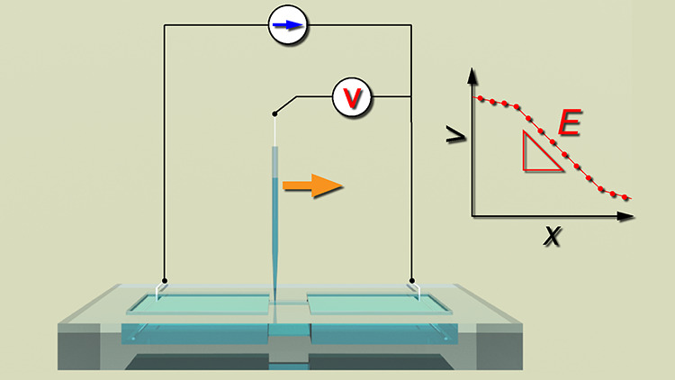
As shown in Figure 1, the experimental setup consists of a liquid vessel and an electrical measurement system. A test section placed between reservoirs is manufactured on an acrylic plate with a thickness of 3 mm, using a numerically controlled milling machine (KitMill CL200, Originalmind Inc., Okatani, Japan). As shown in Figure 2a, three types of the vessel structure are prepared: a test section 2.60 mm long, 0.96 mm wide, and 1.55 mm high and reservoirs 9.25 mm long, 9.25 mm wide, and 1.97 mm high; a test section 2.70 mm long, 1.05 mm wide, and 0.98 mm high and reservoirs 2.88 mm long, 9.85 mm wide, and 2.06 mm high; and a test section 2.82 mm long, 1.10 mm wide, and 2.01 mm high and reservoirs 9.93 mm long, 2.72 mm wide, and 2.10 mm high. Hereafter, these vessels are referred to as VT1, VT2, and VT3, respectively. The aspect ratios of the reservoirs and the test section are varied (see Table S2). The vessel is filled with a KCl standard solution of 0.56, 10, and 100 mM (Thermo Fisher Scientific, Inc., Singapore), and is settled on a hot plate (ND-1A, As One Corp., Osaka, Japan) with a sealing compound (KS650N-100, Shin-Etsu Chemical Co., Ltd., Tokyo, Japan) to maintain a liquid temperature at 303 K (30 °C). Using a galvanostat (EC-STAT-400, EC Frontier Co., Ltd., Kyoto, Japan), an electrical potential is locally measured in a solution under a constant current of 1 or 10 μA, where the working electrode (WE) and the counter electrode (CE) are settled in both ends of the reservoirs. A Ag–AgCl wire is used for the WE and CE, which is made of a Ag wire with a diameter of 0.3 mm (Nilaco Corp., Tokyo, Japan), being immersed in a sodium hypochlorite solution. The reference electrode (RE) also consists of a Ag–AgCl wire that is enclosed in a glass capillary filled with an electrolyte solution. Here, we use a KCl solution for the inner solution of the glass capillary, which is also called a glass microelectrode, as shown in Figure 2b. The concentration of the inner solution is properly prepared as mentioned later. The RE is clamped on the stage and dipped in the sample solution from the upper face of the liquid vessel (Figure 1). A potential difference between the WE and the RE is measured and recorded, sweeping the RE along the test section using a motorized stage (XMSG615, Suruga Seiki Co., Ltd., Shizuoka, Japan). The spatial resolution of the motorized stage manipulated by a stepping motor is 1 μm. The electrical potential is measured for 10 s with a sampling frequency of 10 Hz at each point with an interval of 200 μm. This distance is much larger than the tip of the glass capillary that is less than 1 μm as mentioned later. As a result, we can obtain the spatial distribution of the electrical potential difference in the solution. In other words, electrical potential distributions in liquids are visualized. In a narrow rectangular test section, the lines of electric force are highly concentrated, and the concentration of electrolytes is uniform at the center of solutions. Therefore, the electrical potential difference is proportional to the displacement along the test section, and the electric field is confirmed to be uniform. In such a condition, the current–voltage (I–V) characteristics is Ohmic, and the conductivity is obtained as a constant. In this study, the electrical measurement accuracy is evaluated using KCl standard solutions.
Figure 1.

Schematic illustration of the experimental setup for local electrical potential measurement.
Figure 2.

(a) Three types of vessel structures and dimensions used in experiments: VT1 (left), VT2 (center), and VT3 (right). (b) Photograph of a glass microelectrode for the RE, which is made of a glass tube heated and pulled using a glass tube puller.
Preparation for Glass Microelectrodes
A glass tube with an outer diameter of 1.5 mm (G-1.5, Narishige Co., Ltd., Tokyo, Japan) is ultrasonicated in 99.5% ethanol and pure water for 5 min each and is baked on a hot plate at 473 K (200 °C) for 5 min. After cleaning, it is pulled to form a glass capillary with desired outer diameters of 0.6 or 1 μm using a glass tube puller (PE-22, Narishige Co., Ltd., Tokyo, Japan) (Figure 2b). A Ag–AgCl wire with a diameter of 0.2 mm (Nilaco Corp., Tokyo, Japan) is settled in the glass capillary filled with a KCl solution, and this glass microelectrode is for the RE. As a first step, the concentration of the inner solution is set to be equal to the sample solution. To increase the impedance of the glass microelectrode, an agarose gel is filled in a 1 μm tip of the capillary. In this case, a 120 mg agar is stirred in a 100 mM KCl aqueous solution of 30 mL and is heated using an alcohol lamp to harden the gel by decreasing the temperature. The quantity of agar and the concentration of KCl solution are optimized to minimize errors in the electrical measurements.
Electrical Conductivity Analysis
Electrical potential distributions measured at each point during the glass microelectrode is moved along the test section are recorded as time series data. The data set is translated to a histogram, and then a multimodal distribution is obtained as a function of the potential difference. Peaks in each distribution, which consists of 100 data points, are separated from the continuous distribution. Then, the mean values of the separated unimodal distributions are evaluated within a 95% confidence interval. Next, they can be translated to a potential difference as a function of distance with a scanning step length of 200 μm. Calculating the numerical difference of the electrical potential distribution, an electric field E can be obtained at each position. Averaging the electric field in the test section, the mean value of E is used for the evaluation of conductivity (Supporting Information Figure S1). Herein, seven data points are used for the average. Associated with the cross-section area of the test section, the current density j is evaluated, and the conductivity σ is determined based on Ohm’s law: j = σE. In this study, it is clarified that the electrical potential difference is linearly changed, and the electric field is uniform in the test section. According to the Nernst–Planck and Poisson equations,24 it is clarified that an electric field is uniform in uniform electrolyte distributions. This sequential procedure is automated by our own Python code. Details of the theoretical model and numerical analysis are also shown in Supporting Information.
Results and Discussion
Local Field Measurements and Conductivity Analysis
A 100 mM KCl standard solution with an electrical conductivity of 1.412 S/m at 303 K (30 °C)26−28 is used for a sample solution. A constant current of 10 μA is applied to the solution in a vessel VT1. A glass microelectrode with a tip diameter of 1 μm, in which a 100 mM KCl is maintained, is used for the RE. When the RE is stationarily settled in the solution, the electrical potential is quickly converged to a constant value against a constant current. Moving the RE along the test section from the CE side to the WE side, the electrical potential is measured with a scanning interval of 200 μm. As a result, the electrical potential difference decreased as the RE was moved to the WE. As shown in Figure 3a, the electrical potential shows plateaus after spikes at each measurement point. The time series data is translated to a histogram as a function of electrical potential difference with a suitable bin width, as shown in Figure 3b. Cutting a threshold with a fraction of 0.01, the mean values and standard deviations are evaluated for the isolated distributions, which are projected to the displacement with the scanning interval. The scatter plot of the mean values shows a linear trend as shown in Figure 3c. Taking numerical differences at each point, electric fields are locally evaluated as shown in Figure 3d. Due to the electric field constant along the test section, it is suggested that the distributions of electrolyte ions are uniform, mathematically resulting from the Nernst–Planck and Poisson equations (Supporting Information Figures S2–S4).24 That is, the I–V characteristics is Ohmic, and the ionic current density is proportional to the electric field. According to the one-dimensional sequence of the electric field along the test section, the electrical conductivity of 100 mM KCl becomes 1.965 ± 0.166 S/m for five samples (N = 5), which results in a 39.2% difference from the reference value.26−28 The maximum and minimum errors are 78.7 and 23.3%, respectively. This result implies that it is possible to locally measure the electric field using the glass microelectrode. On the other hand, the error and deviation of measurement values seem to be large.
Figure 3.

Typical analysis result for an electrical potential measured using a glass microelectrode with a tip diameter of 1 μm, which is swept in the test section of the vessel VT1 filled with a 100 mM KCl solution. (a) Time course of the potential difference according to the translocation of the microelectrode, (b) histogram of the electrical potential, (c) electrical potential as a function of distance, and (d) electrical field distribution near the center of the test section.
In the same way, the electrical conductivity of a 100 mM KCl solution evaluated using the microelectrode with a tip diameter of 0.6 μm was 1.533 ± 0.154 S/m (N = 5), as shown in Figure 4. In this case, the difference from the reference value26−28 is 8.5% for the mean with the maximum and minimum errors of 34.0 and 8.1%, respectively. The difference tends to be improved by the smaller tip for the RE.
Figure 4.

Typical analysis result for an electrical potential measured using a glass microelectrode with a tip diameter of 0.6 μm, which is swept in the test section of the vessel VT1 filled with a 100 mM KCl solution. (a) Time course of the potential difference according to the translocation of the microelectrode, (b) histogram of the electrical potential, (c) electrical potential as a function of distance, and (d) electrical field distribution near the center of the test section.
For a 10 mM KCl solution, the electrical conductivity was evaluated with a tip diameter of 1 μm, resulting in a value of 0.1949 ± 0.0195 S/m (N = 5). The difference from the reference value of 0.1548 S/m at 30.0 °C (303 K)26−28 was 25.9% with the maximum and minimum errors, 82.5 and 7.6%, respectively. The result using the microelectrode with a 0.6 μm tip was 0.1897 ± 0.0160 S/m (N = 3), as shown in Figure 5. The difference from the reference value was 22.5% with the maximum and minimum errors, 45.0 and 10.7%, respectively. In this case, the smaller tip of the RE also tends to improve the measurement accuracy. For a 0.56 mM KCl solution, applying a constant current of 1 μA, the electrical conductivity was 0.0153 ± 0.0012 S/m (N = 3). In this measurement, a 0.56 mM KCl solution is used for the inner solution of the microelectrode with a tip diameter of 1 μm. The electrical conductivity of 0.56 mM KCl standard solution is known as 0.0092 S/m at 30.0 °C (303 K). The difference from the reference value is 66.5% with the maximum and minimum errors, 86.3 and 50.9%, respectively. The result using the RE with a 0.6 μm tip was 0.0129 ± 0.0003 S/m (N = 3), and the difference was 39.8%, where the maximum and minimum errors were 45.5 and 34.5%, respectively. It is found that the measurement errors increase as the concentration decreases, even though the smaller tip improves the errors.
Figure 5.

Typical analysis result for an electrical potential measured using a microelectrode filled with agarose gel prepared with a 100 mM KCl solution, which is swept in the test section of the vessel VT1 filled with a 100 mM KCl solution. (a) Time course of the potential difference according to the translocation of the microelectrode, (b) histogram of the electrical potential, (c) electrical potential as a function of distance, and (d) electrical field distribution near the center of the test section.
Tables 1 and 2 summarize the electrical conductivities of the 0.56, 10, and 100 mM KCl solutions analyzed using glass microelectrodes with tip diameters of 1 and 0.6 μm. It is found that the electrical conductivity almost proportionally decreases as the concentration decreases, although the errors from the reference values become larger when decreasing the concentration. The smaller tip of the glass capillary is effective to improve the measurement accuracy for each concentration. This result implies that the high impedance of the RE is important to maintain accuracy. The present methods seem to be appropriate for the electrical conductivity analysis using dc constant current conditions. In the next step, further improvement for the glass microelectrode is examined.
Table 1. Evaluation of the Electrical Conductivity of 0.56, 10, and 100 mM KCl Using a Glass Microelectrode with a Tip Diameter of 1 μm.
| concentration [mM] | conductivity [S/m] | error [%] | |
|---|---|---|---|
| 0.56 | 0.0153 ± 0.0012 | (N = 3) | 66.5 |
| 10 | 0.1949 ± 0.0195 | (N = 5) | 25.9 |
| 100 | 1.9649 ± 0.1657 | (N = 5) | 39.2 |
Table 2. Evaluation of the Electrical Conductivity of 0.56, 10, and 100 mM KCl Using a Glass Microelectrode with a Tip Diameter of 0.6 μm.
| concentration [mM] | conductivity [S/m] | error [%] | |
|---|---|---|---|
| 0.56 | 0.0129 ± 0.0003 | (N = 3) | 39.8 |
| 10 | 0.1897 ± 0.0160 | (N = 5) | 22.5 |
| 100 | 1.5325 ± 0.1536 | (N = 5) | 8.5 |
Conductivity Analysis Using Reference Electrodes with Agarose Gel
To increase the impedance at the tip of the glass microelectrode, we propose to fill the tip with agarose gel. Here, a 120 mg agar was dissolved in a 100 mM KCl aqueous solution of 30 mL, heated with an alcohol lamp, and injected into a glass capillary with a tip diameter of 1 μm using a syringe. It was settled overnight in moist air in a sealed plastic case. Using this glass capillary for the microelectrode, a 100 mM KCl solution in a vessel VT1 was measured in the same procedure as the previous experiments. As shown in Figure 5a, the time course of electrical potential measurements became stable compared with previous results shown in Figures 3a and 4a. Via the histogram of Figure 5b, the gradient of the electrical potential becomes clearly linear in the test section as shown in Figure 5c,d. As a result, the electric field is uniform with a small error (Figure 5d). The electrical conductivity was evaluated from seven sampling points near the center of the test section, and the mean was 1.502 ± 0.103 S/m (N = 3), which resulted in a difference of 6.37% compared with the reference value.26−28
For a 10 mM KCl solution, the electrical potential was scanned under a constant current of 10 μA. The electrical conductivity resulted in 0.1654 ± 0.0041 S/m (N = 3), which presented an error of 6.85% from the reference value.26−28 It is found that the measurement accuracy clearly improved compared with the microelectrode without agarose gel in the tip of the glass capillary. Furthermore, the electrical conductivity of a 0.56 mM KCl solution was analyzed and the value was 0.0115 ± 0.003 S/m (N = 3). The difference from the reference value was 25.3%. Compared with the results from the microelectrode without agarose gel, the error is clearly improved.
Figure 6 summarizes the electrical conductivity and measurement errors, compared among the variety of microelectrodes: 0.6 and 1 μm-tip microelectrodes and 1 μm-tip electrode filled with an agarose gel prepared with a 100 mM KCl solution. For a sample solution of 100 mM KCl, the electrical conductivity is improved as the tip diameter decreases, and the tip is filled with the agarose gel, as shown in Figure 6a. For a 10 mM KCl solution, the electrical conductivity is an order lower than that of a 100 mM KCl solution (Figure 6b). These trends are similar in the case of 0.56 mM KCl, as shown in Figure 6c. The errors are clearly improved by decreasing the tip diameter of the glass capillary, and the tip filled with the agarose gel further improves the accuracy, as shown in Figure 6d.
Figure 6.

Comparison of electrical conductivities and errors among the variety of glass microelectrodes: 1 μm tips, 0.6 μm tips, and 1 μm tips filled with agarose gel prepared with a 100 mM KCl solution. Electrical conductivities of (a) 100, (b) 10, and (c) 0.56 mM KCl solutions. (d) Errors of 0.56, 10, and 100 mM KCl solutions compared with the reference values.
Conductivity Analysis Using a Vessel VT2
In the previous section, it is found that the improvement of the microelectrode contributes to the measurement accuracy, although the measurement error for a 0.56 mM KCl solution is larger than 20%. Here, we propose to make further improvements for accuracy by optimizing the dimensions of the liquid vessel. The length of the narrow test section along the ionic current causes resistance in the experimental system. In the vessel VT2, the length of the reservoirs along the ionic current path was designed to be smaller than that in the vessel VT1 in order to reduce the resistance out of the test section. In the previous section, it was suggested that the tip of the glass capillary should be filled with agarose gel mixed with a 100 mM KCl solution. Hereafter, we use this type of microelectrode for the RE. In this section, the electrical conductivity of the 0.56, 10, and 100 mM KCl solutions was evaluated in the vessel VT2. For a 100 mM KCl solution, electrical potential differences were locally scanned under a constant current of 10 μA. The average electrical conductivity was evaluated from seven points of local electric fields near the center of the test section, and the result was 1.4020 ± 0.0684 S/m (N = 3). The difference from the reference value was 0.71%.26−28 Compared with the result from the vessel VT1, the measurement accuracy is clearly improved. Table 3 shows experimental results from 0.56 to 10 mM KCl solutions as well as that of 100 mM KCl. For a 10 mM KCl solution, the electrical conductivity and measurement error were 0.1681 ± 0.0126 S/m and 8.6%, respectively. For a 0.56 mM KCl solution, the electrical conductivity and the error were 0.0106 ± 0.0004 S/m and 15.0%, respectively.
Table 3. Conductivity Analysis for a Variety of Concentrations Using the Vessel VT2.
| concentration [mM] | conductivity [S/m] | error [%] | |
|---|---|---|---|
| 0.56 | 0.0106 ± 0.0004 | (N = 3) | 15.0 |
| 10 | 0.1681 ± 0.0126 | (N = 3) | 8.6 |
| 100 | 1.4020 ± 0.0684 | (N = 3) | 0.7 |
Results obtained using the vessel VT2 improved the accuracy at each concentration. It is indicated that the electrical potential drop highly concentrates in the test section as the cross-section area is reduced. Numerical results are also shown in Supporting Information Figures S3 and S4. The electrophoretic transport of ions in the test section is reflected more dominantly in the ionic current due to the strong electric field in the narrow space. It is suggested that the high aspect ratio between the reservoir and the test section effectively improves the electrical conductivity analysis.
Conductivity Analysis Using the Vessel VT3
As discussed in the previous section, the concentration of a large resistance in the test section is important the most. In the vessel VT2, the test section was designed to be shallower than the reservoirs to reduce the cross-section area. It seems to be effective for attaining a higher accuracy for electrical conductivity analysis. On the other hand, it is suspected that the evaporation of liquid causes extended errors because of the increase in the concentrations. Therefore, the depth of the test section is increased to suppress the negative effect of evaporation on the accuracy in the vessel VT3, in which the channel depth was as twice that of the vessel VT2. Using this vessel, the electrical conductivity was evaluated for 0.56, 10, and 100 mM KCl solutions. Electrical conductivities for each concentration evaluated from the experimental results are summarized in Table 4. Detailed experimental results are also presented in Supporting Information Figures S5–S7. The presented values are quite near the reference values.26−28 Especially for the concentrations of 10 and 100 mM, the measurement errors were less than 0.5%. For the case of 0.56 mM, the difference from the reference value was suppressed to lower than 4%. Furthermore, the reproducibility of the present methods was also proved due to the small deviations in each concentration.
Table 4. Conductivity Analysis for a Variety of Concentrations Using the Vessel VT3.
| concentration [mM] | conductivity [S/m] | error [%] | |
|---|---|---|---|
| 0.56 | 0.0095 ± 0.0002 | (N = 3) | 3.7 |
| 10 | 0.1554 ± 0.0048 | (N = 3) | 0.4 |
| 100 | 1.4078 ± 0.0583 | (N = 3) | 0.3 |
Comparison Among Vessel Types
Figure 7 shows I–V characteristics for the variety of vessel structures filled with 100 mM KCl solution, where the potential difference was measured at the center of the test section by varying the constant current. It is found that the fraction of the resistance of VT2 to VT3 is 2.2 and is in good agreement with the fraction of their cross-section areas. This means that the potential drop at the reservoirs does not affect the I–V characteristics. On the other hand, the resistance of VT1 is larger than that of VT3, even though the dimensions of their test sections are almost the same. This difference seems to be caused by the resistance of reservoirs in VT1 that are five times longer than those in VT3. To focus on the response from the test section, the dimensions of VT2 and VT3 are more desirable than those of VT1. In Table 5, the electrical conductivities of 0.56 mM KCl solution are compared among the vessel types. Comparing the vessels VT1 and VT2, both the cross-section area of the test section and the length of the reservoirs in VT2 are smaller than those in VT1. In such conditions, the electrical conductivity is more accurately analyzed using the vessel VT2, where two factors contribute to reducing errors: a large resistance in the test section and a small one in the reservoirs. On the other hand, the electrical conductivity is analyzed with the highest accuracy using the vessel VT3, in which the depth of the test section is approximately twice as large as that of VT2. Results from the vessel VT3 show good agreement with the reference data, although the dimensions of VT2 are theoretically preferable the most. This result implies that the other factors, for example, evaporation, also seem to affect the conductivity analysis.
Figure 7.

(a) Experimental results for I–V characteristics in the center of the test section in each vessel. Constant currents of 1, 5, and 10 μA were applied in 100 mM KCl solution.
Table 5. Comparison of the Conductivity of 0.56 mM KCl with the Different Vessel Types.
| vessel type | conductivity [S/m] | error [%] | |
|---|---|---|---|
| VT1 | 0.0115 ± 0.0003 | (N = 5) | 25.3 |
| VT2 | 0.0106 ± 0.0004 | (N = 3) | 15.0 |
| VT3 | 0.0095 ± 0.0002 | (N = 3) | 3.7 |
A small percentage of errors may be caused by the evaporation of liquids because the top face of the vessels is exposed to the atmosphere to sweep the microelectrodes. Comparing the vessels between VT2 and VT3, the depth of the test section of VT3 is twice as large as VT2, and the measurement errors are drastically improved by the vessel VT3. The fraction of evaporation seems to be reduced using VT3. For example, a change of 0.6 μL of a liquid will result in an error of 1% in the vessel VT2 and 0.5% in the vessel VT3. Table 6 shows the results from 0.56 mM KCl solution measured using the vessel VT3, in which sequential three-time measurement results are presented. It is found that the difference from the reference value, 0.0092 S/m, tends to increase with increasing the number of measurements. This result indicates that a change in the liquid height due to evaporation may cause increased errors in successive measurements. The first measurement shows the highest accuracy and the smallest error approximately 1%. It is clarified that the present measurement method shows good performance and that the sealability of sample solutions, especially dilute solutions, is a remaining issue.
Table 6. Sequential Analysis of the Conductivity of 0.56 mM KCl Using the Vessel VT3.
| sequence | conductivity [S/m] | error [%] |
|---|---|---|
| 1st | 0.0093 ± 0.0002 | 1.4 |
| 2nd | 0.0096 ± 0.0002 | 4.7 |
| 3rd | 0.0097 ± 0.0002 | 5.1 |
| Ave. | 0.0095 ± 0.0002 | 3.7 |
Comparison with Theoretical and Numerical Analyses
In Figure 8, experimental results obtained from the vessel VT3 are compared with theoretical and numerical analyses. The conductivity and molar conductivity are often represented by a theoretical model based on the Debye–Hückel–Onsager limiting law.29−31 To express the molar conductivity Λ [S·m2/mol], especially for dilute electrolyte solutions, the relaxation effect and electrophoretic effect on the conductivity are taken into account as follows29
| 1 |
where Λ0 is the limiting molar conductivity at zero concentration, and c [M] is the concentration. Assuming a two-component system of monovalent ions, A and B are the coefficients given in SI units as follows30,31
| 2 |
| 3 |
where NA is the Avogadro constant, kB is the Boltzmann constant, e is the elementary charge, and ε0 is the dielectric constant of the vacuum. For the temperature T = 303.15 K, the relative dielectric constant εr and the viscosity of solution μ are set to 76.8 and 0.7970 × 10³ Pa·s, respectively. Furthermore, the conductivity of KCl solutions was evaluated using a commercial software for the finite element method (FEM).32 Replicating the dimensions of the liquid vessels used in the experiments, the Nernst–Planck and Poisson equations were self-consistently solved to obtain the electrostatic potential ϕ and the ionic current ji of the ith ion, that is, K+ and Cl–, in a steady state
| 4 |
| 5 |
where Di, zi, and ρi are the diffusion coefficient, valence, and charge density of the ith ion, respectively. Computational details are also described in Supporting Information. The sum of anion and cation current densities, such that j = ∑iji, is averagely evaluated at the center of the test section and is proportional to the electric field that is E = −∇ϕ. The lines of electric force highly concentrate in the narrow test section, which causes a uniform electric field and uniform ion distributions. Thus, the ionic current is governed by the electrophoretic transport and results in j = σE, where σ = ∑izieρiDi/kBT is the conductivity. As shown in Figure 8a, the present experimental results, FEM results, and the Onsager limiting law are in good agreement in terms of conductivity (Supporting Information Table S2). Results from the FEM analysis show that conductivity is almost proportional to c, and then, the three methods especially agree below the concentration of 0.01 M, where the relaxation and electrophoretic effects seem to become weak. Figure 8b shows the molar conductivities resulting from the three methods. In this case, the FEM results show a constant of 1.67 × 10⁻² S·m2/mol because the relaxation and electrophoretic effects are not sufficiently involved in the computation. On the other hand, the experimental results are below the values from the Onsager limiting law for c > 0.01 M. At c = 0.56 mM, results from the three methods get close to each other. This trend is usual,29 and the present measurement confirms that the conventional theory and knowledge are satisfied locally in the electrolyte solutions.
Figure 8.

(a) Conductivity σ and (b) molar conductivity Λ as a function of concentration c and square root of c, respectively. Experimental results (open square), FEM results (open circle), and Onsager limiting law (blue solid line) are compared. Λ of FEM results is a constant of 0.0167 S·m2/mol in (b).
Conclusions
In this study, we developed a novel method to locally measure electrical potential differences in liquids, which analyzed the electrical conductivities and concentrations of electrolyte solutions. As a first step, the measurement accuracy was verified using KCl standard solutions ranging from 0.56 to 100 mM. Optimizing both the glass microelectrode and dimensions of the liquid vessel, high accuracy was achieved with a measurement error of less than 5% for 0.56 mM KCl. It was confirmed that the experimental results were in good agreement with the computational and theoretical analyses. The present method provides a useful technique to directly evaluate the electrical conductivity, which does not require calibration procedures before measurements. In the future, the local field measurement is expected to extend further applications for the analyses of ion concentrations, pH, and flow velocity in micro- and nanospace scaling down of the sensing section.
Acknowledgments
The present study was supported in part by JSPS KAKENHI, grant nos JP18H05242, 21H01246, and 21K18687, and JST FOREST Program, grant no JPMJFR203L.
Supporting Information Available
The Supporting Information is available free of charge at https://pubs.acs.org/doi/10.1021/acsomega.2c05973.
Experimental data processing methods; theoretical expression of ionic currents in microchannels filled with electrolyte solution; FEM analysis; and typical analysis result for electrical potential measurements;(PDF)
Author Contributions
The present study was administrated by T.K. and K.D. T.K. and K.D. equally contributed to the present study.
The authors declare no competing financial interest.
Supplementary Material
References
- Asadnia M.; Kottapalli A. G. P.; Miao J.; Warkiani M. E.; Triantafyllou M. S. Artificial Fish Skin of Self-Powered Micro-Electromechanical Systems Hair Cells for Sensing Hydrodynamic Flow Phenomena. J. R. Soc. Interface 2015, 12, 20150322. 10.1098/rsif.2015.0322. [DOI] [PMC free article] [PubMed] [Google Scholar]
- Ejeian F.; Azadi S.; Razmjou A.; Orooji Y.; Kottapalli A.; Warkiani M. E.; Asadnia M. Design and Applications of MEMS Flow Sensors: A Review. Sens. Actuators, A 2019, 295, 483–502. 10.1016/j.sna.2019.06.020. [DOI] [Google Scholar]
- Etchart I.; Chen H.; Dryden P.; Jundt J.; Harrison C.; Hsu K.; Marty F.; Mercier B. MEMS Sensors for Density-Viscosity Sensing in a Low-Flow Microfluidic Environment. Sens. Actuators, A 2008, 141, 266–275. 10.1016/j.sna.2007.08.007. [DOI] [Google Scholar]
- Ghouila-Houri C.; Gallas Q.; Garnier E.; Merlen A.; Viard R.; Talbi A.; Pernod P. High Temperature Gradient Calorimetric Wall Shear Stress Micro-Sensor for Flow Separation Detection. Sens. Actuators, A 2017, 266, 232–241. 10.1016/j.sna.2017.09.030. [DOI] [Google Scholar]
- Hessel V.; Löwe H.; Schönfeld F. Micromixers–a Review on Passive and Active Mixing Principles. Chem. Eng. Sci. 2005, 60, 2479–2501. 10.1016/j.ces.2004.11.033. [DOI] [Google Scholar]
- Shida N.; Nakamura Y.; Atobe M. Electrosynthesis in Laminar Flow Using a Flow Microreactor. Chem. Rec. 2021, 21, 2164–2177. 10.1002/tcr.202100016. [DOI] [PubMed] [Google Scholar]
- Bigham S.; Moghaddam S. Role of Bubble Growth Dynamics on Microscale Heat Transfer Events in Microchannel Flow Boiling Process. Appl. Phys. Lett. 2015, 107, 244103. 10.1063/1.4937568. [DOI] [Google Scholar]
- Zhai Y.; Xia G.; Chen Z.; Li Z. Micro-PIV Study of Flow and the Formation of Vortex in Micro Heat Sinks with Cavities and Ribs. Int. J. Heat Mass Transfer 2016, 98, 380–389. 10.1016/j.ijheatmasstransfer.2016.03.044. [DOI] [Google Scholar]
- Hou X.; Li J.; Tesler A. B.; Yao Y.; Wang M.; Min L.; Sheng Z.; Aizenberg J. Dynamic Air/Liquid Pockets for Guiding Microscale Flow. Nat. Commun. 2018, 9, 733. 10.1038/s41467-018-03194-z. [DOI] [PMC free article] [PubMed] [Google Scholar]
- Zhang K.; Ren Y.; Tao Y.; Liu W.; Jiang T.; Jiang H. Efficient Micro/Nanoparticle Concentration using Direct Current-Induced Thermal Buoyancy Convection for Multiple Liquid Media. Anal. Chem. 2019, 91, 4457–4465. 10.1021/acs.analchem.8b05105. [DOI] [PubMed] [Google Scholar]
- Bard A. J.; Faulkner L. R.. Electrochemical Methods, 2nd ed.; John Wiley & Sons: Danvers, MA, USA, 2001; pp 362–363. [Google Scholar]
- Schoch R.; Han J.; Renaud P. Transport Phenomena in Nanofluidics. Rev. Mod. Phys. 2008, 80, 839–883. 10.1103/revmodphys.80.839. [DOI] [Google Scholar]
- Daiguji H. Ion Transport in Nanofluidic Channels. Chem. Soc. Rev. 2010, 39, 901–911. 10.1039/b820556f. [DOI] [PubMed] [Google Scholar]
- Zangle T.; Mani A.; Santiago J. Theory and Experiments of Concentration Polarization and Ion Focusing at Microchannel and Nanochannel Interfaces. Chem. Soc. Rev. 2010, 39, 1014–1035. 10.1039/b902074h. [DOI] [PubMed] [Google Scholar]
- Doi K.; Yano A.; Kawano S. Electrohydrodynamic Flow through a 1 mm2 Cross-Section Pore Placed in an Ion-Exchange Membrane. J. Phys. Chem. B 2015, 119, 228–237. 10.1021/jp5071538. [DOI] [PubMed] [Google Scholar]
- Yano A.; Shirai H.; Imoto M.; Doi K.; Kawano S. Concentration Dependence of Cation-Induced Electrohydrodynamic Flow Passing through an Anion Exchange Membrane. Jpn. J. Appl. Phys. 2017, 56, 097201. 10.7567/jjap.56.097201. [DOI] [Google Scholar]
- Doi K.; Nito F.; Kawano S. Cation-Induced Electrohydrodynamic Flow in Aqueous Solutions. J. Chem. Phys. 2018, 148, 204512. 10.1063/1.5006309. [DOI] [PubMed] [Google Scholar]
- Qian W.; Doi K.; Kawano S. Effects of Polymer Length and Salt Concentration on the Transport of ssDNA in Nanofluidic Channels. Biophys. J. 2017, 112, 838–849. 10.1016/j.bpj.2017.01.027. [DOI] [PMC free article] [PubMed] [Google Scholar]
- Venkatesan B. M.; Bashir R. Nanopore Sensors for Nucleic Acid Analysis. Nat. Nanotechnol. 2011, 6, 615–624. 10.1038/nnano.2011.129. [DOI] [PubMed] [Google Scholar]
- Movahed S.; Li D. Electrokinetic Transport Through Nanochannels. Electrophoresis 2011, 32, 1259–1267. 10.1002/elps.201000564. [DOI] [PubMed] [Google Scholar]
- Menestrina J.; Yang C.; Schiel M.; Vlassiouk I.; Siwy Z. S. Charged Particles Modulate Local Ionic Concentrations and Cause Formation of Positive Peaks in Resistive-Pulse-Based Detection. J. Phys. Chem. C 2014, 118, 2391–2398. 10.1021/jp412135v. [DOI] [Google Scholar]
- Lan W.-J.; Kubeil C.; Xiong J.-W.; Bund A.; White H. S. Effect of Surface Charge on the Resistive Pulse Waveshape during Particle Translocation through Glass Nanopores. J. Phys. Chem. C 2014, 118, 2726–2734. 10.1021/jp412148s. [DOI] [Google Scholar]
- Lin C.-Y.; Wong P.-H.; Wang P.-H.; Siwy Z. S.; Yeh L.-H. Electrodiffusioosmosis-Induced Negative Differential Resistance in pH-Regulated Mesopores Containing Purely Monovalent Solutions. ACS Appl. Mater. Interfaces 2020, 12, 3198–3204. 10.1021/acsami.9b18524. [DOI] [PubMed] [Google Scholar]
- Doi K.; Tsutsui M.; Ohshiro T.; Chien C.-C.; Zwolak M.; Taniguchi M.; Kawai T.; Kawano S.; Di Ventra M. Nonequilibrium Ionic Response of Biased Mechanically Controllable Break Junction (MCBJ) Electrodes. J. Phys. Chem. C 2014, 118, 3758–3765. 10.1021/jp409798t. [DOI] [PMC free article] [PubMed] [Google Scholar]
- Doi K.; Asano N.; Kawano S. Development of Glass Micro-Electrodes for Local Electric Field, Electrical Conductivity, and pH Measurements. Sci. Rep. 2020, 10, 4110. 10.1038/s41598-020-60713-z. [DOI] [PMC free article] [PubMed] [Google Scholar]
- Robinson R.; Stokes R.. Electrolyte Solutions, 2nd ed.; Dover Publications, Inc.: New York, USA, 2002; pp 466–467. [Google Scholar]
- Wu Y. C.; Koch W. F.; Pratt K. W. Proposed New Electrolytic Conductivity Primary Standards for KCl Solutions. J. Res. Natl. Inst. Stand. Technol. 1991, 96, 191–201. 10.6028/jres.096.008. [DOI] [PMC free article] [PubMed] [Google Scholar]
- Wu Y. C.; Koch W. F. Absolute Determination of Electrolytic Conductivity for Primary Standard KCl Solutions from 0 to 50 °C. J. Solution Chem. 1991, 20, 391–401. 10.1007/bf00650765. [DOI] [Google Scholar]
- Robinson R.; Stokes R.. Electrolyte Solutions, 2nd ed.; Dover Publications, Inc.: New York, USA, 2002; Chapter 7. [Google Scholar]
- Blanco M. C.; Champeney D. C. Mobility of Nickel Ions in Ethylene Glycol and Glycerol at 25°C. Phys. Chem. Liq. 1991, 23, 93–100. 10.1080/00319109108030638. [DOI] [Google Scholar]
- Benouar A.; Kameche M.; Bouhlala M. A. Molar Conductivities of Concentrated Lithium Chloride-Glycerol Solutions at Low and High Temperatures: Application of a Quasi-Lattice Model. Phys. Chem. Liq. 2016, 54, 62–73. 10.1080/00319104.2015.1068660. [DOI] [Google Scholar]
- COMSOL Multiphysics, ver. 5.6.
Associated Data
This section collects any data citations, data availability statements, or supplementary materials included in this article.