

Abstract

The Meyal oil field (MOF) is among the most important contributors to Pakistan’s oil and gas industry. Northern Pakistan’s Potwar Basin is located in the foreland and thrust bands of the Himalayan mountains. The current research aims to delineate the hydrocarbon potential, reservoir zone evaluation, and lithofacies identification through the utilization of seven conventional well logs (M-01, M-08, M-10, M-12, M-13P, and M-17). We employed the advanced unsupervised machine-learning method of self-organizing maps for lithofacies identification and the novel Quanti Elan model technique for comprehensive multimineral evaluation. The shale volume, porosity, permeability, and water saturation (petrophysical parameters) of six wells were evaluated to identify the reservoir potential and prospective reservoir zones. Well-logging data and self-organizing maps were used in this study to provide a less costly method for the objective and systematic identification of lithofacies. According to the SOM and Pickett plot analyses, the zone of interest is mostly made up of pure limestone oil zone, whereas the sandy and dolomitic behavior with a mixture of shale content shows non-reservoir oil–water and water zones. The reservoir has good porosity values that range from 0 to 18%, but there is a high water saturation of up to 45% in reservoir production zones. The presence of shale in the entire reservoir interval has a negative effect on the permeability value, but the petrophysical properties of the Meyal oil reservoir are good enough to permit hydrocarbon production. According to the petrophysical estimates, the Meyal oil field′s Sakesar and Chorgali Formations are promising reservoirs, and new prospects for drilling wells in the southern and central portions of the eastern portion of the research area are recommended.
1. Introduction
Meyal oil field (MOF) is positioned in the Attock district, which is southwest of Islamabad nearby Pindi Gheb of the Upper Indus Basin (Figure 1). Pakistan oil fields (POL) Limited tracks down the MOF following the seismic data acquisition in 1968,1 which has become a significant oil field in the Potwar sub-basin.2 The MOF has a fault-bounded arch-like shape such as an anticline that runs from east to west. The subsurface structure, on the other hand, is being shifted to the southwest. The main reservoir Chorgali–Sakesar yields 80% of the entire field extraction from the naturally existing fracture network. In spite of this, the remaining oil from the field is produced by the Ranikot–Lockhart and Datta sandstones, both of which have poor reservoir characteristics.
Figure 1.

Geological and regional structural map of Pakistan. The location of the MOF is pointed by a black arrow (modified from ref (54)).
The hydrocarbon potential assessment through the well-logging evaluation of MOF, Pakistan, is the major goal of this research. Determination of the physical characteristics of the rocks is carried out by the well-known approach of formation evaluation.3,4 The specific aims of the well-log evaluation are to determine the presence or lack of commercial hydrocarbon quantities in wellbore formations and to identify small amounts of hydrocarbons that are nonetheless very relevant from an exploration point of view.4−8 Wireline log analysis techniques are generally aimed to stimulate primary log data into the approximate quantities of petroleum and water throughout the formation.9−12 Physical rock characteristics, which include the pore geometry, lithology, porosity, and permeability, are clarified using geophysical logs.13−16 The fundamental objective of the petrophysical analysis is the transformation of log data into petrophysical properties, including porosity, permeability, shale volume, water saturation, and possible hydrocarbon saturation.4,17,18 Determining the correct petrophysical properties for a hydrocarbon deposit is very important for all results, including lithofacies identification, evaluation of the pay zone, hydrocarbon volume estimation, and geophysically interpreting the reservoir.19−22
Most of the recent studies are related to the discussion of the hydrocarbon potential and reservoir quality assessment.23−26 A detailed understanding of reservoir lithofacies, rock characteristics, and hydrocarbon potential is critical for successful field development planning.27−30 In carbonates, it is quite challenging to classify lithofacies because of lithological variations and diagenetic processes.31−35 Recently, scientists have used advanced machine-learning techniques to identify lithofacies.36−42 It is quite contemporary to employ robust machine-learning tools for precise prediction in oil and gas fields.43−49 There is a stronger connection between machine learning and unsupervised learning because unsupervised learning can naturally discover patterns that are hidden without human supervision.50 A self-organizing map (SOM) is an advanced method for lithofacies identification.51 In addition, the Pickett plot is a very advanced helpful tool to distinguish lithological variations based on cross-plotting.52 The current study is focused on a quantitative interpretation by employing the novel method of Quanti Elan modeling. The enhanced interpretation was made possible by the stochastic solution offered by the Quanti Elan module, which is based on a probabilistic, multicomponent model.53 A quantitative interpretation is primarily concerned with determining the volume of multimineral components and the reservoir characteristics of the targeted oil-bearing formations within the MOF.
The published literature regarding the study area was focused on a petrographic study of carbonates in the Chorgali Formation,55 structural interpretation using two-dimensional (2D) seismic profiles,1,2 and the investigation of the alluvial fan of the Lockhart Limestone within the MOF.56 In our study, a systematic analysis of the MOF with the capacity of each wireline log sand unit was performed through quantitative and qualitative interpretations. The current research not only highlights the lithological and mineralogical computations but also focuses on the petrophysical analysis to gain a much deeper understanding of all petrophysical properties (porosity, shale content, permeability, water and oil saturation, and hydrocarbon potential). All of the parameters and the comprehensive interpretation of lithology are carried out by advanced approaches of unsupervised machine-learning SOM and Quanti Elan modeling. We also intend to highlight favorable zones that will assist in new drilling prospects by the lateral mapping of petrophysical parameters.
2. Tectonics and Stratigraphy
The lesser Himalayan Potwar Plateau in Pakistan is a metasedimentary zone that has been deformed and contains deposits of sedimentary rocks from the northern Indian continental margins and the North Indian Plain.57 These rocks, which are located in the south of the highly crystalline Himalayas, include the meta-sedimentary and volcanic rocks found along the north-Asian continental margin, the metavolcanic, volcanic, and magmatic agitates of the Kohistan Island Arc (KIA), and the volcanic and magmatic agitates of the profoundly deformed northern boundaries of the Indian Plate. A fault connection within these zones has traditionally been linked to thrust faults in the geological literature.58 The Salt Range and Potwar Plateau, with their rough topographies, are the northernmost features of the Indus Basin and are bordered to the north and south by the Kalla Chitta Range and Main Boundary Thrust (MBT).59 It is anticipated that Precambrian salt, Argillites, and possibly Eocene evaporates will be the primary decollements that supported the large-scale thrust and telescoping that carried sedimentary strata to be transferred over substantial distances from the original location in the Potwar Arid Kohat basins. There have been a total of 150 oil wells drilled in the Potwar sub-basin since oil was first discovered in Khaur in 1914.60 Hydrocarbon exploration in the Kohat–Potwar basin has continued due to the presence of numerous well-defined mappable surface anticlines.56 These efforts were mostly focused on the regions where oil seepages were found. Most probably in the Late Eocene, a large collision caused the most uplifting and erosion.2 In the Potwar region, there are no Oligocene rocks, and this led us to believe that several structures were folding at that time in the region.
At the boundary between the Permian and the Triassic periods, an unconformity shows the regression of the sea and the persistence of newly emerging conditions, followed by the influx of the sea in the Triassic.61 Thin succession of sands and shale from the Triassic and Jurassic periods are the major Mesozoic sediments in the Meyal region (Figure 2). Bioclastic and micrite carbonates of Lockhart Limestone predominated during Paleocene shallow deposition (Khairabad Limestone). There are several transitions between deep outer and shallow inner shelf facies in the Patala Formation.62 The Upper Ranikot oyster beds are representative of an extra stage of Paleocene carbonate buildup; however, this sedimentation was terminated by the beginning of what seems to be a more anoxic deep-sea deposition of the Nammal Formation, which caused the Paleocene carbonate buildup to stop. A carbonaceous sequence of the Nammal, Sakesar, and Chorgali Formations was deposited during the Eocene, which resumed shallow marine sedimentation. However, the Kohat Formation, the newest Eocene rock formation in the area, was deposited in more open marine settings.63
Figure 2.

Lithostratigraphic column of the Northern Potwar Deformed Zone (NDPZ), Potwar Basin, northern Pakistan (modified from ref (65)).
In terms of the petroleum play of the study area, shales from the Nammal Formation (Eocene) and Patala Formation (Palaeocene) and a varying Jurassic succession have all been proposed as possible source rocks in the region.2 Oil is extracted from the Chorgali Formation, Sakesar Limestone, and Lockhart Limestone at the Meyal field. On the other hand, oil and gas are also extracted from the Datta Formation (sandstone). The reddish, brown, and purple shales of the Kuldana Formation serve as a protective seal barrier. Additional sealing for the Meyal field reservoirs is provided by the Nammal and Datta Formations (upper sections).64
3. Materials and Methods
The well-log data were collected from the Directorate General of Petroleum Concession (DGPC), Pakistan. Raw well-log data consisting of a total of six wells (M-01, M-08, M-10, M-12, M-13P, and M-17) from the MOF were used for the formation evaluation and petrophysical interpretation. Raw logging data were in the LAS file format, whereas well tops were available in the notepad file format. Numerous logs such as γ-ray (GR) (API), caliper (CALI) (in), spontaneous potential (SP) (mV), sonic (DT) (us/ft), deep resistivity (LLD) (ohm/m–1), shallow resistivity (LLS) (ohm/m–1), density (RHOB) (g/cm3), neutron porosity (NPHI) (v/v), thorium (Th) (ppm), potassium (K) (%), and photoelectric factor (PEF) (b/e) were utilized to accomplish the study. The log behavior was observed for the selection of zones of interest in the data. All petrophysical properties were calculated with Schlumberger’s Techlog and Interactive Petrophysics (IP).
The workflow embraced for the present study is shown in Figure 3, and the methods employed are as follows:
Figure 3.

Workflow adopted in the study for the evaluation of prospects and hydrocarbon potential assessment of the MOF.
3.1. Precomputation Data Conditioning
After the data were successfully loaded and corrected, the true vertical depth was calculated, and considering the objective of the research study and the data available, the data processing started with precomputation, which is divided into two parts, i.e., bad hole flag and borehole computation.
3.1.1. Bad Hole Flag
The bad hole flag module can determine those intervals in the data where there are borehole breakouts that can affect the quality of the different measurements, especially the density tool. The caliper log and bit size are basic tools to estimate the borehole diameter.66 The computation of bad holes was based primarily on algorithm testing; the data displayed red flags indicating bad holes if there were variations among the bit size diameters and if the caliper log was higher than the user-defined cut-off. 0 and 1 were predefined values for a bad hole flag with other values set appropriately to run the computations. A new variable curve named BH_FL_BS was added to the dataset as an output variable of this computation. Bad hole flag computation for all wells is shown in Figure 4.
Figure 4.

Bad hole flag computation for wells M-01, M-08, M-10, M-12, M-13P, and M-17 (from left to right).
3.2. Petrophysical Analysis
3.2.1. Shale Volume (Vsh) Calculation
GR log was utilized as a basic log for the shale volume computation, which is a notable indicator of the reservoir quality.67 Determining Vsh is a very important step as it directly impacts effective porosity (PHIE) calculation.4,5,68 Numerous methods are available for the computation of Vsh. Some of the methods along with their equations are given below:
| 1 |
where GRmatrix refers to GR log values in 100% matrix rock and GRshale indicates GR values in 100% shale; GR = GR at a certain depth.
The nonlinear methods are as follows:
| 2 |
| 3 |
| 4 |
A proven concept is that the linear method very often overestimates Vsh, while more precise results can be obtained by nonlinear methods.69 The same GRindex technique was used for the nonlinear methods of Vsh calculation, i.e., the Larionov method, the Clavier method, and the Stieber method for all studied wells (Figure 5). The aim of determining which nonlinear methods have been preferred over the linear method is to obtain a result that illustrates the lowest amount of Vsh in the reservoir and to minimize the error in the procedure that can be caused by the presence of hot sands (sands with the presence of radioactive minerals, for example, Th or K, which can display high readings on the GR log, causing a miscue) or interbedded shale in the reservoir.70,71 Results show that the Stieber method calculates the least amount of Vsh, which is highlighted by an arrow toward the light-green box (Figure 5), whereas the highest amount is visibly indicated by the dark-blue box, which was calculated from the linear equation.
Figure 5.

Vsh calculated for the M-01 well using different methods discussed above. Left: Vsh indicated in the fifth track of the figure is from the Stieber method, which shows the least Vsh. Right: Box plot figure to the right is the amount of Vsh in the plot form.
3.2.2. Porosity (Φ) Calculation
The effective porosity of the zone of interest was calculated using NPHI and bulk RHOB logs. We estimated the mean values of the effective porosities that were determined from the dual logs. Empirical approaches can effectively predict the reservoir’s PHIE due to the unavailability of core data.72 There are several methods for calculating porosity (Φ). Total and effective porosities are computed utilizing NPHI, RHOB, and DT logs. This method calculated the total porosity (PHIT) and saturation (SWT and SXOT) by the NPHI-RHOB log method. Table 1 predicts all of the mandatory and optional inputs used in the method.
Table 1. Inputs Used for the Calculation of Porosity from the NPHI and RHOB log.
| name | unit | description | default value |
|---|---|---|---|
| neutron porosity | v/v | reading the neutron porosity log (limestone porosity units) | obligatory |
| bulk density | g/cm3 | reading bulk density log | obligatory |
| shale volume | v/v | shale volume (considered moistened as this is an effective porosity computation) | obligatory |
| true formation resistivity | Ohm/m–1 | true resistivity log. required for unflushed zone saturation | elective |
| flushed zone resistivity | Ohm/m–1 | micro resistivity log. required for flushed zone saturation | elective |
| formation water resistivity | Ohm/m–1 | water resistivity of the formation | elective |
| formation temperature | DegF | temperature of the formation | obligatory |
| general flag | unitless | bad hole flag, no computation is performed where flag = 1 | elective |
The process uses the following cumulative equation to calculate the PHIT, where the corrected porosities were combined for the accurate calculation of effective porosity.:
| 5 |
where ΦNC refers to corrected neutron porosity, ΦDC refers to the corrected density porosity, and Φe also shows the effective porosity (PHIE).
3.2.3. Water Saturation (Sw) Calculation
The presence of shale also has a significant effect on the Sw calculation of a reservoir, and the effect of shale is computed by the Indonesian model.73 This model is effectively used in shaly formations, and it improves the reliability of results.74,75 With this equation, more acceptable results were obtained when conducting petrophysical investigations of shaly sand reservoirs of oil and gas sectors across the world.72
 |
6 |
where Sw denotes water saturation, Rt refers to true resistivity, Rw represents water resistivity, and Rsh is the shale resistivity. The value of the cementation factor (m) is 2.15. PHIE is the effective porosity and Vsh is the shale volume.
3.2.4. Permeability (PERM)
The Wyllie–Rose equation is not reliable because the reservoir is heterogeneous.76 Therefore, the Coates method is the most appropriate method employed in our study wells. The following equations were used for the Coates method:77
| 7 |
| 8 |
where Kc is a constant, PHIE is the effective porosity already calculated, PHIT is the total porosity already calculated, and swirr is the irreducible water saturation.
3.3. Pickett Plot and Cross-Plot Analyses
The difference between water-bearing areas and hydrocarbon zones is very important. The resistivity logs give an overview of the fluid nature and are often used to determine oil and gas values.17 Resistivity (Rt) can be managed effectively by the Pickett plots. Mathematically, it can be described as follows
| 9 |
Not only can the water saturation be evaluated using this approach but Rw (formation water resistivity) and m (cementation factor) can also be acquired by the Pickett plot technique.78 This method is based on the assumption that true resistivity depends on the porosity, Sw, and cementation factor. The plot consists of four Sw lines. The uppermost line, middle two lines, and the lowermost line represent the 25, 50 and 75, and 100% water saturation lines, respectively. The LLD is shown on the x-axis, whereas PHIE is shown on the y-axis.
The K and Th logs are generally employed to evaluate the clay mineralogy. The presence of clay minerals is usually calibrated through the Th log, whereas the existence of feldspar and mica minerals is determined through the K log.38,79 Also, the radioactive content can be detected through the K/Th cross-plot.80 On the other hand, the PEF/K plot is also widely utilized to derive useful information regarding clay minerals such as illite, mica, glauconite, and montmorillonite.81
3.4. Self-Organizing Maps (SOMs)
Lithofacies classification is the most significant step in reservoir estimation. Many techniques can be used for facies classification, but, in general, two scenarios, i.e., perfect information and incomplete information, are very common. The first one is to collect rock samples from the target well and determine the structure of the rock by lab analysis.82 The second one is to use discriminant analyses, which involve collecting rock samples from certain areas as well as gathering indirect test results from all selected sites.83 However, due to its low accuracy rates and the difficulty of well-logging data, manual processing of this type of data is both time-consuming and complex. However, an alternative technique that makes this interpretation simpler and accurate is the unsupervised learning model SOM.83 Lithofacies are difficult to locate in noncored wells using standard approaches based on core data as their identification is costly. In this study, lithofacies were identified using well-log data via Kohonen SOMs at a lower cost.51,84 SOMs are human-created artificial neural networks that do not need monitoring and map the input data into groups in the structure of the topology, which is organized according to changes in the input data.
SOMs use a statistical technique to promote the organization of data into clusters, which then yield a plot. They behave as a kind of neural network, but they learn themselves (standard neural networks were trained on a curve of calibration). The SOM is calibrated to generate either a facies style curve (like a cluster analysis module) or to forecast a variable permeability curve (like a permeability prediction module).51
The analytical relationship may be characterized as follows:
| 10 |
where Ed is the SOM total distortion, n is the number of inputs, w is the neuron number, bi is the BMU (best matching unit) of the input xi, hbi,j is the neighboring function, dist (bi,j) is the BMU to neuron j distance on the grid, and r is the neighborhood radius.
3.5. Quanti Elan
Quanti Elan is a mineralogy assessment technique designed by Schlumberger in Techlog software to provide the quantitative evaluations of cased and open hole logs and the in-situ evaluation of quantified logging data.85 Evaluation is achieved by applying techniques of numerical optimization. Quanti Elan workflows will run until the preediting of the data is complete, including tasks such as patching and depth-matching. The initialization task requires the response parameters to be set correctly and has a clear understanding of minerals and fluids that are expected to be solved by such models.53 Three types of problems can be solved using the three-way relationship triangle as shown in Figure 6.
Figure 6.

Three-way relationship triangle for the Quanti Elan model: T = tool vector, V = volume vector, and R = response matrix.
The triangle is represented in such a way that the data shown in two corners will help calculate the third one. Eq 11 provides a quantitative explanation of how each calculation varies in comparison with each component of formation.32 The following is the simplest linear response equation;
| 11 |
where Vi is the formation component volume and Ri is the formation component response parameter.
4. Results and Discussion
The results were grouped into quantitative and qualitative interpretations, which are as follows: the qualitative interpretation includes the demarcation of reservoir zones via petrophysical analysis, lithofacies determination through cross-plotting, and unsupervised machine-learning SOMs, whereas the quantitative interpretation was achieved through Quanti Elan modeling for multimineral analysis. Finally, logs were mapped laterally to assess the reservoir lateral distribution for future prospects.
4.1. Identification of Reservoir Zones by Petrophysical Interpretation
In this study, we focused mainly on the Sakesar and Chorgali Formations and thereabouts that also include some depths of other Formations to highlight the maximum possible reservoir zones along with the lithofacies and their multimineral components. For a reliable petrophysical interpretation and formation evaluation, a complete well-log suite is compulsory. As a result of the lack of a complete suite in some wells at the Chorgali–Sakesar reservoir formations, we were not able to calculate the pay thickness at these locations. For the well M-13P, all logs were not available at the targeted formations of Chorgali–Sakesar. For the well M-17, formation tops were not available. In a nutshell, the present study shows the characteristics of possible reservoir zones only where the complete log suite was available.
The petrophysical interpretation of the Meyal wells along with the possible pay thickness zones are shown in Figures 7–12. Track 1 shows the targeted depths. Vsh, PHIE, and Sw early interpreted and determined in all wells are represented in tracks 2, 3, and 4, respectively. The outcome values represented as the yellow row (Rock_Net_Flag) and Rock_Thickness describing the bedrock volume are shown in tracks 5 and 6, respectively. The green row (Res_Net_Flag) and the Res_Thickness depicting the interval determined as a reservoir rock are presented in tracks 7 and 8, respectively. The red row (Pay_Net_Flag) and the Pay_Thickness illustrating the reservoir rock intervals comprising the hydrocarbons are shown in tracks 9 and 10, respectively. An important part of the well-log evaluation is the determination of the commercially viable reservoir intervals (Pay_Net_Flag), which was later used to estimate the hydrocarbon volume. In the interpretation of the petrophysical summary of all of the studied wells, we intend to highlight and mark the possible reservoir zones in the figures that lie in the same color zones and show moderate values of either PHIE or PHIT, low Sw, and low Vsh. The remaining colored zones that are not marked are nonreservoir zones.
Figure 7.

Petrophysical summary for well M-01 indicating three zones (marked as 1 and 2) that show low Vsh (track 2), moderate PHI (track 3), and moderate Sw (track 4) values. The red row (Pay_Net_Flag) (track 9) shows hydrocarbon-containing reservoir rock intervals. A Pay_Net_Flag in the last track in gray color also illustrates two reservoir pay thickness zones.
Figure 12.

Petrophysical summary for well M-17 indicating three zones (marked as 1, 2, and 3) that show low Vsh (track 2), low PHIT (track 3), and low Sw (track 4) values. The red row (Pay_Net_Flag) (track 9) shows hydrocarbon-containing reservoir rock intervals. A Pay_Net_Flag in the last track in gray color also illustrates three reservoir pay thickness zones.
The results of the M-01 well indicate two porous reservoir zones with moderate porosity, moderate Sw, and low Vsh. The depths of these two porous zones (marked as A and B) lie between 3740–3765 and 3773–3788 m, respectively. Both of these zones lie within the Chorgali Formation, whereas there is no reservoir zone below the Chorgali bottom (Figure 7). The results of the M-08 well indicate three porous reservoir zones (marked as A, B, and C) that lie at depths of 3700–3717, 3735–3746, and 3753–3803 m, respectively. Zone 3 lies between Chorgali and Sakesar Formations, whereas zones A and B lie within the Chorgali Formation (Figure 8). Well M-10 shows three pay thickness zones (marked as A, B, and C) that lie at depths of 3843–3855, 3862–3870, and 3888–3925 m, respectively. Zones A and B lie within the Chorgali Formation, whereas zone C lies below the Chorgali bottom (Figure 9). Well M-12 also shows three pay zones that lie at depths of 3707–3714, 3718–3724, and 3734–3741 m, respectively. Zone B lies at the transition of Chorgali and Sakesar Formations. Zone A lies above the Chorgali bottom, whereas zone C lies below the Chorgali bottom (Figure 10).
Figure 8.

Petrophysical summary for well M-08 indicating a thick zone (marked as 1, 2, and 3) that shows low Vsh (track 2), moderate PHI (track 3), and moderate Sw (track 4) values. The red row (Pay_Net_Flag) (track 9) shows hydrocarbon-containing reservoir rock intervals. A Pay_Net_Flag in the last track in gray color also illustrates three pay thickness zone.
Figure 9.

Petrophysical summary for well M-10 indicating three zones (marked as 1, 2, and 3) that show low Vsh (track 2), low PHI (track 3), and low Sw (track 4) values. The red row (Pay_Net_Flag) (track 9) shows hydrocarbon-containing reservoir rock intervals. A Pay_Net_Flag in the last track in gray color also illustrates three reservoir pay thickness zones.
Figure 10.

Petrophysical summary for well M-12 indicating three zones (marked as 1, 2, and 3) that show low Vsh (track 2), moderate-to-low PHIE (track 3), and low Sw (track 4) values. The red row (Pay_Net_Flag) (track 9) shows hydrocarbon-containing reservoir rock intervals. A Pay_Net_Flag in the last track in gray color also illustrates three reservoir pay thickness zones.
For Well M-13P, the complete log suite including all resistivity logs, RHOB, and NPHI logs was not available up to a depth of 4100 m. Therefore, our interpretation was focused on the possible reservoir zones that lie below a depth of 4100 m. According to regional geological reports, the formation tops of these depths lie near the region of the Lockhart Formation. Well M-13P shows four possible pay zones that lie at depths of 4118–4121, 4126.5–4128.5, 4133–4137, and 4146–4147 m, respectively (Figure 11). Similar to M-13P, the interpretation of well M-17 was also focused on the interpretation of possible reservoir zones irrespective of the targeted depths and was subject to the availability of the complete log suite. M-17 shows three pay zones that lie at depths of 4106–4108, 4109–4110, and 4115.5–4116.5 m, respectively (Figure 12).
Figure 11.

Petrophysical summary for well M-13P indicating four zones (marked as 1, 2, 3, and 4) that shows low Vsh (track 2), moderate-to-low PHIT (track 3), and moderate-to-low Sw (track 4) values. The red row (Pay_Net_Flag) (track 9) shows hydrocarbon-containing reservoir rock intervals. A Pay_Net_Flag in the last track in gray color also illustrates four reservoir pay thickness zones.
The mismatch between the reservoir thickness and pay zones in a few places occurred because Vsh has a negative effect on PHIE. To cope with this challenge and for a thorough interpretation of the reservoir parameters (e.g., bound water, moved water, oil saturation, and final mineral framework), Quanti Elan was implemented, which will be discussed in the quantitative interpretation.
4.2. Lithology Interpretation through Cross-Plot Analysis
The lithological material of Eocene Era Formations (Chorgali and Sakesar) was examined by integrating the cross-plots of various logs. The interpretation was subjected to the availability of NPHI-RHOB logs within the targeted Formations. The targeted Formations for the petrophysical analysis were also chosen for the cross-plot analysis. The cross-plot analyses incorporated in this study were NPHI vs RHOB, Th vs K, and PEF vs K concentration cross-plots. The targeted values of all wells for the NPHI-RHOB cross-plot were used because all wells had NPHI and RHOB logs. However, for Th-K and PEF-K cross-plots, only wells M-08 and M-13P were employed as only these two wells had K, Th, and PEF logs.
The NPHI-RHOB cross-plot reveals that the majority of the points are directed toward the limestone region and a few points are directed toward shaly sandstone and dolomite lithologies. The clustering toward the middle line referred to as limestone (LS) is thick, whereas the clustering is thin and scattered toward the sandstone (SS) and dolomite (DOL) lines. The overall results of the Eocene reservoir cross-plot for all studied wells shows that the main lithology within the MOF consists of limestone and is highlighted by high RHOB and low NPHI values (Figure 13a). The clay mineralogy in the reservoir formation can be estimated using the K vs Th cross-plot.86Figure 13b illustrates that a variety of minerals exist in the targeted reservoir formations. The data clusters indicate different kinds of clay minerals, i.e., glauconite, kaolinite, mica, illite, chlorite, mixed clay layers, and montmorillonite. The clustering is thick toward chlorite, glauconite, and illite (Figure 13b). The PEF vs K cross-plot was used to cross-check the results of the K vs Th cross-plot. The PEF vs k cross-plot results also illustrate a variation in clay minerals as the data clustered from wells yields the movement toward mainly chlorite, glauconite, and illite (Figure 13c).
Figure 13.
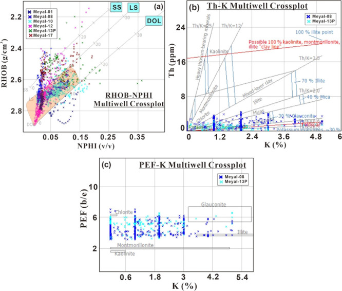
Cross-plot analysis for lithology identification. (a) NPHI vs RHOB multiwell cross-plot for all wells showing that limestone is the dominant lithology, having high RHOB and low NPHI values, which is highlighted by the orange-colored box. SS: sandstone; LS: limestone; DOL: dolomite. (b) Th vs K multiwell cross-plot revealing a variety of clay minerals within the targeted depths for M-08 and M-13P wells. (c) The PEF vs K cross-plot to confirm numerous clay minerals within the targeted depths of the reservoir for M-08 and M-13P wells.
4.3. Distinction of Oil and Water Zones by the Pickett Plot Technique
The Pickett plot depicts three types of areas in the reservoir, i.e., a water zone, an oil-water zone, and a classic oil zone. It is obvious that most of the plot shows the points between the first and second water saturation lines showing 25% Sw, which depicts the classic representation of an oil zone. There are very few points that lie below the 50% Sw line, which denote the water-bearing or oil–water zones. The results show that wells M-01 and M-17 (Figure 14a,f) have good oil-bearing zones as compared with other wells. Wells M-08, M-10, M-12, and M-13P (Figure 14b–e) show that the reservoir consists of oil zones along with oil–water and water zones. Overall, the results show that the reservoir within the MOF lies within the oil-bearing zones.
Figure 14.

Pickett plots for all studied wells, (a) M-01, (b) M-08, (c) M-10, (d) M-12, (e) M-13P, and (f) M-17, showing the distribution of dominant oil-bearing, oil–water, and water-bearing zones in the targeted depths of the reservoir region.
4.4. Lithofacies Classification Using SOM
An unsupervised learning model SOM was used to make the interpretation simpler and accurate. The logs used as input data curves for all studied wells to distribute the reservoir facies and create lithological sections are GR, RHOB, NPHI, and DT. Four input curves are used so that each node in the map can store its weighting for these four curves. To visually display the weightings on the map, a colored bar graph is shown (Figure 15a). SOM results after the calibration yield three main lithofacies with a color coding of green, gray, and pink. Each input point has a lattice connection to a point in the feature space, which ensures the safety of the neighborhood relationship between points. Three basic types of lithofacies were found in the area by running the software on the well-log data. The reservoir interval facies illustrate a slight variation in the lithological compositions.
Figure 15.

SOM results for lithofacies identification. Training of the SOM and curve distribution in all studied wells (a) before calibration and (b) after calibration. SOM results after calibration correspond to the three clusters of all studied wells. The green color denotes oil-bearing limestone facies, the gray color shows shaly sand, and the pink color shows the dolomite facies.
For the identification of the lithological profile of the interpreted wells, the specific color code’s distribution style is defined as a horizontal and vertical distribution feature. Facies in the reservoir region demonstrate slight variations in lithological components. Different color codes distinguish between limestone, shaly sand, and dolomite lithofacies. The facies with green color indicate pure limestone, whereas facies with color codings of gray and pink indicate shaly sand and dolomite, respectively (Figure 15b). The SOM model also showed the scale and potential of hydrocarbon variability, which has previously been acknowledged. A low proportion of clay in limestone indicates the presence of oil-bearing lithofacies. In contrast, the shaly sandstone and dolomite facies represent the non-oil-bearing lithofacies. The results of SOM are reliable to interpret and classify the lithofacies.
4.5. Comprehensive Interpretation of Multiminerals and Reservoir Zones Using Quanti-Elan Modeling
Quanti Elan is a probabilistic and multicomponent statistic modeling method. Interpretation results using the Quanti Elan module in all studied wells of MOF are elaborated in Figures 16–21. The track configuration is defined as follows: the 1st track displays the depth of the log in meters; the 2nd track consists of SP (mV), CALI (in), and GR (API) logs; resistivity (LLD, LLS, or MSFL depending on the availability of the logs in each well) (ohm/m–1) logs are shown in the 3rd track; the 4th track contains NPHI (v/v), RHOB (g/cm3), and DT (us/ft) logs; the 5th track shows the effective porosity (PHIE), water saturation (Sw), and the Coates method permeability (PERM) (mD); and the multiminerals, bound water, moved water, and moved hydrocarbon results are shown in the last track. In the multimineral results of Quanti Elan, dark gray represents illite clay mineral, the light-blue box indicates oil-bearing limestone, dark purple represents dolomite, orange indicates bound water, light green represents oil saturation, blue shows moved water, red shows moved hydrocarbons, and cyan shows water. The list of inputs used in the Quanti Elan model is shown in Table 2. The components in this case are limited to illite, limestone, dolomite, water saturation, and oil saturation. The number of components solved did not exceed the cumulative number of equations used. The dynamic analysis list used is presented in Table 3.
Figure 16.

Elan results for well M-01 display three reservoir zones with oil saturation. Track 1: depth; track 2: SP (mV), CALI (in), and GR (API) logs; track 3: resistivity (LLD, LLS, MSFL) (ohm/m–1) logs; track 4: NPHI (v/v), RHOB (g/cm3), and DT (us/ft) logs; track 5: PHIE, Sw, and the Coates method permeability (PERM) (mD); and track 6: multiminerals, bound water, moved water, and moved hydrocarbon. Zones A, B, and C are the possible reservoir zones, whereas the other highlighted zones are nonreservoir zones.
Figure 21.

Elan results for well M-17 display three reservoir zones with oil saturation. Track 1: depth; track 2: SP (mV), CALI (in), and GR (API) logs; track 3: resistivity (LLD, MSFL) (ohm/m–1) logs; track 4: NPHI (v/v), RHOB (g/cm3), and DT (us/ft) logs; track 5: PHIE, Sw, and the Coates method permeability (PERM) (mD); and track 6: multiminerals, bound water, moved water, and moved hydrocarbon. Zones A, B, and C are the possible reservoir zones, whereas the other highlighted zones are nonreservoir zones.
Table 2. List of Inputs Used in the Quanti Elan Model.
| family | uncertainties | uncertainty type | input weight | unflushed factor | equation type | type tool | constants | activate | |
|---|---|---|---|---|---|---|---|---|---|
| 1 | bulk density | 0.027 | absolute | 1 | 0 | linear | RHOB | yes | |
| 2 | neutron porosity | 0.015 | absolute | 1 | 0 | linear | NPHI | NPHI | yes |
| 3 | formation resistivity | 0.05 | relative | 1 | 1 | linear | yes | ||
| 4 | flushed zone resistivity | 0.05 | relative | 1 | 0 | linear | yes | ||
| 5 | compressional Slowness | 2.25 | absolute | 0.075 | 0 | linear | DT | yes | |
| 6 | porosity | 0.015 | absolute | 0.5 | 0 | linear | porosity | yes | |
| 7 | UI_GR | 1 | absolute | 1 | 0 | linear | yes |
Table 3. List of Component Specifications Used in the Quanti Elan Model.
| component specifications | |||||||
|---|---|---|---|---|---|---|---|
| illite | calcite | dolomite | XWater | XOil | UWater | UOil | |
| activate | yes | yes | yes | yes | yes | yes | yes |
| bulk density (g/cm3) | 2.79 | 2.71 | 2.87 | 1.209 | 0.7 | 1.209 | 0.7 |
| neutron porosity (v/v) | 1 | 0 | 0.004203 | 1 | 0.95 | 1 | 0.95 |
| compressional slowness (us/ft) | 90 | 47.5 | 43.5 | 189 | 210 | 189 | 210 |
| porosity (v/v) | 0 | 0 | 0 | 1 | 1 | 1 | 1 |
| UI_GR | –9999 | –9999 | –9999 | –9999 | –9999 | –9999 | –9999 |
| permittivity | 5.8 | 8.5 | 6.8 | 47.65 | 2.2 | 47.65 | 2.2 |
| conductivity (ohm/m) | 0 | 0 | 0 | 24.39 | 0 | 24.39 | 0 |
| min volume | 0 | 0 | 0 | 0 | 0 | 0 | 0 |
| max volume | 1 | 1 | 1 | 1 | 1 | 1 | 1 |
| Mx Type | shale | matrix | matrix | Xfluid | Xfluid | Ufluid | Ufluid |
| salinity (kppm) | 0 | 0 | 0 | 230 | 0 | 230 | 0 |
| PrmFac | –5.5 | –2 | 0 | –9999 | –9999 | –9999 | –9999 |
| Msa | 101 | 4 | 2 | –9999 | –9999 | –9999 | –9999 |
Figure 17.

Elan results for well M-08 display a thick reservoir zone with oil saturation. (Figure 16) Elan results for well M-01 display three reservoir zones with oil saturation. Track 1: depth; track 2: SP (mV), CALI (in), and GR (API) logs; track 3: resistivity (LLD, LLS, MSFL) (ohm/m–1) logs; track 4: NPHI (v/v), RHOB (g/cm3), and DT (us/ft) logs; track 5: PHIE, Sw, and the Coates method permeability (PERM) (mD); and track 6: multiminerals, bound water, moved water, and moved hydrocarbon. Zones A and B are the possible reservoir zones, whereas the other highlighted zones are nonreservoir zones.
Figure 18.

Elan results for well M-10 display three reservoir zones with oil saturation. Track 1: depth; track 2: SP (mV), CALI (in), and GR (API) logs; track 3: resistivity (LLD, LLS, MSFL) (ohm/m–1) logs; track 4: NPHI (v/v), RHOB (g/cm3), and DT (us/ft) logs; track 5: PHIE, Sw, and the Coates method permeability (PERM) (mD); and track 6: multiminerals, bound water, moved water, and moved hydrocarbon. Zones A, B, and C are the possible reservoir zones, whereas the other highlighted zones are nonreservoir zones.
Figure 19.

Elan results for well M-12 display three reservoir zones with oil saturation. Track 1: depth; track 2: SP (mV), CALI (in), and GR (API) logs; track 3: resistivity (LLD, MSFL) (ohm/m–1) logs; track 4: NPHI (v/v), RHOB (g/cm3), and DT (us/ft) logs; track 5: PHIE, Sw, and the Coates method permeability (PERM) (mD); and track 6: multiminerals, bound water, moved water, and moved hydrocarbon. Zones A, B, and C are the possible reservoir zones, whereas the other highlighted zones are nonreservoir zones.
Figure 20.

Elan results for well M-13P display four reservoir zones with oil saturation. Track 1: depth; track 2: SP (mV), CALI (in), and GR (API) logs; track 3: resistivity (LLD, MSFL) (ohm/m–1) logs; track 4: NPHI (v/v), RHOB (g/cm3), and DT (us/ft) logs; track 5: PHIE, Sw, and the Coates method permeability (PERM) (mD); and track 6: multiminerals, bound water, moved water, and moved hydrocarbon. Zones A, B, C, and D are the possible reservoir zones, whereas the other highlighted zones are nonreservoir zones.
A total of 17 reservoir zones in all study wells (M-01, M-08, M-10, M-12, M-13P, and M-17) were marked through petrophysical parameter evaluation having an oil detection zone at a depth ranging from 3700 to 4150 m. The results of Quanti Elan show almost the same results regarding the possible oil-bearing reservoir zones. Well M-01 contains two zones, whereas wells M-10, M-12, and M-17 contain three reservoir zones. Well M-13P contains four zones. However, well M-08 shows two reservoir zones containing oil. Zone C in the petrophysical analysis does not contain oil. Results of Quanti Elan show the presence of moved hydrocarbon below the Chorgali bottom formation. The presence of pores within the carbonates plays a major role in the migration of hydrocarbons within the MOF.55 The evidence of migration of hydrocarbons and dolomite facies below the Chorgali bottom formation makes the region unsuitable for containing oil. However, overall results are in agreement with pay thickness zones marked in the petrophysical analysis.
The variations in the reservoir depths in these wells indicate structural variations that are related to the extensional regime of the study area. The rift mechanism creates horse and graben structures within the region. The mean porosity ranges from 7.44 to 18.07%, which indicates a reasonable reservoir quality. The PERM values vary from 1.33 to 201.84 mD. The Indonesian model gives a pessimistic value of water saturation of the virgin zone, with an average value of 40%, compared with 50% as determined by Archie′s method. The maximum oil saturation can reach up to 69%, whereas the average oil saturation of the reservoir is approximately 51%. The results of Quanti Elan modeling are reliable and support the results of the petrophysical analysis, which also suggests the same depths of reservoir zones. In addition, multiminerals identified from Quanti Elan are the same as those determined from the cross-plot, Pickett plot, and SOM analysis. All of the petrophysical parameters along with the zones are shown in Table 4.
Table 4. Demarcated Reservoir Zones at Targeted Depths in All Studied Wells Using Quanti Elan Modeling.
| well names | Zonation | top (m) | base (m) | thickness (m) | PHIE (%) | Vsh (%) | Sw (%) | So (%) |
|---|---|---|---|---|---|---|---|---|
| Meyal-01 | Zone A | 3740 | 3765 | 15 | 16.2 | 10.8 | 38.5 | 61.4 |
| Zone B | 3773 | 3788 | 15 | 8.1 | 11.7 | 56.3 | 43.6 | |
| Meyal-08 | Zone A | 3700 | 3717 | 17 | 12.8 | 10.1 | 46.6 | 53.4 |
| Zone B | 3735 | 3746 | 11 | 9.8 | 12.1 | 50.7 | 49.3 | |
| Meyal-10 | Zone A | 3843 | 3855 | 12 | 10.5 | 12 | 41.2 | 58.8 |
| Zone B | 3862 | 3870 | 8 | 11.3 | 14.2 | 41 | 59 | |
| Zone C | 3888 | 3925 | 37 | 9.3 | 11.9 | 34.8 | 65.2 | |
| Meyal-12 | Zone A | 3707 | 3714 | 7 | 17.9 | 12.8 | 33.1 | 66.9 |
| Zone B | 3718 | 3724 | 6 | 16.8 | 13.9 | 50.1 | 49.9 | |
| Zone C | 3734 | 3741 | 7 | 16.3 | 12.7 | 40.4 | 59.8 | |
| Meyal-13P | Zone A | 4118 | 4121 | 3 | 18.9 | 11.6 | 31.4 | 68.6 |
| Zone B | 4126.5 | 4128.5 | 2 | 18.8 | 13.1 | 33.2 | 66.8 | |
| Zone C | 4133 | 4137 | 4 | 17.9 | 12.4 | 41.7 | 58.3 | |
| Zone D | 4146 | 4147 | 1 | 16.2 | 10.9 | 48.8 | 51.2 | |
| Meyal-17 | Zone A | 4106 | 4108 | 2 | 13.3 | 14.7 | 32.8 | 67.2 |
| Zone B | 4109 | 4110 | 1 | 11.2 | 14.8 | 46.8 | 53.2 | |
| Zone C | 4115.5 | 4116.5 | 1 | 11.1 | 15.7 | 55.4 | 44.6 |
4.6. Lateral Variation of Reservoir Parameters for the Evaluation of Favorable Oil Zones
The isopach maps of shale content (Vsh %), water saturation (Sw %), effective porosity (PHIE %), and hydrocarbon spatial distribution (HC %) of the reservoir in the research area were generated by Golden Surfer V8. The most important aspect to assess reservoir distribution is the lateral distribution of Vsh in the research area. Results show a high-scale shale content in the northwestern and southwestern regions of the research area, i.e., toward the M-08 well, whereas the Vsh values are medium toward the eastern region. However, the Vsh values are least at the middle region of the research area toward the M-12 and M-13P wells (Figure 22a). Northwest and southwest areas toward well M-08 show maximum Sw values, and toward wells M-01 and M-17, relatively medium values were determined. However, the middle region at wells M-12 and M-13P shows low values of Sw (Figure 22b).
Figure 22.

Lateral distribution maps: (a) average Vsh, (b) average Sw, (c) average PHIE, and (d) average HC.
The PHIE map also reveals that the porosity values decrease in the northwestern and southwestern parts of the research area but increase in the middle part toward M-12 and M-13P wells. PHIE increases along the direction in which the Vsh decreases and Sw decreases (Figure 22c). The oil saturation distribution map of the reservoir area reveals that higher concentrations can be seen in the central part of the research area, i.e., at wells M-12 and M-13P. A decrease in the concentration values was noticed in the overall western portion of the research area. The hydrocarbon saturation map shows that the concentration increases toward the southeastern portion of the research area, i.e., at well M-10 (Figure 22d). Therefore, we proposed that the most favorable and desirable regions for oil saturation are the central and southeastern portions of the research area. Wells M-10, M-12, and M-13P lie at the most favorable zones, whereas wells M-01 and M-17 lie in the medium HC potential zone, and well M-08 lies in the low-porosity zone and can be regarded as a tight oil reservoir.
4.7. Implications of the Reservoir Parameter Distribution and the Role of Reservoir Exploration and Development
The purpose of this study was to present a clear and distinct understanding of the reservoir parameter distribution to investigate the reservoir exploration and development of the MOF. The gist of the results suggested that Chorgali has more potential oil-bearing reservoir zones as compared with the Sakesar Formation. Wells M-01, M-08, M-10, and M-12 show multiple reservoir zones within the Chorgali Formation. Barring the reservoir in Chorgali–Sakesar Formations, regions near the Lockhart Formation also have the potential for containing oil. Many diagenetic processes, including micritization, dolomitization, cementation, neomorphism, dissolution, compaction (mechanical and chemical, i.e., stylolitization), and fracturing, have altered the Chorgali Formation.55 Diagenetic processes play an important role in altering the quality of the reservoir and affect the stratigraphic–structural play significantly.23,87−89 In the case of the Chorgali Formation within the MOF, the diagenetic processes enhancing the reservoir quality include dolomitization, dissolution, and fracturing. However, micritization, cementation, neomorphism, and compaction played major roles in reducing the reservoir properties. In addition, the kind of porosity contributes not only to the storage and migration of hydrocarbons via pores but also to the comprehension and interpretation of the seismic characteristics of carbonates.55 The migration of hydrocarbons through the pores is evident through the Quanti Elan interpretation of the M-08 well. In addition to the Chorgali Formation, the Sakesar Formation also shows the same characteristics. The Sakesar Limestone and the Chorgali Formation both have a thickness of around 183 m (600 feet) and comprise alternating layers of limestone and shale. This indicates the presence of compartmentalized reservoirs throughout the Eocene sequence.1 Therefore, the Eocene deposits play a significant role in the reservoir exploration and development of the MOF. However, in addition to the Eocene (Chorgali–Sakesar) deposits, the Paleocene deposits near the Lockhart Formation also contain oil-bearing zones, which are quite significant and evident within the M-13P. According to a recent study, the Lockhart Limestone exhibits a variety of diagenetic phenomena. Some of these features include mechanical and chemical compaction, deep burial water pressure, pressure solution, and tectonics-related fracture.90 In the previous study, it was suggested that the Lockhart Formation contained oil and that it flowed at a rate of 659 barrels of oil per day (BOPD).2 Therefore, the vast hydrocarbon potential of the Paleocene carbonates near the Lockhart Formation should also be focused on. The Eocene Formations in the Meyal region in the Potwar Basin in Pakistan have strong reservoir characteristics and emerge in seismic sections with advantageous structural traps that are associated both with pop-up anticlines and thrusts [1]. Therefore, we propose that along with Eocene carbonate deposits, the Paleocence deposits should not be neglected. For further evaluation of the hydrocarbon potential, seismic data along with cores should be thoroughly investigated. Furthermore, the marked reservoir zones in our study should be adequately evaluated with further quantitative and qualitative analyses to enhance the possibilities of new horizons in terms of oil production and development within the Potwar Basin of Pakistan.
5. Conclusions
The main conclusions are as follows;
-
(1)
A total of 17 reservoir pay zones were identified within the six studied wells of the targeted Sakesar and Chorgali Formations. These 17 regions lie in the 3700–4150 m region. The difference in reservoir depths in different wells suggests the presence of structural variations that are associated with extensional regimes of the study area.
-
(2)
The lithology was analyzed with NPHI-RHOB, K-Th, and PEF-K cross-plots, which show that limestone is the dominant lithology, whereas clay minerals consist mainly of illite, glauconite, and chlorite.
-
(3)
The results of the Pickett plots showed that the targeted depths of the reservoir were mainly composed of oil-bearing limestone zones having a water saturation of less than 50%. However, oil–water and water zones have a lower log response than the oil-bearing zones.
-
(4)
Likewise, the advanced technique of unsupervised machine learning of SOM was used for lithofacies classification, which yielded three main facies in the reservoir area, with limestone regarded as the main lithofacies. The other lithofacies are shaly sand and dolomite.
-
(5)
The results of the novel Quanti Elan modeling revealed that there is an oil detection zone at a depth ranging from 3700 m to 4100 m. Eighteen reservoir zones within wells (M-01, M-08, M-10, M-12, M-13P, M-16, and M-17) were depicted with petrophysical parameter evaluation. The variations between the reservoir depths suggest the heterogeneous nature of the area. The maximum oil saturation can reach up to 69%, whereas the average oil saturation of the reservoir is approximately 51%. The mean PHIE ranges from 7.44 to 18.07%, which indicates a reasonable reservoir quality, and the permeability varies from 1.33 to 201.84 mD. Several porous zones are present in the reservoir, but some of them lack sufficient permeability to produce commercial hydrocarbons. Perhaps this should be due to the availability of shale content in the reservoir area, which can adversely affect the reservoir quality.
-
(6)
The lateral mapping of the petrophysical parameters suggested that the most favorable regions for oil saturation lie toward the central portion and southeastern regions of the research area. The most favorable zones are located at wells M-10, M-12, and M-13P, respectively. However, wells M-01 and M-17 are both located in a zone with a medium HC potential, whereas well M-08 is located in a zone with low porosity and is considered to be a tight oil reservoir.
Acknowledgments
The authors thank the Directorate General of Petroleum Concessions (DGPC), Pakistan, for the release of well data. This study was supported by the National Natural Science Foundation of China (No. 42062015) and the Natural Science Foundation of Guangxi (No. 2018AD19204). The authors also extend their gratitude to Yunnan Provincial Government Leading Scientist Program, No. 2015HA024.
Author Present Address
○ Institute of Deep-Sea Science and Engineering, Chinese Academy of Sciences, Sanya 572000, China
Author Contributions
¶ J.A. and U.A. contributed equally to this work. First authorship is shared between J.A. and U.A.
The authors declare no competing financial interest.
References
- Riaz M.; Pimentel N.; Ghazi S.; Zafar T.; Alam A.; Ariser S. Lithostratigraphic analysis of the Eocene reservoir units of Meyal area, Potwar Basin, Pakistan. Himalayan Geol. 2018, 39, 161–170. [Google Scholar]
- Hasany S. T.; Saleem U.. An integrated subsurface geological and engineering study of Meyal Field, Potwar Plateau, Pakistan Search Discovery Article 20151 2012, pp 1–41.
- Ehsan M.; Gu H.; Akhtar M. M.; Abbasi S. S.; Ullah Z. Identification of hydrocarbon potential of Talhar shale: Member of lower Goru Formation using well logs derived parameters, southern lower Indus basin, Pakistan. J. Earth Sci. 2018, 29, 587–593. 10.1007/s12583-016-0910-2. [DOI] [Google Scholar]
- Li Y.; Zhou L.; Li D.; Zhang S.; Tian F.; Xie Z.; Liu B. Shale brittleness index based on the energy evolution theory and evaluation with logging data: a case study of the Guandong block. Acs Omega 2020, 5, 13164–13175. 10.1021/acsomega.0c01140. [DOI] [PMC free article] [PubMed] [Google Scholar]
- Ehsan M.; Gu H.; Ahmad Z.; Akhtar M. M.; Abbasi S. S. A modified approach for volumetric evaluation of shaly sand formations from conventional well logs: A case study from the talhar shale, Pakistan. Arabian J. Sci. Eng. 2019, 44, 417–428. 10.1007/s13369-018-3476-8. [DOI] [Google Scholar]
- Liu Z.; Chen D.; Zhang J.; Lv X.; Dang W.; Liu Y.; Liao W.; Li J.; Wang Z.; Wang F. Combining Isotopic Geochemical Data and Logging Data to Predict the Range of the Total Gas Content in Shale: A Case Study from the Wufeng and Longmaxi Shales in the Middle Yangtze Area, South China. Energy Fuels 2019, 33, 10487–10498. 10.1021/acs.energyfuels.9b01879. [DOI] [Google Scholar]
- Mahmood M. F.; Ahmad Z.; Ehsan M. Total organic carbon content and total porosity estimation in unconventional resource play using integrated approach through seismic inversion and well logs analysis within the Talhar Shale, Pakistan. J. Nat. Gas Sci. Eng. 2018, 52, 13–24. 10.1016/j.jngse.2018.01.016. [DOI] [Google Scholar]
- Radwan A. E. Modeling the depositional environment of the sandstone reservoir in the Middle Miocene Sidri Member, Badri Field, Gulf of Suez Basin, Egypt: Integration of gamma-ray log patterns and petrographic characteristics of lithology. Nat. Resour. Res. 2021, 30, 431–449. 10.1007/s11053-020-09757-6. [DOI] [Google Scholar]
- Ibrahim A. F.; Elkatatny S.; Al Ramadan M. Prediction of Water Saturation in Tight Gas Sandstone Formation Using Artificial Intelligence. ACS Omega 2022, 7, 215–222. 10.1021/acsomega.1c04416. [DOI] [PMC free article] [PubMed] [Google Scholar]
- Quijada M. F.; Steward R.. Petrophysical Analysis of Well Logs from Manitou Lake, CREWERS Research Report; Saskatchewan Pulse Growers, 2007.
- Radwan A. E.; Abudeif A.; Attia M. Investigative petrophysical fingerprint technique using conventional and synthetic logs in siliciclastic reservoirs: A case study, Gulf of Suez basin, Egypt. J. Afr. Earth Sci. 2020, 167, 103868 10.1016/j.jafrearsci.2020.103868. [DOI] [Google Scholar]
- Tariq Z.; Mahmoud M.; Abouelresh M.; Abdulraheem A. Data-driven approaches to predict thermal maturity indices of organic matter using artificial neural networks. ACS Omega 2020, 5, 26169–26181. 10.1021/acsomega.0c03751. [DOI] [PMC free article] [PubMed] [Google Scholar]
- Asquith G. B.; Gibson C. R.. Basic Well Log Analysis for Geologists; American Association of Petroleum Geologists: Tulsa, 1982; Vol. 3. [Google Scholar]
- Mangi H. N.; Detian Y.; Hameed N.; Ashraf U.; Rajper R. H. Pore structure characteristics and fractal dimension analysis of low rank coal in the Lower Indus Basin, SE Pakistan. J. Nat. Gas Sci. Eng. 2020, 77, 103231 10.1016/j.jngse.2020.103231. [DOI] [Google Scholar]
- Vo Thanh H.; Sugai Y.; Sasaki K. Impact of a new geological modelling method on the enhancement of the CO2 storage assessment of E sequence of Nam Vang field, offshore Vietnam. Energy Sources, Part A 2020, 42, 1499–1512. 10.1080/15567036.2019.1604865. [DOI] [Google Scholar]
- Yasin Q.; Sohail G. M.; Ding Y.; Ismail A.; Du Q. Estimation of petrophysical parameters from seismic inversion by combining particle swarm optimization and multilayer linear calculator. Nat. Resour. Res. 2020, 29, 3291–3317. 10.1007/s11053-020-09641-3. [DOI] [Google Scholar]
- Alao P. A.; Ata A.; Nwoke C. Subsurface and petrophysical studies of shaly-sand reservoir targets in Apete field, Niger Delta. ISRN Geophys. 2013, 2013, 1–11. 10.1155/2013/102450. [DOI] [Google Scholar]
- Ali M.; Ma H.; Pan H.; Ashraf U.; Jiang R. Building a rock physics model for the formation evaluation of the Lower Goru sand reservoir of the Southern Indus Basin in Pakistan. J. Pet. Sci. Eng. 2020, 194, 107461 10.1016/j.petrol.2020.107461. [DOI] [Google Scholar]
- Ali N.; Chen J.; Fu X.; Hussain W.; Ali M.; Hussain M.; Anees A.; Rashid M.; Thanh H. V. Prediction of Cretaceous reservoir zone through petrophysical modeling: Insights from Kadanwari gas field, Middle Indus Basin. Geosyst. Geoenviron. 2022, 1, 100058 10.1016/j.geogeo.2022.100058. [DOI] [Google Scholar]
- Storvoll V.; Bjørlykke K.; Karlsen D.; Saigal G. Porosity preservation in reservoir sandstones due to grain-coating illite: a study of the Jurassic Garn Formation from the Kristin and Lavrans fields, offshore Mid-Norway. Mar. Pet. Geol. 2002, 19, 767–781. 10.1016/S0264-8172(02)00035-1. [DOI] [Google Scholar]
- Vo Thanh H.; Sugai Y.; Nguele R.; Sasaki K. In A New Petrophysical Modeling Workflow for Fractured Granite Basement Reservoir in Cuu Long Basin, Offshore Vietnam, Proceedings of the 81st EAGE Conference and Exhibition 2019; EarthDoc, 2019; pp 1–5, 10.3997/2214-4609.201900706. [DOI]
- Vo Thanh H.; Sugai Y.; Nguele R.; Sasaki K. Integrated workflow in 3D geological model construction for evaluation of CO2 storage capacity of a fractured basement reservoir in Cuu Long Basin, Vietnam. Int. J. Greenhouse Gas Control 2019, 90, 102826 10.1016/j.ijggc.2019.102826. [DOI] [Google Scholar]
- Dar Q. U.; Pu R.; Baiyegunhi C.; Shabeer G.; Ali R. I.; Ashraf U.; Sajid Z.; Mehmood M. The impact of diagenesis on the reservoir quality of the early Cretaceous Lower Goru sandstones in the Lower Indus Basin, Pakistan. J. Pet. Explor. Prod. Technol. 2022, 12, 1437–1452. 10.1007/s13202-021-01415-8. [DOI] [Google Scholar]
- Kassab M. A.; Abbas A.E.-S.; Teama M. A.; Khalifa M. A. Prospect evaluation and hydrocarbon potential assessment: the Lower Eocene Facha non-clastic reservoirs, Hakim Oil Field (NC74A), Sirte basin, Libya–a case study. J. Pet. Explor. Prod. Technol. 2020, 10, 351–362. 10.1007/s13202-019-00773-8. [DOI] [Google Scholar]
- Singh P. K.; Singh V.; Rajak P.; Mathur N. A study on assessment of hydrocarbon potential of the lignite deposits of Saurashtra basin, Gujarat (Western India). Int. J. Coal Sci. Technol. 2017, 4, 310–321. 10.1007/s40789-017-0186-x. [DOI] [Google Scholar]
- Zhang B.; Tong Y.; Du J.; Hussain S.; Jiang Z.; Ali S.; Ali I.; Khan M.; Khan U. Three-dimensional structural modeling (3D SM) and joint geophysical characterization (JGC) of hydrocarbon reservoir. Minerals 2022, 12, 363 10.3390/min12030363. [DOI] [Google Scholar]
- Anees A.; Zhang H.; Ashraf U.; Wang R.; Liu K.; Abbas A.; Ullah Z.; Zhang X.; Duan L.; Liu F.; et al. Sedimentary facies controls for reservoir quality prediction of lower shihezi member-1 of the Hangjinqi area, Ordos Basin. Minerals 2022, 12, 126 10.3390/min12020126. [DOI] [Google Scholar]
- Anees A.; Zhang H.; Ashraf U.; Wang R.; Liu K.; Mangi H.; Jiang R.; Zhang X.; Liu Q.; Tan S.; Shi W. Identification of Favorable Zones of Gas Accumulation Via Fault Distribution and Sedimentary Facies: Insights from Hangjinqi Area, Northern Ordos Basin. Front. Earth Sci. 2022, 9, 822670 10.3389/feart.2021.822670. [DOI] [Google Scholar]
- Ashraf U.; Zhu P.; Yasin Q.; Anees A.; Imraz M.; Mangi H. N.; Shakeel S. Classification of reservoir facies using well log and 3D seismic attributes for prospect evaluation and field development: A case study of Sawan gas field, Pakistan. J. Pet. Sci. Eng. 2019, 175, 338–351. 10.1016/j.petrol.2018.12.060. [DOI] [Google Scholar]
- Khan U.; Zhang B.; Du J.; Jiang Z. 3D structural modeling integrated with seismic attribute and petrophysical evaluation for hydrocarbon prospecting at the Dhulian Oilfield, Pakistan. Front. Earth Sci. 2021, 15, 649–675. 10.1007/s11707-021-0881-1. [DOI] [Google Scholar]
- Abdel-Fattah M. I.; Mahdi A. Q.; Theyab M. A.; Pigott J. D.; Abd-Allah Z. M.; Radwan A. E. Lithofacies classification and sequence stratigraphic description as a guide for the prediction and distribution of carbonate reservoir quality: a case study of the Upper Cretaceous Khasib Formation (East Baghdad oilfield, central Iraq). J. Pet. Sci. Eng. 2022, 209, 109835 10.1016/j.petrol.2021.109835. [DOI] [Google Scholar]
- Aplin G. F.; Dawans J.-M.L.; Sapru A. K.. New Insights from Old Data: Identification of Rock Types and Permeability Prediction Within a Heterogeneous Carbonate Reservoir Using Diplog and Openhole Log Data, Proceedings of the Abu Dhabi International Petroleum Exhibition and Conference; OnePetro, 2002 10.2118/78501-MS. [DOI]
- Boutaleb K.; Baouche R.; Sadaoui M.; Radwan A. E. Sedimentological, petrophysical, and geochemical controls on deep marine unconventional tight limestone and dolostone reservoir: Insights from the Cenomanian/Turonian oceanic anoxic event 2 organic-rich sediments, Southeast Constantine Basin, Algeria. Sediment. Geol. 2022, 429, 106072 10.1016/j.sedgeo.2021.106072. [DOI] [Google Scholar]
- Jiang R.; Zhao L.; Xu A.; Ashraf U.; Yin J.; Song H.; Su N.; Du B.; Anees A. Sweet spots prediction through fracture genesis using multi-scale geological and geophysical data in the karst reservoirs of Cambrian Longwangmiao Carbonate Formation, Moxi-Gaoshiti area in Sichuan Basin, South China. J. Pet. Explor. Prod. Technol. 2022, 12, 1313–1328. 10.1007/s13202-021-01390-0. [DOI] [Google Scholar]
- Radwan A. E.; Trippetta F.; Kassem A. A.; Kania M. Multi-scale characterization of unconventional tight carbonate reservoir: Insights from October oil filed, Gulf of Suez rift basin, Egypt. J. Pet. Sci. Eng. 2021, 197, 107968 10.1016/j.petrol.2020.107968. [DOI] [Google Scholar]
- Ali M.; Jiang R.; Ma H.; Pan H.; Abbas K.; Ashraf U.; Ullah J. Machine learning-A novel approach of well logs similarity based on synchronization measures to predict shear sonic logs. J. Pet. Sci. Eng. 2021, 203, 108602 10.1016/j.petrol.2021.108602. [DOI] [Google Scholar]
- Al-Mudhafar W. J. Integrating well log interpretations for lithofacies classification and permeability modeling through advanced machine learning algorithms. J. Pet. Explor. Prod. Technol. 2017, 7, 1023–1033. 10.1007/s13202-017-0360-0. [DOI] [Google Scholar]
- Ashraf U.; Zhang H.; Anees A.; Mangi H. N.; Ali M.; Zhang X.; Imraz M.; Abbasi S. S.; Abbas A.; Ullah Z.; et al. A core logging, machine learning and geostatistical modeling interactive approach for subsurface imaging of lenticular geobodies in a clastic depositional system, SE Pakistan. Nat. Resour. Res. 2021, 30, 2807–2830. 10.1007/s11053-021-09849-x. [DOI] [Google Scholar]
- Ashraf U.; Zhang H.; Anees A.; Nasir Mangi H.; Ali M.; Ullah Z.; Zhang X. Application of unconventional seismic attributes and unsupervised machine learning for the identification of fault and fracture network. Appl. Sci. 2020, 10, 3864 10.3390/app10113864. [DOI] [Google Scholar]
- Ehsan M.; Gu H. An integrated approach for the identification of lithofacies and clay mineralogy through Neuro-Fuzzy, cross plot, and statistical analyses, from well log data. J. Earth Syst. Sci. 2020, 129, 1–13. 10.1007/s12040-020-1365-5. [DOI] [Google Scholar]
- Feng R. A Bayesian approach in machine learning for lithofacies classification and its uncertainty analysis. IEEE Geosci. Remote Sens. Lett. 2021, 18, 18–22. 10.1109/LGRS.2020.2968356. [DOI] [Google Scholar]
- Kim J. Lithofacies classification integrating conventional approaches and machine learning technique. J. Nat. Gas Sci. Eng. 2022, 100, 104500 10.1016/j.jngse.2022.104500. [DOI] [Google Scholar]
- Jafarizadeh F.; Rajabi M.; Tabasi S.; Seyedkamali R.; Davoodi S.; Ghorbani H.; Alvar M. A.; Radwan A. E.; Csaba M. Data driven models to predict pore pressure using drilling and petrophysical data. Energy Rep. 2022, 8, 6551–6562. 10.1016/j.egyr.2022.04.073. [DOI] [Google Scholar]
- Kamali M. Z.; Davoodi S.; Ghorbani H.; Wood D. A.; Mohamadian N.; Lajmorak S.; Rukavishnikov V. S.; Taherizade F.; Band S. S. Permeability prediction of heterogeneous carbonate gas condensate reservoirs applying group method of data handling. Mar. Pet. Geol. 2022, 139, 105597 10.1016/j.marpetgeo.2022.105597. [DOI] [Google Scholar]
- Rajabi M.; Hazbeh O.; Davoodi S.; Wood D. A.; Tehrani P. S.; Ghorbani H.; Mehrad M.; Mohamadian N.; Rukavishnikov V. S.; Radwan A. E. Predicting shear wave velocity from conventional well logs with deep and hybrid machine learning algorithms. J. Pet. Explor. Prod. Technol. 2022, 0, 1–24. 10.1007/s13202-022-01531-z. [DOI] [Google Scholar]
- Safaei-Farouji M.; Thanh H. V.; Dai Z.; Mehbodniya A.; Rahimi M.; Ashraf U.; Radwan A. E. Exploring the power of machine learning to predict carbon dioxide trapping efficiency in saline aquifers for carbon geological storage project. J. Cleaner Prod. 2022, 372, 133778 10.1016/j.jclepro.2022.133778. [DOI] [Google Scholar]
- Safaei-Farouji M.; Thanh H. V.; Dashtgoli D. S.; Yasin Q.; Radwan A. E.; Ashraf U.; Lee K.-K. Application of robust intelligent schemes for accurate modelling interfacial tension of CO2 brine systems: Implications for structural CO2 trapping. Fuel 2022, 319, 123821 10.1016/j.fuel.2022.123821. [DOI] [Google Scholar]
- Tabasi S.; Tehrani P. S.; Rajabi M.; Wood D. A.; Davoodi S.; Ghorbani H.; Mohamadian N.; Alvar M. A. Optimized machine learning models for natural fractures prediction using conventional well logs. Fuel 2022, 326, 124952 10.1016/j.fuel.2022.124952. [DOI] [Google Scholar]
- Zhang G.; Davoodi S.; Shamshirband S.; Ghorbani H.; Mosavi A.; Moslehpour M. A robust approach to pore pressure prediction applying petrophysical log data aided by machine learning techniques. Energy Rep. 2022, 8, 2233–2247. 10.1016/j.egyr.2022.01.012. [DOI] [Google Scholar]
- Verma S.; Bhattacharya S.; Chowdhury N.U.M.K.; Tian M. In A New Workflow for Multi-well Lithofacies Interpretation Integrating Joint Petrophysical Inversion, Unsupervised, and Supervised Machine Learning, Proceedings of the First International Meeting for Applied Geoscience & Energy; SEG Library, 2021; pp 2213–2217 10.1190/segam2021-3584118.1. [DOI]
- Chang H.-C.; Kopaska-Merkel D. C.; Chen H.-C. Identification of lithofacies using Kohonen self-organizing maps. Comput. Geosci. 2002, 28, 223–229. 10.1016/S0098-3004(01)00067-X. [DOI] [Google Scholar]
- Yu G.; Aguilera R. In Use of Pickett Plots for Evaluation of Shale Gas Formations, Proceedings of the SPE Annual Technical Conference and Exhibition; OnePetro, 2011, 10.2118/146948-MS. [DOI]
- Waszkiewicz S.; Alvarez R. B.; Jarzyna J. Results of the comprehensive interpretation of well logs in carbonate and siliciclastic rocks–similarities and differences in the case studies of selected formations. Geol., Geophys. Environ. 2019, 45, 163 10.7494/geol.2019.45.3.163. [DOI] [Google Scholar]
- Ashraf U.; Zhang H.; Anees A.; Ali M.; Zhang X.; Shakeel Abbasi S.; Nasir Mangi H. Controls on reservoir heterogeneity of a shallow-marine reservoir in Sawan Gas Field, SE Pakistan: Implications for reservoir quality prediction using acoustic impedance inversion. Water 2020, 12, 2972 10.3390/w12112972. [DOI] [Google Scholar]
- Awais M.; Hanif M.; Khan M. Y.; Jan I. U.; Ishaq M. Relating petrophysical parameters to petrographic interpretations in carbonates of the Chorgali Formation, Potwar Plateau, Pakistan. Carbonates Evaporites 2019, 34, 581–595. 10.1007/s13146-017-0414-x. [DOI] [Google Scholar]
- Awais M.; Ullah F.; Khan N.; Ghani M.; Siyar S. M.; Wadood B.; Mukhtiar A. Investigation of reservoir characteristics, depositional setting and T–R sequences of the Lockhart Limestone of Meyal Oil Field, Pakistan: a petrophysical approach. J. Pet. Explor. Prod. Technol. 2019, 9, 2511–2530. 10.1007/s13202-019-0730-x. [DOI] [Google Scholar]
- Kazmi A. H.; Jan M. Q.. Geology and Tectonics of Pakistan; Graphic Publishers, 1997. [Google Scholar]
- Sercombe W. J.; Pivnik D. A.; Wilson W. P.; Albertin M. L.; Beck R. A.; Stratton M. A. Wrench faulting in the northern Pakistan foreland. AAPG Bull. 1998, 82, 2003–2030. 10.1190/1.1436997. [DOI] [Google Scholar]
- Siddiqui S.; Elahi N.; Siddiqui A. In Ratana Field–A Case History: Case Histories of Eight Oil and Gas Fields in Pakistan, Proceedings of Pakistan petroleum convention; American Association of Petroleum Geologist Search and Discovery Article 90145, 1998.
- Anees A.; Zhong S. W.; Ashraf U.; Abbas A. Development of a computer program for zoeppritz energy partition equations and their various approximations to affirm presence of hydrocarbon in missakeswal area. Geoscience 2017, 7, 55–67. 10.3390/geosciences7030055. [DOI] [Google Scholar]
- Kadri I. B.Petroleum Geology of Pakistan; Pakistan Petroleum Limited, 1995. [Google Scholar]
- Khan A. A.; Ahmad S.; Khan M. I. Hydrocarbon Prospects of Karak anticline, NW Pakistan: Myths and Facts. Pak. J. Hydrocarbon Res. 2008, 18, 51–64. [Google Scholar]
- Ghazi S.; Ali A.; Hanif T.; Sharif S.; Arif S. J. Larger benthic foraminiferal assemblage from the Early Eocene Chor Gali Formation, Salt Range, Pakistan. Geol. Bull. Punjab Univ. 2010, 45, 83–91. [Google Scholar]
- Ghazi S.; Aziz T.; Khalid P.; Sahraeyan M. Petroleum play analysis of the Jurassic sequence, Meyal-field, Potwar basin, Pakistan. J. Geol. Soc. India 2014, 84, 727–738. 10.1007/s12594-014-0183-2. [DOI] [Google Scholar]
- Grana D.; Pirrone M.; Mukerji T. Quantitative log interpretation and uncertainty propagation of petrophysical properties and facies classification from rock-physics modeling and formation evaluation analysis. Geophysics 2012, 77, WA45–WA63. 10.1190/geo2011-0272.1. [DOI] [Google Scholar]
- Clark B. O.Patent and Trademark Office. US9, 217,323, 2015.
- Lai J.; Wang G.; Chai Y.; Ran Y. Prediction of diagenetic facies using well logs: Evidences from Upper Triassic Yanchang Formation Chang 8 sandstones in Jiyuan region, Ordos basin, China. Oil Gas Sci. Technol. 2016, 71, 34. 10.2516/ogst/2014060. [DOI] [Google Scholar]
- Hamada G. In An Integrated Approach to Determine Shale Volume and Hydrocarbon Potential in Shaly Sand in The Gulf Of Suez, Proceedings of the SCA International Symposium; OnePetro, 1996; pp 2093–2107.
- Stieber S. In Pulsed Neutron Capture Log Evaluation-Louisiana Gulf Coast, Proceedings of the Fall Meeting of the Society of Petroleum Engineers of AIME; OnePetro, 1970.
- Larionov V.Borehole Radiometry Nedra, Moscow, 1969; Vol. 127, p 813. [Google Scholar]
- Ullah J.; Luo M.; Ashraf U.; Pan H.; Anees A.; Li D.; Ali M.; Ali J. Evaluation of the geothermal parameters to decipher the thermal structure of the upper crust of the Longmenshan fault zone derived from borehole data. Geothermics 2022, 98, 102268 10.1016/j.geothermics.2021.102268. [DOI] [Google Scholar]
- Akhanda A.; Islam M.. Introduction to Petroleum Geology and Drilling Publication-cum-Information Office, Bangladesh, 1994; Vol. 78. [Google Scholar]
- Doveton J.Basics of oil and gas log analysis Kans. Geol. Surv. 1999; Vol. 510.
- Leveaux J.; Poupon A.. Evaluation of Water Saturation in Shaly Formations. In The Log Analyst; OnePetro, 1971, p 12.
- Widarsono B. Choice of water saturation model in log analysis and its implication to water saturation estimates–a further investigation. Sci. Contrib. Oil Gas 2012, 35, 99–107. 10.29017/SCOG.35.3.782. [DOI] [Google Scholar]
- Shang B. Z.; Hamman J. G.; Chen H.-L.; Caldwell D. H. In A Model to Correlate Permeability with Efficient Porosity and Irreducible Water Saturation, Proceedings of the SPE Annual Technical Conference and Exhibition; OnePetro, 2003.
- Coates G. R.; Dumanoir J. In A New Approach to Improved Log-Derived Permeability, Proceedings of the SPWLA 14th Annual Logging Symposium; OnePetro, 1973.
- Malaieri M.; Matoorian R.; Aguilera R. In A New Approach for Geomechanical Evaluations with Modified Pickett Plots, Proceedings of the SPE Latin American and Caribbean Petroleum Engineering Conference; OnePetro, 2020.
- Chudi O.; Simon R. In Petrophysical Characterization of Radioactive Sands-Integrating Well Logs and Core Information: A Case Study in the Niger Delta, Proceedings of the Nigeria Annual International Conference and Exhibition; OnePetro, 2012.
- Chang E.; Zung L. S.; ICIPEG . 3D Reservoir Characterization of Field Deta; Springer: Termit Basin, Niger, 2016; Vol. 2017, pp 323–335. [Google Scholar]
- Baban D. H.; Qadir F. M.; Mohammed A. R. Reservoir rock properties of the Upper Cretaceous Shiranish Formation in Taq Taq Oilfield, Iraqi Kurdistan Region. J. Zankoy Slemani 2020, 22, 363–388. 10.17656/jzs.10799. [DOI] [Google Scholar]
- Flores R. M.; Keighin C. W.. Petrology and Depositional Facies of Siliciclastic Rocks of the Middle Ordovician Simpson Group; US Government Printing Office: Mazur Well, Southeastern Anadarko Basin, Oklahoma, 1989. [Google Scholar]
- Mai-Cao L.; Le C. A Self-Organizing Map, Machine Learning Approach to Lithofacies Classification. Int. J. Simul.:Syst., Sci. Technol. 2018, 19, 16.1–16.6. 10.5013/IJSSST.a.19.03.16. [DOI] [Google Scholar]
- Murtagh F.; Hernández-Pajares M. The Kohonen self-organizing map method: an assessment. J. Classif. 1995, 12, 165–190. 10.1007/BF03040854. [DOI] [Google Scholar]
- Sharma M.; Singh K. H.; Pandit S.; Kumar A.; Soni A.. Petrophysical Modelling of Carbonate Reservoir from Bombay Offshore Basin. In Petro-physics and Rock Physics of Carbonate Reservoirs; Springer, 2020; pp 55–69. [Google Scholar]
- Tian Y.; Ayers W. B. In Barnett Shale (Mississippian), Fort Worth Basin, Texas: Regional Variations in Gas and Oil Production and Reservoir Properties, Proceedings of the Canadian Unconventional Resources and International Petroleum Conference; OnePetro, 2010.
- El-Gendy N. H.; Radwan A. E.; Waziry M. A.; Dodd T. J.; Barakat M. K. An integrated sedimentological, rock typing, image logs, and artificial neural networks analysis for reservoir quality assessment of the heterogeneous fluvial-deltaic Messinian Abu Madi reservoirs, Salma field, onshore East Nile Delta, Egypt. Mar. Pet. Geol. 2022, 145, 105910 10.1016/j.marpetgeo.2022.105910. [DOI] [Google Scholar]
- Nabawy B. S.; Abudeif A. M.; Masoud M. M.; Radwan A. E. An integrated workflow for petrophysical characterization, microfacies analysis, and diagenetic attributes of the Lower Jurassic type section in northeastern Africa margin: Implications for subsurface gas prospection. Mar. Pet. Geol. 2022, 140, 105678 10.1016/j.marpetgeo.2022.105678. [DOI] [Google Scholar]
- Radwan A. E.; Rohais S.; Chiarella D. Combined stratigraphic-structural play characterization in hydrocarbon exploration: a case study of Middle Miocene sandstones, Gulf of Suez basin, Egypt. J. Asian Earth Sci. 2021, 218, 104686 10.1016/j.jseaes.2021.104686. [DOI] [Google Scholar]
- Khattak Z.; Khan M. A.; Rahman Z.; Ishfaque M.; Yasir M. Microfacies and diagenetic analysis of Lockhart Limestone, Shah Alla Ditta area Islamabad, Pakistan. Pak. J. Geol. 2017, 1, 24–26. 10.26480/pjg.01.2017.24.26. [DOI] [Google Scholar]